QCWAVE - A MATHEMATICA QUANTUM COMPUTER SIMULATION UPDATE

Abstract

This Mathematica 7.0/8.0 package upgrades and extends the quantum computer simulation code called QDENSITY. Use of the density matrix was emphasized in QDENSITY, although that code was also applicable to a quantum state description. In the present version, the quantum state version is stressed and made amenable to future extensions to parallel computer simulations. The add-on QCWAVE extends QDENSITY in several ways. The first way is to describe the action of one, two and three- qubit quantum gates as a set of small ($2\times 2,4\times 4$ or $8\times 8$) matrices acting on the $2^{n_{q}}$ amplitudes for a system of $n_{q}$ qubits. This procedure was described in our parallel computer simulation QCMPI and is reviewed here. The advantage is that smaller storage demands are made, without loss of speed, and that the procedure can take advantage of message passing interface (MPI) techniques, which will hopefully be generally available in future Mathematica versions.

Another extension of QDENSITY provided here is a multiverse approach, as described in our QCMPI paper. This multiverse approach involves using the present slave-master parallel processing capabilities of Mathematica 7.0/8.0 to simulate errors and error correction. The basic idea is that parallel versions of QCWAVE run simultaneously with random errors introduced on some of the processors, with an ensemble average used to represent the real world situation. Within this approach, error correction steps can be simulated and their efficacy tested. This capability allows one to examine the detrimental effects of errors and the benefits of error correction on particular quantum algorithms.

Other upgrades provided in this version includes circuit-diagram drawing commands, better Dirac form and amplitude display features. These are included in the add-ons QCWave.m and Circuits.m, and are illustrated in tutorial notebooks.

In separate notebooks, QCWAVE is applied to sample algorithms in which the parallel multiverse setup is illustrated and error correction is simulated. These extensions and upgrades will hopefully help in both instruction and in application to QC dynamics and error correction studies.

and

Program Summary

Title of program: QCWAVE.  Catalogue identifier:
Program summary URL: http://cpc.cs.qub.ac.uk/summaries
Program available from: CPC Program Library, Queen’s University of Belfast, N. Ireland.
Operating systems: Any operating system that supports Mathematica; tested under Microsoft Windows XP, Macintosh OSX, and Linux FC4.
Programming language used: Mathematica 7.0.
Number of bytes in distributed program, including test code and documentation: xx
Distribution format: tar.gz
Nature of Problem: Simulation of quantum circuits, quantum algorithms, noise and quantum error correction.
Method of Solution: A Mathematica package containing commands to create and analyze quantum circuits is upgraded and extended, with emphasis on state amplitudes. Several Mathematica notebooks containing relevant examples are explained in detail. The parallel computing feature of Mathematica is used to develop a multiverse approach for including noise and forming suitable ensemble averaged density matrix evolution. Error correction is simulated.

1 INTRODUCTION

In this paper, QDENSITY [1] (a Mathematica [2] package that provides a flexible simulation of a quantum computer) is extended and upgraded by an add-on called QCWAVE . The earlier flexibility in QDENSITY is enhanced by adopting a simple state vector approach to initializations, operators, gates, and measurements. Although the present version stresses a state vector approach the density matrix can always be constructed and examined. Indeed, a parallel universe (or multiverse) approach is also included, using the present Mathematica 7.0/8.0 slave-master feature. This multiverse approach, which was published [5] in our QCMPI paper​ , allows separate dynamical evolutions on several processors with some evolutions subject to random errors. Then an ensemble average is performed over the various processors to produce a density matrix that describes a QC system with realistic errors. Error correction methods can also be invoked on the set of processors to test the efficacy of such methods on selected QC algorithms.

In section 2, we introduce qubit state vectors and associated amplitudes for one, two and multi-qubit states. In section 3, a method for handling one, two and three- qubit operators acting on state vectors with commands from QCWAVE are presented.

In section 4, illustrations of how to apply gates to states are shown. In section 5, the multiverse approach is described and the parallel method for introduction of errors and error correction are given. The ensemble averaged density matrix is then constructed.

Additional upgrades, such as Dirac and amplitude displays and circuit drawing are presented in section 6. Suggested applications are presented in the conclusion section 7.

2 MULTI-QUBIT STATES

2.1 One-qubit states

The basic idea of a quantum state, its representation in Hilbert space and the concepts of quantum computing have been discussed in many texts [6, 7, 8]. A brief review was given in our earlier papers in this series [1, 5]. Here we proceed directly from one, two and multi-qubit states and their amplitudes to how various operators alter those amplitudes.

To start, recall that when one focuses on just two states of a quantum system, such as the spin part of a spin-1/2 particle, the two states are represented as either $\mid 0\rangle$ or $\mid 1\rangle.$ A one qubit state is a superposition of the two states associated with the above $0$ and $1$ bits:

$$\mid\Psi_{1}\rangle=C_{0}\mid 0\rangle+C_{1}\mid 1\rangle,$$ (1)

where $C_{0}\equiv\langle 0\mid\Psi_{1}\rangle$ and $C_{1}\equiv\langle 1\mid\Psi_{1}\rangle$ are complex probability amplitudes for finding the qubit in the state $\mid 0\rangle$ or $\mid 1\rangle,$ respectively. The normalization of the state $\langle\Psi_{1}\mid\Psi_{1}\rangle=1$, yields $\mid C_{0}\mid^{2}+\mid C_{1}\mid^{2}=1$. Note that the spatial aspects of the wave function are being suppressed; which corresponds to the particle being in a fixed location. The kets $\mid 0\rangle$ and $\mid 1\rangle$ can be represented as $\mid 0\rangle\rightarrow\left(\begin{smallmatrix}1\\ 0\end{smallmatrix}\right)$ and $\mid 1\rangle\rightarrow\left(\begin{smallmatrix}0\\ 1\end{smallmatrix}\right).$ Hence a $2\times 1$ matrix representation of this one-qubit state is: $\mid\Psi_{1}\rangle\rightarrow\left(\begin{smallmatrix}C_{0}\\ C_{1}\end{smallmatrix}\right)\,.$

An essential point is that a quantum mechanical (QM) system can exist in a superposition of these two bits; hence, the state is called a quantum-bit or “qubit”. Although our discussion uses the notation of a system with spin 1/2, it should be noted that the same discussion applies to any two distinct quantum states that can be associated with $\mid 0\rangle$ and $\mid 1\rangle$.

2.2 Two-qubit states

The single qubit case can now be generalized to multiple qubits. Consider the product space of two qubits both in the “up” $\mid 0\rangle$ state and denote that product state as $\mid 0\ 0\rangle=\mid 0\rangle\mid 0\rangle,$ which clearly generalizes to

$$\mid q_{1}\ q_{2}\rangle=\mid q_{1}\rangle\mid q_{2}\rangle,$$ (2)

where $q_{1},q_{2}$ in general take on the values $0$ and $1$. This product is called a tensor product and is symbolized as

$$\mid q_{1}\ q_{2}\rangle=\mid q_{1}\rangle\otimes\mid q_{2}\rangle.$$ (3)

In QDENSITY , the kets $\mid 0\rangle,\mid 1\rangle$ are invoked by the commands ${\rm\bf Ket}[0]$ and ${\rm\bf Ket}[1],$ and the product state by for example $\mid 00\rangle={\rm\bf Ket}[0]\otimes{\rm\bf Ket}[0].$

The kets $\mid 00\rangle,\mid 01\rangle,\mid 10\rangle,\&\mid 11\rangle$ can be represented as $4\times 1$ matrices

$$\mid 00\rangle\rightarrow\left(\begin{array}[]{l}1\\ 0\\ 0\\ 0\end{array}\right);\mid 01\rangle\rightarrow\left(\begin{array}[]{l}0\\ 1\\ 0\\ 0\end{array}\right);\mid 10\rangle\rightarrow\left(\begin{array}[]{l}0\\ 0\\ 1\\ 0\end{array}\right);\mid 11\rangle\rightarrow\left(\begin{array}[]{l}0\\ 0\\ 0\\ 1\end{array}\right).$$ (4)

Hence, a $4\times 1$ matrix representation of the two-qubit state

$$\mid\Psi_{2}\rangle=C_{0}\mid 00\rangle+C_{1}\mid 01\rangle+C_{2}\mid 10\rangle+C_{3}\mid 11\rangle,$$ (5)

is:

$$\mid\Psi_{2}\rangle\rightarrow\left(\begin{array}[]{l}C_{0}\\ C_{1}\\ C_{2}\\ C_{3}\end{array}\right)\,.$$ (6)

Again $C_{0}\equiv\langle 00\mid\Psi_{2}\rangle,C_{1}\equiv\langle 01\mid\Psi_{2}\rangle,C_{2}\equiv\langle 10\mid\Psi_{2}\rangle,$ and $C_{3}\equiv\langle 11\mid\Psi_{2}\rangle,$ are complex probability amplitudes for finding the two-qubit system in the states $\mid q_{1}\ q_{2}\rangle.$ The normalization of the state $\langle\Psi_{2}\mid\Psi_{2}\rangle=1$, yields

$$\mid C_{0}\mid^{2}+\mid C_{1}\mid^{2}+\mid C_{2}\mid^{2}+\mid C_{3}\mid^{2}=1.$$ (7)

Note that we label the amplitudes using the decimal equivalent of the bit product $q_{1}\ q_{2},$ so that for example a binary label on the amplitude $C_{10}$ is equivalent to the decimal label $C_{2}.$

2.3 Multi-qubit states

For $n_{q}$ qubits the computational basis of states generalizes to:

$$\mid n\rangle_{n_{q}}\equiv\mid q_{1}\rangle\cdots\mid q_{n_{q}}\rangle\equiv\mid q_{1}\ q_{2}\ \cdots\ q_{n_{q}}\rangle\equiv\mid{\bf Q}\rangle.$$ (8)

We use the convention that the most significant qubit is labeled as $q_{1}$ and the least significant qubit by $q_{n_{q}}.$ Note we use $q_{i}$ to indicate the quantum number of the $i$th qubit. The values assumed by any qubit is limited to either $q_{i}=0$ or $1.$ The state label ${\bf Q}$ denotes the qubit array ${\bf{Q}}=\left(q_{1},q_{2},\cdots,q_{n_{q}}\right),$ which is a binary number label for the state with equivalent decimal label $n.$ This decimal multi-qubit state label is related to the equivalent binary label by

$$n\equiv q_{1}\cdot 2^{n_{q}-1}+q_{2}\cdot 2^{n_{q}-2}+\cdots+q_{n_{q}}\cdot 2^{0}=\sum_{i=1}^{n_{q}}\,q_{i}\cdot 2^{n_{q}-i}\,.$$ (9)

Note that the $i$th qubit contributes a value of $q_{i}\cdot 2^{n_{q}-i}$ to the decimal number $n.$ Later we will consider “partner states” ($\mid{n_{0}}\rangle,\ \mid{n_{1}}\rangle$) associated with a given ${n},$ where a particular qubit $i_{s}$ has a value of $q_{i_{s}}=0,$

$${n_{0}}={n}-q_{i_{s}}\cdot 2^{n_{q}-i_{s}},$$ (10)

or a value of $q_{i_{s}}=1,$

$${n_{1}}={n}-(q_{i_{s}}-1)\cdot 2^{n_{q}-i_{s}}.$$ (11)

These partner states are involved in the action of a single operator acting on qubit $i_{s},$ as described in the next section.

A general state with $n_{q}$ qubits can be expanded in terms of the above computational basis states as follows

$$\mid\Psi\rangle_{n_{q}}=\sum_{\bf Q}C_{\bf Q}\mid{\bf Q}\rangle\equiv\sum_{n=0}^{2^{n_{q}}-1}C_{n}\,\mid n\rangle\,,$$ (12)

where the sum over ${\bf Q}$ is really a product of $n_{q}$ summations of the form $\sum_{q_{i}=0,1}.$ The above Hilbert space expression maps over to an array, or column vector, of length $2^{n_{q}}$

$$\qquad\mid\Psi\rangle_{n_{q}} \equiv \left(\begin{array}[]{l}C_{0}\\ C_{1}\\ \ \,\vdots\\ \ \,\vdots\\ C_{2^{n_{q}}-1}\end{array}\right)\qquad{\rm or\ with\ binary\ labels}\longrightarrow\left(\begin{array}[]{lc}C_{0\cdots 00}\\ C_{0\cdots 01}\\ \ \,\vdots\\ \ \,\vdots\\ C_{1\cdots 11}\end{array}\right)\,.$$ (23)

The expansion coefficients $C_{n}$ (or $C_{{\bf Q}}$) are complex numbers with the physical meaning that $C_{n}=\langle n\mid\Psi\rangle_{n_{q}}$ is the probability amplitude for finding the system in the computational basis state $\mid n\rangle,$ which corresponds to having the qubits pointing in the directions specified by the binary array ${\bf Q}.$ Switching between decimal $n$ and equivalent binary ${\bf Q}$ labels is accomplished by the Mathematica command IntegerDigits.

In general, the complex amplitudes $C_{n}$ vary with time and are changed by the action of operators or gates, as outlined next.

3 MULTI-QUBIT OPERATORS

Operators that act in the multi-qubit space described above can be generated from a set of separate Pauli operators , acting in each qubit space. These separate Pauli operators refer to distinct quantum systems and hence they commute. Note, Pauli operators acting on the same qubit do not commute; indeed, they have the property $\sigma_{i}\sigma_{j}-\sigma_{j}\sigma_{i}=2\ i\ \epsilon_{ijk}\ \sigma_{k}.$ The Pauli operator $\sigma_{0}$ is just the unit $2\times 2$ matrix. We denote a Pauli operator acting on qubit $i_{s}$ as $\sigma_{k}^{(i_{s})},$ where $k=(x,y,z)=(1,2,3)$ is the component of the Pauli operator. For example, the tensor product of two qubit operators has the following structure

$$\langle a_{1}\mid\sigma_{i}\mid b_{1}\rangle\langle a_{2}\mid\sigma_{j}\mid b_{2}\rangle = \langle a_{1}a_{2}\mid\sigma^{(1)}_{i}\sigma^{(2)}_{j}\mid b_{1}b_{2}\rangle$$ (24)

$$= \langle a_{1}a_{2}\mid\sigma^{(1)}_{i}\otimes\sigma^{(2)}_{j}\mid b_{1}b_{2}\rangle\,,$$

which defines what we mean by the tensor product of two qubit operators $\sigma^{(1)}_{i}\otimes\sigma^{(2)}_{j}.$ The generalization to more qubits is immediate

$$(\sigma^{(1)}_{i}\otimes\sigma^{(2)}_{j})\otimes(\sigma^{(3)}_{k}\otimes\sigma^{(4)}_{l})\cdots\ .$$ (25)

3.1 One-qubit operators

One-qubit operators change the amplitude coefficients of the quantum state. The NOT and Hadamard ${\bf\cal{H}}$ are examples of one-qubit operators of particular interest: ${\rm\bf NOT}\equiv\sigma_{x}=\left(\begin{smallmatrix}0&1\\ 1&0\end{smallmatrix}\right)\,,{\bf\cal{H}}\equiv\frac{\sigma_{x}+\sigma_{z}}{\sqrt{2}}=\frac{1}{\sqrt{2}}\left(\begin{smallmatrix}1&1\\ 1&-1\end{smallmatrix}\right)\,.$ These have the following effect on the basis states ${\rm\bf NOT}\mid 0\rangle=\mid 1\rangle$, ${\rm\bf NOT}\mid 1\rangle=\mid 0\rangle,$ and ${\bf\cal{H}}\mid 0\rangle=\frac{\mid 0\rangle+\mid 1\rangle}{\sqrt{2}}$, and ${\bf\cal{H}}\mid 1\rangle=\frac{\mid 0\rangle-\mid 1\rangle}{\sqrt{2}}.$

General one-qubit operators can also be constructed from the Pauli operators; we denote the general one-qubit operator acting on qubit $s$ as ${\Omega_{s}}.$ Consider the action of such an operator on the multi-qubit state $\mid\Psi\rangle_{n_{q}}:$

$${\Omega_{s}}\!\!\mid\Psi\rangle_{n_{q}} = \sum_{{\bf Q}}C_{{\bf Q}}\ \ {\Omega_{s}}\!\!\mid{{\bf Q}}\rangle$$

$$= \sum_{q_{1}=0,1}\cdots\sum_{q_{s}=0,1}\cdots\sum_{q_{n_{q}}=0,1}\ C_{{\bf Q}}\ \ \mid q_{1}\rangle\cdots\ ({\Omega_{s}}\!\!\mid q_{s}\rangle)\ \cdots\mid q_{n_{q}}\rangle.$$

Here ${\Omega_{s}}$ is assumed to act only on the qubit $i_{s}$ of value $q_{s}.$ The $({\Omega_{s}}\!\!\mid q_{s}\rangle)$ term can be expressed as

$${\Omega_{s}}\!\!\mid q_{s}\rangle=\sum_{q^{\prime}_{s}=0,1}\!\!\mid q^{\prime}_{s}\rangle\langle q^{\prime}_{s}\mid\!{\Omega_{s}}\!\mid q_{s}\rangle,$$ (28)

using the closure property of the one qubit states. Thus Eq. (LABEL:op1) becomes

$${\Omega_{s}}\!\!\mid\Psi\rangle_{n_{q}} = \sum_{\bf Q}C_{\bf Q}\ {\Omega_{s}}\!\!\mid{\bf Q}\rangle=$$ (29)

$$\sum_{q_{1}=0,1}\cdots\sum_{q_{s}=0,1}\cdots\!\!\sum_{q_{n_{q}}=0,1}\sum_{q^{\prime}_{s}=0,1}\!\!C_{\bf Q}\!\! \langle q^{\prime}_{s}\mid\!{\Omega_{s}}\!\mid q_{s}\rangle\ \mid q_{1}\rangle\cdots\ \mid q^{\prime}_{s}\rangle\cdots\mid q_{n_{q}}\rangle.$$

Now we can interchange the labels $q_{s}\leftrightarrow q^{\prime}_{s},$ and use the label ${\bf Q}$ to obtain the algebraic result for the action of a one-qubit operator on a multi-qubit state

$${\Omega_{s}}\mid\Psi\rangle_{n_{q}}=\sum_{\bf Q}{\tilde{C}}_{\bf Q}\ \mid{\bf Q}\rangle=\sum_{n=0}^{2^{n_{q}}-1}{\tilde{C}}_{n}\ \mid n\rangle,$$ (30)

where

$${\tilde{C}}_{\bf Q}={\tilde{C}}_{n}=\sum_{q^{\prime}_{s}=0,1}\!\!\langle q_{s}\mid\!{\Omega_{s}}\!\mid q^{\prime}_{s}\rangle\ C_{\bf Q^{\prime},}$$ (31)

where ${\bf{Q}}=\left(q_{1},q_{2},\cdots q_{n_{q}}\right),$ and ${\bf{Q^{\prime}}}=\left(q_{1},\cdots q^{\prime}_{s}\cdots q_{n_{q}}\right).$ That is ${\bf Q}$ and ${\bf Q^{\prime}}$ are equal except for the qubit acted upon by the one-body operator ${\Omega_{s}}.$

A better way to state the above result is to consider Eq. (31) for the case that $n$ has $q_{s}=0$ and thus $n\rightarrow n_{0}$ and to write out the sum over $q^{\prime}_{s}$ to get

$${\tilde{C}}_{n_{0}}=\langle 0\mid\!{\Omega_{s}}\!\mid 0\rangle C_{n_{0}}+\langle 0\mid\!{\Omega_{s}}\!\mid 1\rangle C_{n_{1}},$$ (32)

where we introduced the partner to $n_{0}$ namely $n_{1}.$ For the case that $n$ has $q_{s}=1$ and thus $n\rightarrow n_{1}$ Eq. (31), with expansion of the sum over $q^{\prime}_{s}$ yields

$${\tilde{C}}_{n_{1}}=\langle 1\mid\!{\Omega_{s}}\!\mid 0\rangle C_{n_{0}}+\langle 1\mid\!{\Omega_{s}}\!\mid 1\rangle C_{n_{1}}.$$ (33)

or written as a matrix equation we have for each $n_{0},n_{1}$ partner pair

$$\left(\begin{array}[]{l}{\tilde{C}}_{n_{0}}\\ {\tilde{C}}_{n_{1}}\end{array}\right)=\left(\begin{array}[]{lccr}\langle 0\mid{\Omega_{s}}\mid 0\rangle&&&\langle 0\mid{\Omega_{s}}\mid 1\rangle\\ \langle 1\mid{\Omega_{s}}\mid 0\rangle&&&\langle 1\mid{\Omega_{s}}\mid 1\rangle\end{array}\right)\left(\begin{array}[]{l}C_{n_{0}}\\ C_{n_{1}}\end{array}\right)$$ (34)

This is not an unexpected result.

Equation (34) above shows how a $2\times 2$ one-qubit operator ${\Omega_{s}}$ acting on qubit $i_{s}$ changes the state amplitude for each value of $n_{0}.$ Here, $n_{0}$ denotes a decimal number for a computational basis state with qubit $i_{s}$ having the $q_{s}$ value zero and $n_{1}$ denotes its partner decimal number for a computational basis state with qubit $i_{s}$ having the $q_{s}$ value one. They are related by

$$n_{1}=n_{0}+2^{n_{q}-i_{s}}.$$ (35)

At times, we shall call $2^{n_{q}-i_{s}}$ the “stride” of the $i_{s}$ qubit; it is the step in $n$ needed to get to a partner. There are $2^{n_{q}}/2$ values of $n_{0}$ and hence $2^{n_{q}}/2$ pairs $n_{0},n_{1}.$ Equation  (34) is applied to each of these pairs. In QCWAVE that process is included in the command Op1 

Note that we have replaced the full $2^{n_{q}}\times 2^{n_{q}}$ one qubit operator by a series of $2^{n_{q}}/2$ sparse matrices. Thus we do not have to store the full $2^{n_{q}}\times 2^{n_{q}}$ but simply provide a $2\times 2$ matrix for repeated use. Each application of the $2\times 2$ matrix involves distinct amplitude partners and therefore the set of $2\times 2$ operations can occur simultaneously and hence in parallel. That parallel advantage was employed in our QCMPI fortran version, using the MPI [9] protocol for inter-processor communication. The 7.0 & 8.0 versions of Mathematica include only master-slave communication and therefore this advantage is not generally available. It is possible to use MPI with Mathematica [10], but only at considerable cost. Another promising idea is to use the “CLOJURATICA” [11] package, but that entails an additional language. So the full MPI advantage will have to wait until MPI becomes available hopefully on future Mathematica versions.

In the next section, this procedure is generalized to two- and three-qubit operators, using the same concepts.

3.2 Two-qubit operators

The case of a two-qubit operator is a generalization of the steps discussed for a one-qubit operator. Nevertheless, it is worthwhile to present those details, as a guide to those who plan to use and perhaps extend QCWAVE.

We now consider a general two-qubit operator that we assume acts on qubits $i_{s_{1}}$ and $i_{s_{2}},$ each of which ranges over the full ${1,\cdots,n_{q}}$ possible qubits. General two-qubit operators can be constructed from tensor products of two Pauli operators; we denote the general two-qubit operator as ${\bf\cal{V}}.$ Consider the action of such an operator on the multi-qubit state $\mid\Psi\rangle_{n_{q}}:$

$${\bf\cal{V}}\!\!\mid\Psi\rangle_{n_{q}} = \sum_{{\bf Q}}C_{{\bf Q}}\ \ {\bf\cal{V}}\!\!\mid{{\bf Q}}\rangle$$

$$= \sum_{q_{1}=0}^{1}\cdots\sum_{q_{s1},q_{s2}=0}^{1}\cdots\sum_{q_{n_{q}}=0}^{1}\ C_{{\bf Q}}\ \ \mid q_{1}\rangle\cdots({\bf{\cal V}}\!\!\mid q_{s1}q_{s2}\rangle)\ \cdots\mid q_{n_{q}}\rangle.$$

Here ${\bf\cal{V}}$ is assumed to act only on the two $q_{s1},q_{s2}$ qubits. The $({\bf{\cal V}}\!\!\mid q_{s1}\ q_{s2}\rangle)$ term can be expressed as

$${\bf{\cal V}}\!\!\mid q_{s1}\ q_{s2}\rangle=\sum_{q^{\prime}_{s1},q^{\prime}_{s2}=0}^{1}\mid q^{\prime}_{s1}\ q^{\prime}_{s2}\rangle\langle q^{\prime}_{s1}\ q^{\prime}_{s2}\mid\!{\bf{\cal V}}\!\mid q_{s1}\ q_{s2}\rangle$$ (37)

using the closure property of the two-qubit product states. Thus Eq. (3.2) becomes

$${\bf{\cal V}}\!\!\mid\Psi\rangle_{n_{q}} = \sum_{\bf Q}C_{\bf Q}\ {\bf{\cal V}}\!\!\mid{\bf Q}\rangle=\sum_{q_{1}=0}^{1}\cdots\sum_{q_{s1}=0}^{1}\cdots\sum_{q_{s2}=0}^{1}\cdots\sum_{q_{n_{q}}=0}^{1}\sum_{q^{\prime}_{s1},q^{\prime}_{s2}=0}^{1}$$ (38)

$$C_{\bf Q} \langle q^{\prime}_{s1}q^{\prime}_{s2}\mid\!{\bf{\cal V}}\!\mid q_{s1}q_{s1}\rangle\ \mid q_{1}\rangle\cdots\ \mid q^{\prime}_{s1}q^{\prime}_{s2}\rangle\cdots\ \mid q_{n_{q}}\rangle.$$

Now we can interchange the labels $q_{s1}\leftrightarrow q^{\prime}_{s1},q_{s2}\leftrightarrow q^{\prime}_{s2}$ and use the label ${\bf Q}$ to obtain the algebraic result for the action of a two-qubit operator on a multi-qubit state,

$${\bf\cal{V}}\mid\Psi\rangle_{n_{q}}=\sum_{\bf Q}{\tilde{C}}_{\bf Q}\ \mid{\bf Q}\rangle=\sum_{n=0}^{2^{n_{q}}-1}{\tilde{C}}_{n}\ \mid n\rangle,$$ (39)

where

$${\tilde{C}}_{\bf Q}={\tilde{C}}_{n}=\sum_{q^{\prime}_{s1},q^{\prime}_{s2}=0}^{1}\!\!\langle q_{s1}q_{s2}\mid\!{\Omega_{s}}\!\mid q^{\prime}_{s1}q^{\prime}_{s2}\rangle\ C_{\bf Q^{\prime},}$$ (40)

where ${\bf{Q}}=\left(q_{1},q_{2},\cdots q_{n_{q}}\right),$ and ${\bf{Q^{\prime}}}=\left(q_{1},\cdots q^{\prime}_{s1}\cdots q^{\prime}_{s2}\cdots q_{n_{q}}\right).$ That is ${\bf Q}$ and ${\bf Q^{\prime}}$ are equal except for the qubits acted upon by the two-body operator ${\bf{\cal V}}.$

A better way to state the above result is to consider Eq. (40) for the following four choices

$$n_{00} \rightarrow (q_{1}\cdots q_{s1}=0\cdots q_{s2}=0,\cdots q_{n_{q}})$$

$$n_{01} \rightarrow (q_{1}\cdots q_{s1}=0\cdots q_{s2}=1,\cdots q_{n_{q}})$$

$$n_{10} \rightarrow (q_{1}\cdots q_{s1}=1\cdots q_{s2}=0,\cdots q_{n_{q}})$$

$$n_{11} \rightarrow (q_{1}\cdots q_{s1}=1\cdots q_{s2}=1,\cdots q_{n_{q}}),$$ (41)

where the computational basis state label $n_{q_{s1},q_{s2}}$ denotes the four decimal numbers corresponding to ${\bf Q}=(q_{1},\cdots q_{s1}\cdots q_{s2}\cdots q_{n_{q}}).$

Evaluating Eq. (40) for the four choices Eq. (41) and completing the sums over $q^{\prime}_{s1},q^{\prime}_{s2},$ the effect of a general two-qubit operator on a multi-qubit state amplitudes is given by a $4\times 4$ matrix

$$\left(\begin{array}[]{l}{\tilde{C}}_{n_{00}}\\ {\tilde{C}}_{n_{01}}\\ {\tilde{C}}_{n_{10}}\\ {\tilde{C}}_{n_{11}}\end{array}\right)=\left(\begin{array}[]{lccccr}{\cal V}_{00;00}&&{\cal V}_{00;01}\ \ \ {\cal V}_{00;10}\ \ \ {\cal V}_{00;11}\\ {\cal V}_{01;00}&&{\cal V}_{01;01}\ \ \ {\cal V}_{01;10}\ \ \ {\cal V}_{01;11}\\ {\cal V}_{10;00}&&{\cal V}_{10;01}\ \ \ {\cal V}_{10;10}\ \ \ {\cal V}_{10;11}\\ {\cal V}_{11;00}&&{\cal V}_{11;01}\ \ \ {\cal V}_{11;10}\ \ \ {\cal V}_{11;11}\end{array}\right)\left(\begin{array}[]{l}C_{n_{00}}\\ C_{n_{01}}\\ C_{n_{10}}\\ C_{n_{11}}\end{array}\right)\ ,$$ (42)

where ${\cal V}_{ij;kl}\equiv\langle i,j\mid{\cal V}\mid k,l\rangle.$ Equation (42) shows how a $4\times 4$ two-qubit operator ${\cal V}$ acting on qubits $i_{s1},i_{s2}$ changes the state amplitude for each value of $n_{00}.$ Here, $n_{00}$ denotes a decimal number for a computational basis state with qubits $i_{s1},i_{s2}$ both having the values zero and its three partner decimal numbers for a computational basis state with qubits $i_{s1},i_{s2}$ having the values $(0,1),(1,0)$ and $(1,1),$ respectively. The four partners $n_{00},n_{01},n_{10},n_{11},$ or “amplitude quartet”, coupled by the two-qubit operator are related by:

$$n_{01}=n_{00}+2^{n_{q}-i_{s2}}\qquad n_{10}=n_{00}+2^{n_{q}-i_{s1}}\qquad n_{11}=n_{00}+2^{n_{q}-i_{s1}}+2^{n_{q}-i_{s2}},$$ (43)

where $i_{s2},i_{s2}$ label the quarks that are acted on by the two-qubit operator.

There are $2^{n_{q}}/4$ values of $n_{00}$ and hence $2^{n_{q}}/4$ amplitude quartets $n_{00},n_{01},n_{10},n_{11}.$ Equation (42) is applied to each of these quartets for a given pair of struck qubits. In QCWAVE that process is included in the command Op2 .

In this treatment, we are essentially replacing a large sparse matrix, by a set of $2^{n_{q}}/4$ $4\times 4$ matrix actions, thereby saving the storage of that large matrix.

3.3 Three-qubit operators

The above procedure can be extended to the case of three-qubit operators. Instead of pairs or quartets of states that are modified, we now have an octet of states modified by the three-qubit operator and $2^{n_{q}}/8$ repeats to cover the full change induced in the amplitude coefficients. For brevity we omit the derivation. In QCWAVE that process has been implemented by the command Op3 

4 IMPLEMENTATION OF GATES ON STATES

We now present some sample cases in which the above gates are applied to state vectors.

4.1 One-qubit operators

Consider a state vector for $n_{q}=3$ qubits defined by $|\Psi\rangle_{3}=\mid 000\rangle,$ which in vector form is

$$\mid\Psi_{3}\rangle=\left(\begin{array}[]{l}C_{0}\\ C_{1}\\ C_{2}\\ C_{3}\\ C_{4}\\ C_{5}\\ C_{6}\\ C_{7}\end{array}\right)\rightarrow\left(\begin{array}[]{l}1\\ 0\\ 0\\ 0\\ 0\\ 0\\ 0\\ 0\end{array}\right)$$ (44)

Now have a Hadamard act on qubit 1 by use of the command $Op1[{\bf\cal{H}},1,\Psi_{3}].$ The result is displayed in vector form and then in Dirac form by use of the DForm command in Figure 1.

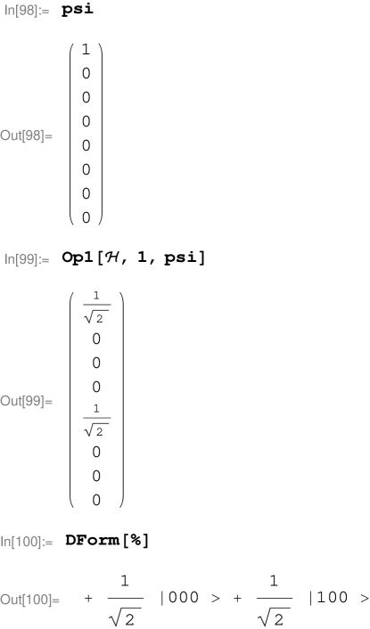
Figure 1: One Hadamard example. Here psi$=\mid 000\rangle.$

One can act with Hadamards on every qubit, by either repeated use of Op1 Figure 2, or by the command $\Omega$ALL[${\bf\cal{H}}$,psi], which is illustrated in Figure 3. A Dirac type notation is also available as illustrated in Figure 4

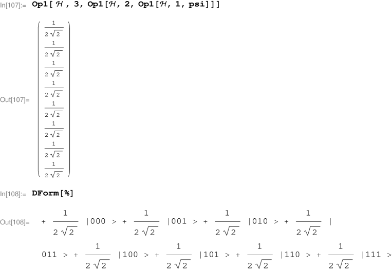
Figure 2: Hadamards on all three qubits example. Here psi$=\mid 000\rangle.$

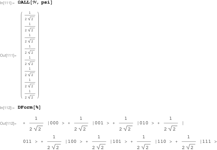
Figure 3: Hadamards on all three qubits using the $\Omega$ALL command. Here psi$=\mid 000\rangle.$

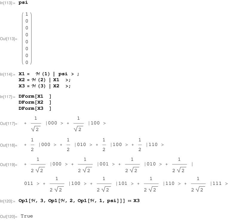
Figure 4: Application of Hadamards in Dirac form. Here psi$=\mid 000\rangle.$

In QCWave.m the command Op1 is given as a Module see Figure 5, which makes use of the command Pick1, Pick1 selects the pairs of decimal labels which differ only in the “is” qubits value of 1 and 0. Then all such pairs are swept through. Examples of Pick1 are presented in the Tutorial.

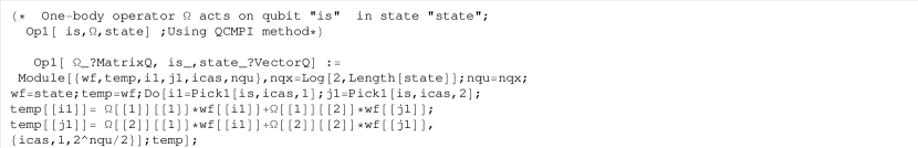
Figure 5: The Op1 command as stipulated in QCWave.m

4.2 Two-qubit operators

The typical two-qubit operators are the CNOT, and controlled phase operators. General two-qubit operators can be constructed from tensor products of two Pauli operators, as discussed earlier. An example from QCWave of application of a CNOT gate is presented in Figure 6.

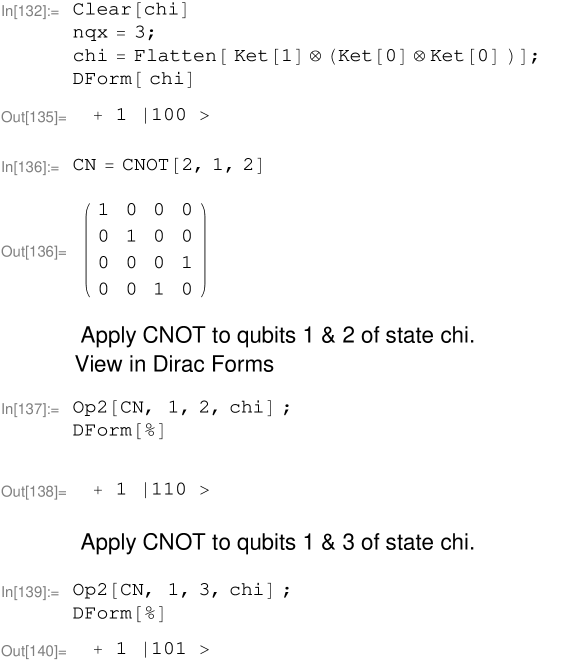
Figure 6: Use of Op2 to apply CNOT gates.

A Dirac type notation is also available as illustrated in Figure 7

Figure 7: Application of CNOT gates in Dirac form.

In QCWave.m the command Op2 is given as a Module see Figure 8, which makes use of the command Pick2, Pick2 selects the quartet of decimal labels which differ only in the ”is1” and ”is2” qubit’s values of 1 and 0. Then all such quartets are swept through. Examples of Pick2 are presented in the Tutorial.

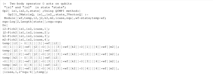
Figure 8: The Op2 command as stipulated in QCWave.m.

4.3 Three-qubit operators

The Op3 command is also provided in QCWave.m as a Module, which makes use of the command Pick3, Pick3 selects the octet of decimal labels which differ only in the ”is1,” ”is2,” and ”is3” qubit’s values of 1 and 0. Then all such octets are swept through. Application to the Tofolli gate is provided in the Tutorial.

5 THE MULTIVERSE APPROACH

5.1 General remarks

Mathematica 7.0 & 8.0 provide a master-slave parallel processing facility. This is not a full implementation of a parallel processing setup that allows communication between the “slave” processors”, such as used by the MPI [9] protocol. If MPI were readily available in Mathematica then one could invoke the full capabilities discussed in QCMPI. That capability allows for the state vector to be distributed over several processors which increases the number of qubits that could be simulated. It is indeed possible to have Mathematica upgraded to include MPI slave to slave communication; as is available in the “POOCH” [10] package. However, since that is an expensive route and most Mathematica users do not have access to MPI, although one can hope for such a capability in the future, we have not invoked the full state distribution aspect.

Nevertheless, the master-slave Mathematica 7.0 capability does provide for concurrent versions of a QCWave based algorithm to be run with different random error scenarios. Then an ensemble averaged density matrix can be formed which describes a real error prone QC setup. That opens the possibility of examining the role of errors and the efficacy of error correction methods using Mathematica.

Therefore, we provide a sample of a parallel setup using some simple basic algorithms, where the parallel setup is described and explained in detail. The following steps are needed: (1) set up your Mathematica code to access several processors, see Appendix 1 for some help; (2) identify the processor number; (3) introduce random errors depending on the processor number; (4) assign a probability distribution for the various processors; (5) form an ensemble average over the processors and store that information as a density matrix on the master processor; (6) repeat these steps including, the algorithm, noise and finally error correction (EC) steps on all processors; (7) examine the resultant density matrix and its evolution to test the EC efficacy. This is an important program that we start by providing simple examples.

A quantum system can evolve in many ways. Different dynamical evolutions are called paths [12] or histories [13]. We refer to these alternate evolutions as separate “universes” and a collection of such possibilities as a multiverse or ensemble of paths. Parallel processing provides a convenient method for describing such alternate paths.

5.2 The ideal and the noisy channels

In our application, we assume that the main path follows an ideal algorithm exactly and the alternate paths incorporate the algorithm with possible noise. That noise is described by random one-qubit operators acting once, or with less likelihood twice. To describe this idea, which is realized in the notebooks MV1-Noise.nb, MV2-Noise.nb and MVn-Noise.nb, consider an initial density matrix $\rho_{0}.$ For a pure state, $\rho_{0}=\mid\psi_{0}\rangle\langle\psi_{0}\mid,$ but it can be a general initial density matrix subject only to the conditions $\rho^{\dagger}=\rho$ and $Tr[\rho]=1.$ The density matrix has $2^{2n_{q}}-1$ parameters and $2^{n_{q}}$ real eigenvalues $\lambda_{n}\leq 1$ with $\sum_{n}\lambda_{n}=1.$ The simplest one-qubit case has the form $\rho=\frac{1}{2}(1+\vec{P}\cdot\vec{\sigma}),$ where the real polarization vector $\vec{P}=Tr[\vec{\sigma}\rho],$ is within the “Bloch sphere”, $(\vec{P}\cdot\vec{P})\leq 1.$ 

5.2.1 Storage case

Consider a simple case where the ideal algorithm is simply leaving the state, as described by $\rho_{0},$ alone. This is a memory storage case. Ideally, $\rho$ remains fixed in time. Assume however that this ideal case occurs with a probability $\texttt{p}\lesssim 1$ and that alternate evolutions occur with a probability $\epsilon=1-\texttt{p}.$ For example, we take $\texttt{p}=.8$ and $\epsilon=.2,$ corresponding to a 80% perfect storage and 20% possibility of noise. We also assume for more than 1 qubit cases that 95% of the 20% noise ($.2\times.95\rightarrow 19\%$) involves a single one-qubit hit, while 5% of the 20% noise ($.2\times.05\rightarrow 1\%$) involves two one-qubit hits.

The ensemble average over all paths then yields a density matrix

$$\rho_{f}=\texttt{p}\ \rho_{0}+\frac{\epsilon}{n_{p}}(\Omega^{(1)}\ \rho_{o}\ \Omega^{(1)\dagger}+\Omega^{(2)}\ \rho_{o}\ \Omega^{(2)\dagger}\cdots\Omega^{(n_{p})}\ \rho_{o}\ \Omega^{(n_{p})\dagger}),$$ (45)

where the operators $\Omega^{(1)},\Omega^{(2)}\cdots\Omega^{(n_{p})}$ act in each of the $n_{p}$ paths with a probability $\frac{\epsilon}{n_{p}}.$ Each of these $n_{p}$ terms is evaluated on a separate processor, so that $n_{p}$ equals the total number of processors invoked. The above ensemble average preserves the trace:

$$Tr[\rho_{f}]=\texttt{p}\ Tr[\rho_{0}]+\frac{\epsilon}{n_{p}}\sum_{n=1}^{n=n_{p}}{Tr[\Omega^{(n)}\ \rho_{o}\ \Omega^{(n)\dagger]}}=\texttt{p}+\frac{\epsilon}{n_{p}}n_{p}=1.$$ (46)

Here we assume that each $\Omega^{(n)\dagger}\Omega^{(n)}=1,$ and hence that $Tr[\Omega^{(n)}\ \rho_{o}\ \Omega^{(n)\dagger}]=Tr[\rho_{o}\ ]=1.$ In addition, $\rho_{f}^{\dagger}=\rho_{f}.$

This multiuniverse approach is illustrated in Figure 9. For the pure storage case the algorithm operators $\Omega_{A},\tilde{\Omega}_{A}\cdots$ are all set equal to unit operators. See later for a simple non-trivial case.

Figure 9: The multiverse approach. Each curve represents a possible evolution of a quantum system of $n_{q}$ qubits. The solid curve represents the main evolution path, with probability $\texttt{p}.$ The dotted curves represent the $n^{th}$ evolution path, with probability $\frac{\epsilon}{n_{p}}.$ The initial density matrix is $\rho_{0}$ and the final $\rho_{F}.$ The unitary noise operators $\Omega^{(i)}$ act on each path $i.$ Here $\tilde{\Omega}^{(i)}$ denote subsequent noise operators. The operators $\Omega_{A}$ and $\tilde{\Omega}_{A}$ denote the $n_{q}$ algorithm operators which act on all paths.

5.2.2 Multiverse and POVM

The above representation can also be cast in the POVM (Positive Operator Valued Measure) and Kraus operator form. The evolution can be expressed as

$$\rho_{f}=\sum_{n=0}^{n=n_{p}}\ \tilde{\Omega^{n}}\ \rho_{0}\ \tilde{\Omega}^{n\dagger},$$ (47)

where we define $\tilde{\Omega}^{0}=\sqrt{\texttt{p}}\ \mathbf{1},$ and $\tilde{\Omega}^{n\rangle 0}=\sqrt{\frac{\epsilon}{n_{p}}}\Omega^{n}.$ This is the form known as POVM, which can be deduced [14] from embedding a quantum system in an environment, which is then projected out. This evolution form can also be used to deduce the Lindblad [15] equation for the evolution of a density matrix subject to environmental interactions. Here we arrive at these forms from a simple multiuniverse approach.

5.2.3 Multiverse and classical limit

Our task is to set up this multiuniverse approach using the parallel, multi-processor features of Mathematica. Equation 45 describes the evolution of a density matrix after one set of operators act in the various possible paths. A subsequent set of operators is described by

$$\rho_{F}=\texttt{p}\ \rho_{f}+\frac{\epsilon}{n_{p}}\sum_{n=1}^{n=n_{p}}({\vtop to0.0pt{\hbox{\lower 7.0pt\hbox{$\hat{\vphantom{.}}$}} \vss}}{\Omega}^{(n)}\ \rho_{f}\ \Omega^{(n)\dagger}).$$ (48)

As this evolution process continues to be subject to additional noise operators, the density matrix evolves into a diagonal or classical form. In this way the noise yields a final classical density matrix with zero off-diagonal terms; this is the decoherence caused by a quantum system interacting with an environment. If the qubit states are not degenerate and the noise is of thermal distribution, the density matrix in the classical limit will evolve towards the thermodynamic form $\exp(-\frac{H}{kT}).$ At every stage, one can track the von Neumann entropy( $S(\rho)=-Tr[\rho\ln[\rho]]),$ the Purity ( $Tr[\rho\cdot\rho]),$ and the Fidelity ( $F[\rho,\rho_{0}]=Tr[\sqrt{\sqrt{\rho_{0}}\ \cdot\rho\cdot\ \sqrt{\rho_{0}}}]),$  of the system. In addition, the eigenvalues of the system can be monitored where in the classical limit the eigenvalues all approach $\frac{1}{2^{n_{q}}},$ and the entropy goes to $S[\rho]\rightarrow n_{q}.$ Subsystem entropy and eigenvalues can also be examined.

5.3 Multiverse algorithms and errors

The evolution of the density matrix, with noise included via the multiverse approach on the available processors, can also be implemented when an algorithm is included. The procedure is to act with the algorithm gate operators after each ensemble averaged density matrix is formed. The explicit expression is given in Equation 45 which for the $nth$ step is

$$\rho_{n+1}=\Omega_{A}\ \left[\rho_{n}\ +\frac{\epsilon}{n_{p}}\ \sum_{k=1}^{k=n_{p}}\ \ \sum_{s=1,2}\ p_{s}\Omega_{ks}\rho_{n}\Omega_{ks}^{\dagger}\ \right]\ \Omega_{A}^{\dagger}$$ (49)

where $\Omega_{A}$ are the gates for the specific algorithm and $\Omega_{ks}$ are the noise operators on the $kth$ processor for two cases, $s=1$ denotes a one qubit noise operator hitting one qubit and $s=2$ denotes one qubit operators hitting two separate qubits. The factors $p_{k}$ are assumed to be $p_{1}=.95$ and $p_{2}=.05,$ so that the one-qubit hits have a net probability ($\epsilon*p_{k}$) of 19% and the double hit case a net probability of 1%. The algorithm operators $\Omega_{A}$ are applied to all all processors, but implemented by evaluation on the master processor.

In QCWAVE, the above steps are implemented in the notebooks MV1-Noise, MV2-Noise and MVn-Noise, for systems consisting of 1,2, or $n$ qubits. The key step is shown in Figure 10, where denE[n] denotes the ensemble averaged density matrix at stage $n$, and the parallel part of the command distributes the evaluation of the noise over the “nprocs” processors, which is doubled to account for the “s” label in Equation 49.

Figure 10: Here denE[0[] is the initial density matrix $\rho_{0}$ and denE[nv] denotes the ensemble averaged density matrix after nv steps. The algorithm operators “OPA[nv]” are setup within the code, and the noise operators OP[ i , nv ] act on the $i^{th}$ processor at the $nv^{th}$ step. These noise operators are held fixed after they are randomly generated.

A simple algorithm is illustrated in MV1-Noise; namely, one starts with the state $\mid 0\rangle$ which is then hit by a Hadamard ${\bf\cal{H}},$ and after an interlude of noise, another Hadamard hits, followed by a long sequence of noise. Without noise this process correspond to a rotation to the x-axis and then a rotation back to the z-axis. One also sees the polarization vector rotated, rotated back and then, after a sequence of noise hits, decay to zero and density matrix then evolves into a diagonal form, with both eigenvalues equal to 1/2. How is this simple process affected by noise during these steps? To answer that question the entropy, purity and fidelity evolution are tracked. The results from MV1-Noise are illustrated in Figure 11.

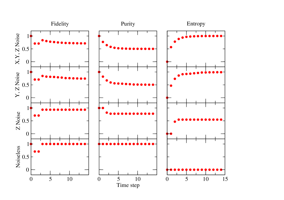
Figure 11: The fidelity (left column), purity (central column) and entropy (right column) evolution is displayed for one qubit initially in a state $\mid\psi_{0}\rangle=\mid 0\rangle,$ that is subject to a Hadamard at step 1 and another Hadamard at step 3, for various noise scenarios. The top plot is for X,Y and Z noise, the next plot down has Y and Z noise, and the next Z-noise only. The bottom plot is the noiseless channel, for which the fidelity returns to one, after dropping to $1/\sqrt{2},$ which clearly reflects the action of 2 sequential Hadamards.

Another simple algorithm is illustrated in MV2-Noise; namely, one starts with the state $\mid 00\rangle,$ qubit one is then hit by a Hadamard ${\bf\cal{H}},$ and after an interlude of noise, a CNOT gate acts on both qubits. This is the algorithm for producing a Bell state CNOT${}_{1,2}{\cal H}_{1}\mid 00\rangle=\frac{1}{2}(\mid 00\rangle+\mid 11\rangle).$ This is followed by an inverse Bell operator ${\cal H}_{1}$CNOT${}_{1,2},$ and then a long sequence of noise. The density matrix then evolves into a diagonal form, with all 4 eigenvalues equal to 1/4. The two polarizations, and the spin correlations are displayed along with the evolution of the eigenvalues, the entropy, purity and fidelity. The results from MV2-Noise are illustrated in Figures 12.– LABEL:MV2ENT.

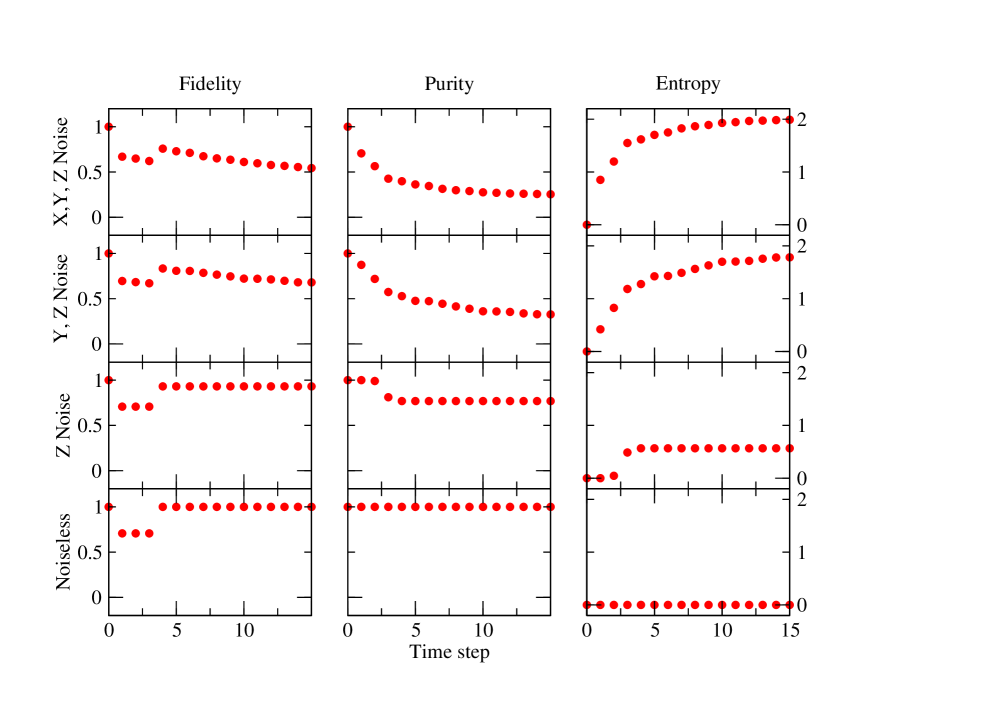
Figure 12: The fidelity (left column), purity (central column) and entropy (right column) evolution is displayed for two qubits initially in a state $\mid\psi_{0}\rangle=\mid 00\rangle,$ that is subject to a CNOT${}_{12}{\cal H}_{1}$ and later a ${\cal H}_{1}$CNOT₁₂, for various noise scenarios. The top plot is for X,Y and Z noise, the next plot down has Y and Z noise, and the next Z-noise only. The bottom plot is the noiseless channel, for which the fidelity returns to one, after dropping to $1/\sqrt{2},$ which clearly reflects the action of the 2 sequential operators.

Clearly, more sophisticated algorithms can be invoked. We next consider how to monitor and correct for the noise.

5.4 Multiverse and error correction

5.4.1 Simulation of error correction

Error correction (EC) typically involves encoding the qubits using extra qubits, then entangling those encoded qubits with auxiliary qubits. Measurements are made on the auxiliary qubits, so as not to disturb the original encoded qubits. Those measurements provide information as to whether an error has occurred, its nature and where it acted. Hence a remedial gate can be applied to undo the error. If desired, the encoded qubits can then be decoded and the original error-free qubit restored. That process is illustrated for simple X and Y errors on one qubit EC and for Shor’s 9 qubit EC code in notebooks EC3x, EC3z and Shor9Tutorial. More sophisticated EC codes are available in the literature, along with a general theoretical framework [16]. This kind of EC has to be constantly invoked as an algorithm evolves, which is a rather awkward and qubit-costly process. Error in the gates themselves is an additional concern, usually one assumes perfect gates, with errors (noise) occurring only in-between application of the gates.

For our purpose, instead of applying the procedures outlined in the above EC notebooks, we simulate EC by a rather simple procedure. In the notebooks, the operators ss[i] are set equal to the Pauli operators s[i] to generate noise. By replacing ss[1] by s[0] (the $2\times 2$ unit operator), all X-noise is turned off “by hand.” Then a rerun is generated which has the same structure as with the noise, except the X-noise has been removed. Similar steps can be used to remove the Y and the Z-noise operators. In that way a set of results can be generated ranging from a full noise, to partial noise to no noise cases. Examples from MV1-noise and MV2-noise are presented in Figures 11and 12.

If the user wishes to invoke other noise operators, that can be accommodated as well. For example, a general unitary random rotation can be used as a noise operator by invoking the form shown in Figure 13. Thus ”ss[4] =UE1” is used to turn on such rotations. Replacing s[4] to s[0] again provides a way to turn this operator off to remove that noise element.

Figure 13: This is an option to use a general rotation as the noise operator as an alternative to the Pauli operators. The s[4] location can be used to include this option.

With this simple scheme, one can study many more noise and EC scenarios. For example, in the notebook MVn-Noise the case of an algorithm for 5 qubits is presented. The algorithm consists of a Hadamard followed by a CNOT chain, i.e. CNOT₁₅ CNOT₁₄ CNOT₁₃ CNOT${}_{12}{\cal H}_{1}\mid 00\rangle.,$ including noise in-between and after the 9th step. Detailed examination of the entropy, fidelity, purity and eigenvalues and noise is presented within that notebook. Of particular interest is the EC simulation results when the noise operators are turned of sequentially.

6 ADDITIONAL FEATURES

6.1 Amplitude displays

The amplitude coefficients $C_{n}$ can be displayed in various ways using the commands Amplitudes and MeterGraph as illustrated in Figure LABEL:amps

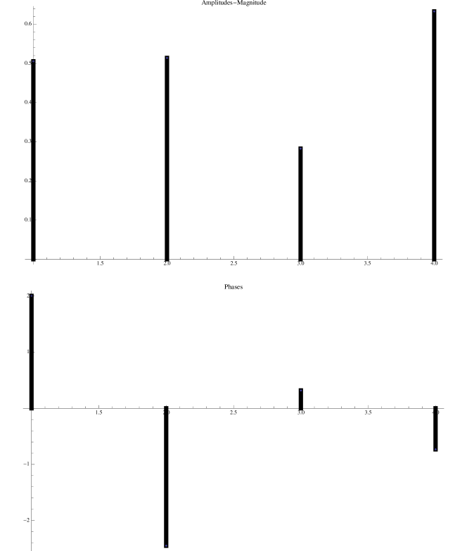
Figure 14: Amplitudes command displays amplitudes as magnitude and phase bar graphs.–see QCWave.m

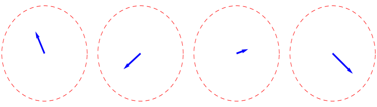
Figure 15: MeterGraph displays amplitudes as argand plots–see QCWave.m

6.2 Dirac form

The command DForm has already been demonstrated in Figures 1–4,and 6. Another Dirac form has be invoked in QCWAVE as shown in Figure 4. A more extensive Dirac notation scheme has been provided by José Luis Gómez-Muñoz et al. in Ref. [3].

6.3 Circuit diagrams

Illustrations of circuit drawing are included throughout the notebooks, with the CircuitTutorial notebook providing an overview. The commands are all defined in Circuits.m. One example is given in Figure 16.

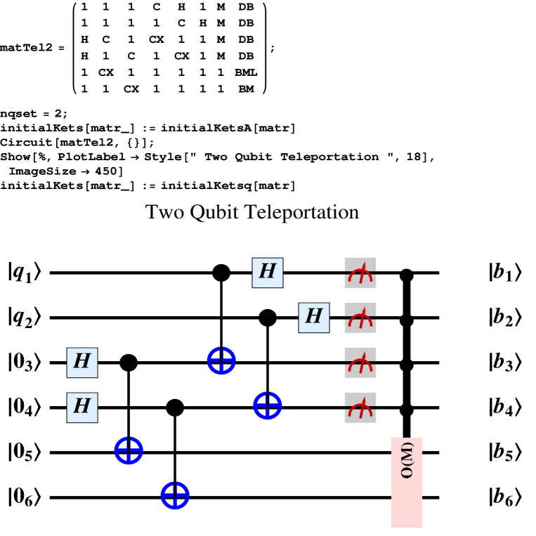
Figure 16: A sample circuit diagram as produced in notebook TeleportationW is shown here. The initialKetsA sets the initial array sequence as: $\mid q_{1}\rangle,\mid q_{2}\rangle,\mid 0_{3}\rangle\cdots\mid 0_{6}\rangle.$

6.4 Upgraded applications

Upgraded versions of Grover [17], Teleportation [18] and Shor [19] algorithms are included in the present version.

7 CONCLUSION & FUTURE APPLICATIONS

This package will hopefully be instructive and useful for applications to error correction studies. Hopefully users will contribute to improvements and extensions and for that purpose we are developing an interacting web page. When MPI becomes available on Mathematica, there will be another opportunity to upgrade QCWAVE to a full research tool.

Application to explicit quantum computing problems, such as study of non-degenerate states and the associated phase factors, errors in gates themselves (where the gates are produced by explicit pulses), and the direct application of EC schemes are among the possible future applications. Novel EC schemes, such as stabilizing pulses or EC stable spaces could be additional fruitful applications.

Appendix A Setting up Processors with Mathematica

In order to use parallel processing with Mathematica, one needs to first gain access to several processors. There are other ways to do this, but, the commands we used are given in Figure 17. Note that the user need to be sure that the ssh (secure shell) access is working and accesses the Mathematica command on the other machines (which could be Macs or PCs or a combination of them).

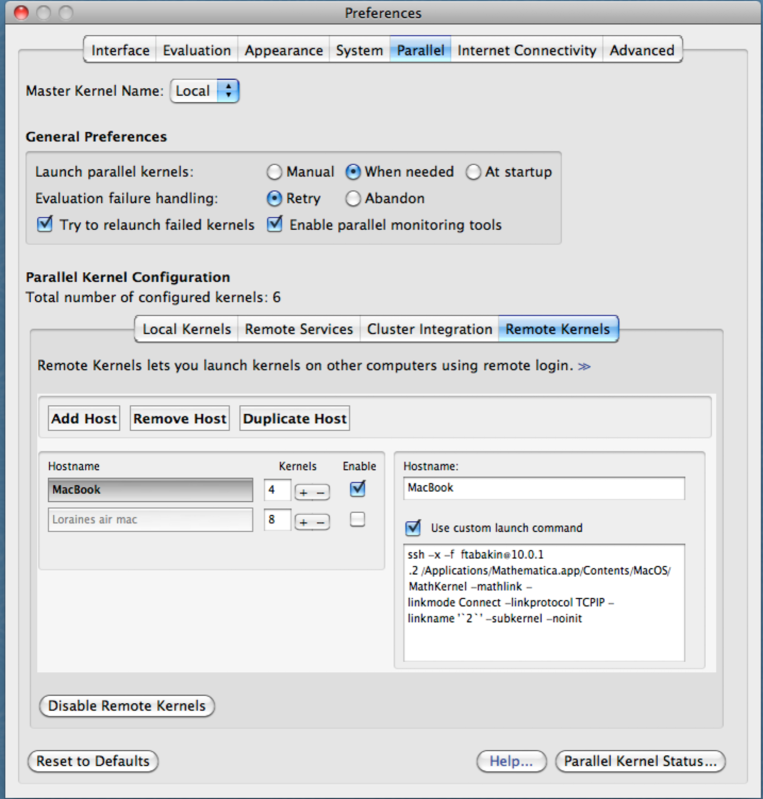
Figure 17: The preferences setup to access other processors– use “Evaluation/Parallel Kernel Configuration/Remote Kernels” to get to this page. You also need to set the Local Kernels entry. The user also needs to establish an ssh link to the other machines and be sure it properly accesses the Mathematica installed on all processors.

In addition, one needs to setup the basic programs and requisite packages on all the processors used. For that the initializations shown in Figure 18 are needed.

Figure 18: The commands needed to invoke the packages on parallel processors. QCWave.m and Circuits.m are add-ons to the original QDensity.m package.

References

- [1] Bruno Juliá-Díaz, Joseph M. Burdis and Frank Tabakin, “QDENSITY - A Mathematica Quantum Computer simulation,” Comp. Phys. Comm., 174 (2006) 914-934. Also see: Comp. Phys. Comm.,1 80, (2009) 474 and http://www.pitt.edu/ tabakin/QW/, for our QCWAVE webpage.
- [2] See http://www.wolfram.com/mathematica/ .
-
[3]
José Luis Gómez-Muñoz,”A free Mathematica
add-on for Dirac Bra-Ket Notation, Quantum Algebra and
Quantum Computing,”
http://homepage.cem.itesm.mx/lgomez/index.htm. -
[4]
J. Lapeyre,
“Qinf quantum information and entanglement package for the Maxima computer
algebra system”,
http://www.johnlapeyre.com/qinf/index.html. - [5] Frank Tabakin and Bruno Juliá-Díaz, “QCMPI: A parallel environment for quantum computing”, Comp. Phys. Comm., 180 (2009) 948-964.
- [6] P. A. M. Dirac, “The Principles of Quantum Mechanics”, Oxford University Press, USA 4th ed. ISBN: 0198520115.
- [7] Albert Messiah, “Quantum Mechanics” , Dover Publications , ISBN : 0486409244.
- [8] Michael A. Nielsen and Isaac I. Chuang, “Quantum Computation and Quantum Information”, Cambridge University Press (2000).
- [9] See: http://www.open-mpi.org/ .
-
[10]
A Mathematica MPI code is available at
http://daugerresearch.com/index.shtml. - [11] CLOJURATICA is available at http://clojuratica.weebly.com/index.html. It combines the advantages of Mathematica with the Clojure language and “includes a concurrency framework that lets multiple Clojure threads execute Mathematica expressions without blocking others…” .
- [12] R. P. Feynman and A. R. Hibbs, “Quantum Mechanics and Path Integrals”, New York: McGraw-Hill, (1965).
- [13] R. B. Griffiths, “Consistent Quantum Theory”, Cambridge University Press, (2003).
-
[14]
John Preskill, “Lecture Notes on quantum information
and computation”, available at,
http://www.theory.caltech.edu/people/preskill/ph229/, see: Chapter 3.2-3.5. - [15] G. Lindblad, Comm. Math. Phys. 4 ,119 (1976).
- [16] D. Gottesman, “A Theory of Fault-Tolerant Quantum Computation,” Phys. Rev. A 57, 127-137 (1998), quant-ph/9702029.
- [17] L. K. Grover, Phys. Rev. Lett. 79, 325-328 (1997).
- [18] C. H. Bennett, G. Brassard, C. Crépeau, R. Jozsa, A. Peres, and W. K. Wootters, Phys. Rev. Lett. 70, 1895-1899 (1993).
- [19] Peter W. Shor, SIAM J. Comput. 26 (5): 1484 (1997).