Spectral density of the Hermitean Wilson Dirac operator: a NLO computation in chiral perturbation theory

Abstract

We compute the lattice spacing corrections to the spectral density of the Hermitean Wilson Dirac operator using Wilson Chiral Perturbation Theory at NLO. We consider a regime where the quark mass $m$ and the lattice spacing $a$ obey the relative power counting $m\sim a\Lambda_{\rm QCD}^{2}$: in this situation discretisation effects can be treated as perturbation of the continuum behaviour. While this framework fails to describe lattice spectral density close to the threshold, it allows nevertheless to investigate important properties of the spectrum of the Wilson Dirac operator. We discuss the range of validity of our results and the possible implications in understanding the phase diagram of Wilson fermions.

I Introduction

Simulations with Wilson fermions at light quark masses are nowadays feasible thanks to considerable algorithmic improvements Hasenbusch and Jansen (2003); Luscher (2005); Urbach et al. (2006); Clark and Kennedy (2007); Luscher (2007) developed in the last years. Since chiral symmetry is explicitly broken, the spectrum of the Wilson Dirac operator is not protected from arbitrarily small eigenvalues, which might induce instabilities in numerical simulations Del Debbio et al. (2006). It is therefore very important to have a theoretical understanding of the properties of the low-end spectrum of the Wilson Dirac operator. Moreover, spectral observables can be efficiently used to extract relevant quantities such as the quark condensate, like recently implemented in Giusti and Luscher (2009), yielding a further strong motivation to investigate the impact of lattice artefacts on the eigenvalues spectrum.

In the continuum and in an infinite volume, the (renormalised) spectral density of the massive Dirac operator has a threshold given by the (renormalised) quark mass. Lattice artefacts are expected to change both the location of the threshold and the shape of the spectral density close to the threshold. Moreover, in a finite box of volume $V$ one expects that when $\gamma\Sigma V\simeq 1$, where $\gamma$ is an eigenvalue of the massless Dirac operator and $\Sigma$ the chiral condensate, finite-size effects become important and can also induce relevant deformations of the spectral density with respect to the infinite-volume case.

From the numerical point of view, some information about the low-end spectrum is provided by lattice simulations with Wilson fermions carried out in the past years. For $N_{f}=2$ unimproved Wilson fermions, empirical observations Del Debbio et al. (2006) indicate that the median of the spectral gap distribution is linearly proportional to the quark mass $m$, while the width is basically independent on $m$ and scales like $\sim a/\sqrt{V}$, where $a$ is the lattice spacing. On the other hand, for the $O(a)$-improved theory, the situation is less clear Del Debbio et al. (2007) and those properties have not been confirmed. In Giusti and Luscher (2009) the mode number of the $O(a)$-improved Wilson Dirac operator is computed, finding a nearly linear behavior up to $\simeq 100$ MeV above the threshold. At the low end of the spectrum, a significant deviation from the continuum expectation is observed.

From the theoretical side, Wilson chiral perturbation theory Sharpe and Singleton (1998); Rupak and Shoresh (2002) (W$\chi$PT) is the tool which provides a systematic description of low-energy properties of lattice Wilson QCD including the leading discretisation effects. When approaching the chiral limit at finite lattice spacing, one enters in the regime where $m\sim a^{2}\Lambda_{\rm QCD}^{3}$, which is where discretisation effects compete with the quark mass to the explicit breaking of chiral symmetry. Lattice artefacts induce a non-trivial phase diagram, and two different scenario have been foreseen: in the so-called Aoki scenario there is a range of quark masses (in the Aoki phase Aoki (1984)) where there are two massless pions. On the other hand, in the so-called Sharpe-Singleton scenario Sharpe and Singleton (1998) there is a first-order phase transition, and the three pions remain massive in the chiral limit. From the point of view of W$\chi$PT, in this regime the discretisation effects appear already at leading order in the chiral expansion. Lattice artefacts in the infinite volume spectrum of the Hermitean Wilson Dirac operator have been computed in this regime in Sharpe (2006), although a working framework has been only found by assuming additional conditions on the couplings of W$\chi$PT associated to discretization effects.

In a recent study Damgaard et al. (2010); Akemann et al. (2010) the same power counting for $a$ has been adopted, but in a finite-box in the $\epsilon$-regime. In this case the LO predictions of W$\chi$PT can be obtained also by means of a “modified” Random Matrix Theory which includes $O(a^{2})$ effects. The main difficulty of this computation is that it involves exact integrals over the zero modes which must be defined at fixed topological charge introduced via the number of real modes of the Dirac operator, which nevertheless has an intrinsic ambiguity for Wilson fermions at finite lattice spacing.

In this work we will study the discretisation effects in the spectrum of the Dirac operator in a different regime. We consider W$\chi$PT with the power counting $m\sim a\Lambda_{\rm QCD}^{2}$ (GSM regime), where lattice artefacts appear only at next-to-leading order in the chiral effective theory, and can hence be treated as a perturbation. This simplifies considerably the computation; it allows nevertheless to extract important information about the impact of lattice artefacts in the spectral density.

This paper is structured as follows: in sec. II we recall definitions and properties of the spectral density of the Wilson Dirac operator; in sec. III we present the setup for W$\chi$PT needed for the computation; in sec. IV we give the details about the calculation of the spectral density, including the finite-volume corrections (in the $p$-regime); in sec. V we discuss our results and show a comparison with numerical data. All technical details about the computation are deferred in the Appendices.

II Spectral density for the Wilson Dirac operator

We start considering QCD for $N_{f}=2$ degenerate quarks in infinite volume with current quark mass $m$. The average spectral density of the massless Hermitian Dirac operator $-iD$ can be defined as

$$\rho_{D}(\gamma,m)\equiv\lim_{V\rightarrow\infty}\frac{1}{V}\sum_{k}\langle\delta\left(\gamma-\gamma_{k}\right)\rangle,$$ (1)

where $\gamma_{k}$ are the eigenvalues of the massless Hermitian Dirac operator and $\langle\ldots\rangle$ indicates the usual path-integral average. The Banks-Casher relation Banks and Casher (1980) tells us that the spectral density is related to the chiral condensate $\Sigma$ in the following way

$$\rho_{D}\left(\gamma,m\right)=\frac{\Sigma}{\pi}\left[1+O(\{|\gamma|,m\}/\Lambda_{QCD})\right].$$ (2)

One useful way to determine this relation in continuum QCD Chandrasekharan (1995); Verbaarschot (1996) consists in adding a valence quark $\psi_{v}$ of mass $m_{v}$ to the theory. Using the spectral decomposition for the valence chiral condensate one obtains

$$\langle\overline{\psi}_{v}\psi_{v}\rangle=-\int d\gamma\frac{\rho_{D}(\gamma,m)}{i\gamma+m_{v}}.$$ (3)

This relation can be inverted because the spectral density is independent on the valence quark mass

$${\rm Disc}\left[\langle\overline{\psi}_{v}\psi_{v}\rangle\right]{\large|}_{m_{v}=-i\gamma}=-2\pi\rho_{D}(\gamma,m),$$ (4)

where ${\rm Disc}$ indicates the discontinuity across the imaginary valence quark mass. Strictly speaking eq. (3) is ultraviolet divergent also after renormalisation of the quark masses and the gauge coupling constant and one must introduce a cutoff in the integration range. The ultraviolet divergences turn out to cancel when computing the discontinuity of the valence scalar condensate in eq. (4). Thus it is enough to compute the valence condensate for real masses and analytically continuing the resulting expression for complex masses. Eq. (4) can be used naturally in chiral perturbation theory and one obtains Verbaarschot (1996) the Banks-Casher relation (2) and the NLO corrections Osborn et al. (1999); Giusti and Luscher (2009).

We now discretise our $N_{f}=2$ continuum QCD action on a lattice of spacing $a$ and we consider Wilson fermions. All our considerations can be generalised to the case of Wilson twisted mass. To study the spectral density of the Wilson operator one has to take into account that the Wilson operator $D_{W}$ is neither Hermitian nor anti-Hermitian and it has complex eigenvalues. It is thus advantageous to define the Hermitian Wilson-Dirac operator $Q_{m}$

$$Q_{m}=\gamma_{5}\left(D_{W}+m\right)=Q_{m}^{\dagger}.$$ (5)

We indicate now the spectral density of $Q_{m}$ as $\rho_{Q}(\lambda,m)$ and the one of $Q_{m}^{2}$ as $\rho(\alpha,m)$, where $\lambda$ and $\alpha$ label the eigenvalues of the corresponding operators.

If the continuum theory has been regulated on a lattice the ultraviolet divergences of the chiral condensate appear as power law and logarithmic divergences in the lattice spacing $a$. Moreover, when using Wilson fermions the lack of chiral symmetry implies that the scalar condensate is not directly related to the spectral density as in the continuum. It is thus not obvious how to work out the renormalisation and O($a$) improvement of the spectral density starting from eq. (4) or from the corresponding version for Wilson lattice QCD. To study the renormalisation and the O($a$) improvement of the spectral density one needs to relate it to correlation functions of local operators where standard arguments on renormalisability and O($a$) improvement can be applied.

It has been shown in ref. Giusti and Luscher (2009), using chain correlators of scalar and pseudoscalar densities how the spectral density of $Q_{m}^{2}$ renormalises. In the following we will be mostly interested in the spectral density of $Q_{m}$ that renormalises as follows

$$\left[\rho_{Q}\right]_{R}(\lambda,m_{R})=Z_{P}\rho_{Q}(Z_{P}\lambda,m),$$ (6)

where $m_{R}$ is the renormalised quark mass. Moreover, additionally to the standard improvement of the action and local operators there are O($am$) cutoff effects which need to be removed to fully improve the spectral density Giusti and Luscher (2009). This analysis guarantees that with Wilson fermions the spectral density is a well defined renormalisable quantity and with a well defined Symanzik expansion. We can thus compute the spectral density in the chiral effective theory using a generalisation of eq. (4) for Wilson chiral perturbation theory.
A further spectral observable which can be defined and measured in a lattice simulation is the integrated spectral density

$$N(\Lambda_{1},\Lambda_{2},m)=\int_{\Lambda_{1}}^{\Lambda_{2}}d\lambda~{}\rho_{Q}(\lambda,m),\;\;\;\;\Lambda_{2}\geq\Lambda_{1}\geq m,$$ (7)

which represents the density of modes in the interval between $\Lambda_{1}$ and $\Lambda_{2}$; it contains the same physical information as the spectral density and satisfies $N_{R}(\Lambda_{1,R},\Lambda_{2,R},m_{R})=N(\Lambda_{1},\Lambda_{2},m)$, i.e. it is a renormalisation-group invariant Giusti and Luscher (2009).

To relate a partially quenched condensate with the spectral density of $Q_{m}$ it is convenient to introduce a doublet of degenerate twisted mass fermions $\chi_{v}$ with a mass term $i\mu_{v}\gamma_{5}\tau^{3}$, where $\tau^{3}$ is the third Pauli matrix. The relation between the condensate and the spectral density is now different but can be worked out and it reads Sharpe (2006)

$$\langle\overline{\chi}_{v}\gamma_{5}\tau^{3}\chi_{v}\rangle=\int_{-\infty}^{\infty}d\lambda\frac{\rho_{Q}(\lambda,m)+\rho_{Q}(-\lambda,m)}{\lambda+i\mu_{v}}.$$ (8)

The need to symmetrise in $\lambda$ the spectral density in the numerator of (8) can be understood from the lack of chiral symmetry of the Wilson operator which renders the spectral density not symmetric when $\lambda\rightarrow-\lambda$. Inverting eq. (8) one obtains

$${\rm Disc}\left[\langle\overline{\chi}_{v}\gamma_{5}\tau^{3}\chi_{v}\rangle\right]|_{\mu_{v}=i\lambda}=2i\pi\left[\rho_{Q}(\lambda,m)+\rho_{Q}(-\lambda,m)\right]\,$$ (9)

where the untwisted mass in the valence sector coincides with the sea quark mass $m$. Eq. (9) is our starting point for the computation of the spectral density in Wilson chiral perturbation theory.

We stress that in chiral perturbation theory the problem of power law divergences is absent because those are mapped to the presence of the so called high-energy constants usually indicated with $H$. As we will see in sect. IV this is indeed the case for the expectation value of the pseudoscalar condensate in the chiral effective theory. This implies that in the effective theory the computation of the discontinuity is a well defined procedure. It remains to make sure that the spectral density computed in the effective theory through the discontinuity of the partial quenched chiral condensate does not overlook additional cutoff effects which go beyond the standard O($a$) corrections stemming from the action or the local operators. Our previous discussion and the results of ref. Giusti and Luscher (2009) guarantees that the only additional cutoff effects are of O($am$) and as we will see in sect. III these cutoff effects are of subleading order in our power counting of Wilson chiral perturbation theory.

III Spectral density in Wilson Chiral Perturbation Theory

In order to investigate the discretisation effects in the spectral density of the Hermitian Wilson Dirac operator we compute the valence pseudoscalar density in the framework of Partially Quenched Wilson chiral perturbation theory (PQW$\chi$PT). According to eq. (8), we consider $N_{f}=2$ sea quarks with bare mass $m$ and a doublet of valence twisted mass quarks with $(m+i\mu_{v}\tau^{3})$. We formulate the effective theory on a finite volume $V=L^{3}T$ and we keep the quark masses in the $p$-regime, corresponding to the power counting

$$m,\mu_{v}\sim O(p^{2}),\;\;\;1/L,1/T\sim O(p)$$ (10)

in terms of the momenta $p$. The extension of the effective theory to the case of non-zero lattice spacing is done in two steps: after matching the lattice QCD action with the appropriate Symanzik continuum effective action Symanzik (1983a, b), one writes down a chiral Lagrangian which contains the standard continuum terms plus additional operators that transform under chiral symmetry as the operators of the Symanzik effective theory. For the Wilson action, this has been studied in Sharpe and Singleton (1998); Rupak and Shoresh (2002). When introducing lattice artefacts in the chiral effective theory, we have to define as usual the relative power counting between the quark mass and the lattice spacing $a$. In this work we adopt a counting corresponding to the so-called GSM (Generically Small quark Mass) regime Sharpe and Wu (2004, 2005), where $m,\mu_{v}\sim a\Lambda_{\rm QCD}^{2}$: in this case the explicit breaking of chiral symmetry is dominated by the quark mass, and lattice artefacts can be treated as perturbations.

Partially quenching can be implemented in the Chiral Effective theory by means of two techniques, namely the graded-symmetry method Bernard and Golterman (1992, 1994) and the replica method Damgaard and Splittorff (2000). In the first one, one introduces “ghost” quarks, whose determinant cancels the one of the valence quarks. In the second one, one enlarges the valence sector to $N_{r}$ flavors and one eliminates the corresponding determinant by sending $N_{r}\rightarrow 0$. The equivalence of the two methods has been shown at the perturbative level in Damgaard and Splittorff (2000). In this section we will focus on the graded-symmetry method; we checked nevertheless that the same results can be obtained with the replica method, which we summarise in App. B. For our specific case we have to consider a chiral Effective Theory with a graded symmetry group SU$(4|2)_{L}$$\times$SU$(4|2)_{R}$ spontaneously broken to SU$(4|2)_{R+L}$. The formulation we adopt for our computation using the SU$(4|2)$ effective theory is based on an extension of the framework proposed in Giusti (2008) for the SU$(3|1)$ case. We consider a mass matrix of the form

$$\mathcal{M}={\rm diag}(\underbrace{m}_{2\times 2\;{\rm sea}},\underbrace{m+i\mu_{v}\tau^{3}}_{2\times 2\;{\rm val}},\underbrace{m+i\mu_{v}\tau^{3}}_{2\times 2\;{\rm ghost}}).$$ (11)

The quark mass in the ghost sector has been already set equal to the mass in the valence sector. Moreover, the untwisted part of the valence quark mass has to be equal to the sea quark mass. We parametrise the pseudo Nambu-Goldstone bosons by the field $U\in$ SU$(4|2)$

$$U(x)=u_{V}e^{2i\xi(x)/F}u_{V},\;\;\;\;\xi=\sum_{a}\xi^{a}T^{a},$$ (12)

where $F$ is as usual the pseudoscalar decay constant, and $T^{a},a=1,\ldots,35$ represent the generators of the corresponding Lie algebra, which satisfy

$${\rm Str}(T^{a}T^{b})=\frac{g^{ab}}{2}.$$ (13)

We refer to App. A for the explicit form of $g^{ab}$ (eq. (70)), and for a summary of conventions and properties of the SU$(m|n)$ group. The constant field $u_{V}$ represents the ground state of the theory, which can be obtained by minimising the potential in the LO Chiral Lagrangian. The solution of the potential minimisation yields

$$u_{V}={\rm diag}(\underbrace{1}_{2\times 2\;{\rm sea}},\underbrace{e^{i\tau^{3}\omega_{0}/2}}_{2\times 2\;{\rm val}},\underbrace{e^{i\tau^{3}\omega_{0}/2}}_{2\times 2\;{\rm ghost}}),$$ (14)

where

$$\sin\omega_{0}=\frac{\mu_{v}}{m_{P}},\;\;\;\cos\omega_{0}=\frac{m}{m_{P}},\;\;\;\;m_{P}=\sqrt{m^{2}+\mu_{v}^{2}}.$$ (15)

In the language of twisted mass Wilson theory, $m_{P}$ is the so-called polar mass.

Taking into account our power counting, the full NLO Chiral Lagrangian in PQW$\chi$PT can be written as

$$\mathcal{L}=\mathcal{L}_{2}+\mathcal{L}_{4}+\mathcal{L}_{a}.$$ (16)

In the GSM regime, the LO Lagrangian can be written in the same form as the continuum one

$$\mathcal{L}_{2} = \frac{F^{2}}{4}\left\{{\rm Str}(\partial_{\mu}U\partial_{\mu}U^{\dagger})-2B{\rm Str}(\mathcal{M}U^{\dagger}+U\mathcal{M}^{\dagger})\right\},$$ (17)

provided we substitute the quark mass with the so-called shifted mass Sharpe and Singleton (1998), which incorporates the leading $O(a)$ corrections. In the following we assume that $m$ in eq. (11) includes already this shift. The coupling $B$ is related to the chiral condensate $\Sigma$, $B=\Sigma/F^{2}$.
From $\mathcal{L}_{2}$ we can extract the propagator

$$\langle\xi^{a}(x)\xi^{b}(y)\rangle=g^{ab}G_{V}^{1}(x-y;M_{a}^{2})+2B(m_{P}-m)h^{ab}G_{V}^{2}(x-y;M_{a}^{2}),\;\;\;\;(a,b=1,\dots,35),$$ (18)

with

$$G_{V}^{r}(x,M^{2})\equiv\frac{1}{V}\sum_{p}\frac{e^{ipx}}{(p^{2}+M^{2})^{r}},\;\;\;(r\geq 1),\;\;\;p=2\pi\left(\frac{n_{1}}{L},\frac{n_{2}}{L},\frac{n_{3}}{L},\frac{n_{4}}{T}\right),\;\;\;n_{1,2,3,4}\in\mathbb{Z}.$$ (19)

We recall that Hasenfratz and Leutwyler (1990)

$$G_{V}^{r}(0,M^{2})=G^{r}(0,M^{2})+g_{r}(M^{2}),$$ (20)

where

$$G^{r}(x,M^{2})=\frac{1}{(2\pi)^{4}}\int d^{4}p\frac{e^{ipx}}{(p^{2}+M^{2})^{r}},$$ (21)

is the infinite-volume contribution, while $g_{r}(M^{2})$ represents the finite-volume correction and is UV-finite. A specific representation of $g_{r}(M^{2})$ will be considered in App. C. The matrix $h^{ab}$ is defined in App. A, eq. (72). The mass term $M_{a}^{2}$ appearing in the propagator is given by

$$M_{a}^{2}=\left\{\begin{array}[]{lll}M^{2}_{ss}=&2mB,&a=1,\ldots,3\\ M^{2}_{sv}=&(m+m_{P})B,&a=4,\ldots,11,16,\ldots,23\\ M^{2}_{vv}=&2m_{P}B,&a=12,\ldots,15,24,\ldots,35.\end{array}\right.$$ (22)

The continuum NLO PQ Lagrangian reads Gasser and Leutwyler (1985)

$$\mathcal{L}_{4} = 2BL_{4}{\rm Str}(\partial_{\mu}U^{\dagger}\partial_{\mu}U){\rm Str}(\mathcal{M}U^{\dagger}+\mathcal{M}^{\dagger}U)+2BL_{5}{\rm Str}(\partial_{\mu}U^{\dagger}\partial_{\mu}U(\mathcal{M}U^{\dagger}+\mathcal{M}^{\dagger}U))$$

$$-4B^{2}L_{6}{\rm Str}(U^{\dagger}\mathcal{M}+\mathcal{M}^{\dagger}U){\rm Str}(U^{\dagger}\mathcal{M}+\mathcal{M}^{\dagger}U)$$

$$-4B^{2}L_{7}{\rm Str}(\mathcal{M}^{\dagger}U-\mathcal{M}U^{\dagger}){\rm Str}(\mathcal{M}^{\dagger}U-\mathcal{M}U^{\dagger})$$

$$-4B^{2}L_{8}{\rm Str}(\mathcal{M}U^{\dagger}\mathcal{M}U^{\dagger}+\mathcal{M}^{\dagger}U\mathcal{M}^{\dagger}U)-4B^{2}H_{2}{\rm Str}(\mathcal{M}^{\dagger}\mathcal{M}),$$

where we have written down only terms which can enter in our specific computation. The PQ Chiral Lagrangian encoding discretisation effects up to $O(a^{2})$ can be written as Rupak and Shoresh (2002); Bär et al. (2004); Aoki (2003)

$$\mathcal{L}_{a} = -2B\hat{a}W_{6}{\rm Str}(\mathcal{M}U^{\dagger}+\mathcal{M}^{\dagger}U){\rm Str}(U+U^{\dagger})-2B\hat{a}W_{7}{\rm Str}(\mathcal{M}^{\dagger}U-\mathcal{M}U^{\dagger}){\rm Str}(U-U^{\dagger})$$ (24)

$$-2B\hat{a}W_{8}{\rm Str}(\mathcal{M}U^{\dagger 2}+\mathcal{M}^{\dagger}U^{2})-\hat{a}^{2}W_{6}^{\prime}({\rm Str}(U+U^{\dagger}))^{2}-\hat{a}^{2}W_{7}^{\prime}({\rm Str}(U-U^{\dagger}))^{2}$$

$$-\hat{a}^{2}W_{8}^{\prime}{\rm Str}(U^{2}+U^{\dagger 2}),$$

where $\hat{a}=2W_{0}a$ has dimension [energy]² and $W_{0}$ is the LO low-energy coupling absorbed in the shifted mass $m$. Also in this case we have disregarded terms which are not relevant for our computation.

IV Calculation of the spectral density with SU(4$|$2) graded group method

In this section we compute the spectral density at NLO in W$\chi$PT, making use of the definitions and assumptions introduced in the previous section. The observable from which we start is the partially quenched twisted pseudoscalar condensate made of valence quarks defined in eq. (8). In order to extract it we have to introduce source terms in the Chiral Lagrangian by means of

$$\mathcal{M}\rightarrow\mathcal{M}_{p_{3}}=\mathcal{M}+p_{3}\hat{\tau}^{3},\;\;\;\mathcal{M}^{\dagger}\rightarrow\mathcal{M}^{\dagger}_{p_{3}}=\mathcal{M}^{\dagger}-p_{3}\hat{\tau}^{3},$$ (25)

where $\mathcal{M}$ is the mass matrix introduced in eq. (11), and $\hat{\tau}^{3}$ has non-zero components only in the valence sector

$$\hat{\tau}^{3}={\rm diag}(\underbrace{0}_{2\times 2\;{\rm sea}},\underbrace{\tau^{3}}_{2\times 2\;{\rm val}},\underbrace{0}_{2\times 2\;{\rm ghost}}).$$ (26)

The pseudoscalar density is obtained by deriving the action associated to the Chiral Lagrangian in eq. (16) with respect to $p_{3}$

$$\mathcal{P}^{3}(x)=\frac{\delta}{\delta p_{3}(x)}\mathcal{S}|_{p_{3}=0}.$$ (27)

At LO ($O(p^{0})$) we obtain the (continuum) expectation value

$$\langle\mathcal{P}^{3}\rangle_{LO}=2i\Sigma\sin\omega_{0}.$$ (28)

The NLO result is

$$\langle\mathcal{P}^{3}\rangle_{NLO} = 2i\Sigma\sin\omega_{0}\Bigg{\{}1+\delta\cot\omega_{0}+\frac{1}{F^{2}}\Bigg{[}\frac{1}{2}G_{V}^{1}(0,M^{2}_{vv})-2G_{V}^{1}(0,M^{2}_{sv})+32L_{6}M^{2}_{ss}$$

$$- \frac{1}{2}(M^{2}_{vv}-M^{2}_{ss})G_{V}^{2}(0,M^{2}_{vv})+4M^{2}_{vv}(H_{2}+2L_{8})+8\hat{a}\left(2W_{6}+W_{8}\cos\omega_{0}\right)\Bigg{]}\Bigg{\}},$$

where $\delta$ is an $O(p^{2})$ quantity that represents the correction to the ground state angle $\omega_{0}$ due to lattice artefacts. In the following subsection we discuss the computation of this effect.

IV.1 NLO correction to the vacuum

The $O(p^{2})$ terms in the chiral Lagrangian give rise to a shift in the vacuum angle $\omega_{0}$ Sharpe and Wu (2005), which must be computed by minimising the NLO potential. An important fact is that at this order the continuum $L_{i}$ do not contribute to this realignment, and only the discretisation effects must be taken into account. Since this is an important point of the calculation, we start by recalling how the continuum ground state given in eq. (14) is obtained. Using the equations of motions one can show that $u_{V}$ has to commute with the matrix $\mathcal{M}^{\dagger}\mathcal{M}$, which implies that $u_{V}$ is diagonal. Therefore we can parametrise it as

$$u_{V}={\rm diag}\left(e^{i\frac{\phi_{1}}{2}},e^{i\frac{\phi_{2}}{2}},e^{i\frac{\phi_{3}}{2}},e^{i\frac{\phi_{4}}{2}},e^{i\frac{\phi_{5}}{2}},e^{i\frac{\phi_{6}}{2}}\right),$$ (30)

where $\pi<\phi_{1},\ldots,\phi_{4}\leq\pi$ are standard phase factors. The condition ${\rm Sdet}(u_{V})=1$ requires

$$\phi_{1}+\phi_{2}+\phi_{3}+\phi_{4}-\phi_{5}-\phi_{6}=0.$$ (31)

As suggested in Sharpe and Shoresh (2001), we perform an analytic continuation for the ghost components

$$\phi_{5}=i\hat{\phi_{5}},\;\;\;\phi_{6}=i\hat{\phi_{6}},$$ (32)

where now $\hat{\phi}_{5,6}$ are real variables taking values along the real axis. The LO potential can be separated in quark and ghost components

$$V_{LO}=V_{q,LO}+V_{g,LO},$$ (33)

with

$$V_{q,LO} = 2[{m_{P}}(\cos(\omega_{0}-{\phi_{3}})+\cos(\omega_{0}+{\phi_{4}}))+{m}(\cos{\phi_{1}}+\cos{\phi_{2}})],$$ (34)

$$V_{g,LO} = -2m_{P}[\cos(\omega_{0}-i{\hat{\phi}_{5}})+\cos(\omega_{0}+i{\hat{\phi}_{6}})].$$ (35)

The potential is complex, and a minimisation procedure in the usual sense is not applicable. The minimisation of the potential in Euclidean field theory is equivalent to perform a saddle-point expansion of the functional integral, and the saddle-point expansion can be performed even if the potential is complex. Our prescription, following Golterman et al. (2005), is to find the saddles for complex $\hat{\phi}_{5,6}$ and then deform the contour of integration for each field variable in order to pass through the saddle points. The saddle points are chosen following two criteria: a) in order to maximise the value of the real part of the potential at the saddle; b) in order to have the direction where the real part of the potential rises more steeply consistent with the possibility of deforming the contour integration without encountering the other saddle points. This procedure has been discussed in detail in Golterman et al. (2005) in the context of the phase diagram of quenched Wilson ChPT. We find that both criteria for the choice of the appropriate saddle points are fulfilled by $\phi_{5}=-\phi_{6}=\omega_{0}$. In this way one obtains the expected result given in eq. (14).

We now repeat this procedure including the NLO lattice artefacts. We consider a ground state $u_{V,\;NLO}$ of the form given in eq. (30) and we perturb the LO solution by choosing

$$\phi_{1} = \phi_{2}=\delta_{s},$$ (36)

$$\phi_{3} = \omega_{0}+\delta_{v},\;\;\phi_{4}=-(\omega_{0}+\delta_{v}),$$ (37)

$$\phi_{5} = \omega_{0}+\delta_{g},\;\;\phi_{6}=-(\omega_{0}+\delta_{g}),$$ (38)

where $\delta_{s,v,g}$ are corrections of $O(p^{2})$. We then perform the same analytic continuation on the ghost components,

$$\phi_{5}=i\hat{\phi_{5}}=i(\omega_{0}+\hat{\delta}_{g}),\;\;\;\phi_{6}=i\hat{\phi_{6}}=-i(\omega_{0}+\hat{\delta}_{g}).$$ (39)

By expanding the NLO potential at $O(p^{4})$ we obtain

$$V_{NLO}=a_{0}+a_{1}\delta_{s}+a_{2}\delta_{s}^{2}+a_{3}\delta_{v}+a_{4}\delta_{v}^{2}+a_{5}\hat{\delta}_{g}+a_{6}\hat{\delta}_{g}^{2}+\ldots=V_{q,NLO}+V_{g,NLO},$$ (40)

with

$$a_{0} = -2\left(2\hat{a}^{2}(4{W_{6}^{\prime}}+{W_{8}^{\prime}})+{m}(4\hat{a}B(4{W_{6}}+{W_{8}})+{\Sigma})\right),$$ (41)

$$a_{1} = 0$$

$$a_{2} = m\Sigma,$$

$$a_{3} = ia_{5}=16\hat{a}\sin w_{0}(\hat{a}{W_{8}^{\prime}}\cos w_{0}+2\hat{a}{W_{6}^{\prime}}+B{m_{P}}{W_{8}}+2B{m}{W_{6}}),$$

$$a_{4} = a_{6}=m_{P}\Sigma.$$

Also in this case the potential can be split in a real (sea + valence) part $V_{q,NLO}$ and a complex (ghost) part $V_{g,NLO}$. The saddle point expansion yields

$$\delta_{s}=0,\;\;\;\delta_{v}=-\frac{a_{3}}{2a_{4}},\;\;\;\hat{\delta}_{g}=-\frac{a_{5}}{2a_{6}}=-i\delta_{v}.$$ (42)

The ground state of the theory at NLO is then given by

$$u_{V,\;NLO}=(\underbrace{1}_{2\times 2\;{\rm sea}},\underbrace{e^{i\tau^{3}(\omega_{0}+\delta)/2}}_{2\times 2\;{\rm val}},\underbrace{e^{i\tau^{3}(\omega_{0}+\delta)/2}}_{2\times 2\;{\rm ghost}}),$$ (43)

with

$$\delta=\delta_{v}=\delta_{g}=-\frac{16\hat{a}\sin w_{0}}{F^{2}}\left\{\left(W_{6}\cos w_{0}+\frac{W_{8}}{2}\right)+\frac{2\hat{a}}{M_{vv}^{2}}\left(W_{6}^{\prime}+\frac{W_{8}^{\prime}}{2}\cos w_{0}\right)\right\}.$$ (44)

Since the discretisation effects represent a perturbation in our power counting, this solution does not impose constrictions on the absolute value or the sign of the LECs $W_{6},W_{8},W_{6}^{\prime},W_{8}^{\prime}$.

IV.2 Spectral density in infinite volume

The spectral density can be computed from $\langle\mathcal{P}^{3}\rangle$ by taking the discontinuity along imaginary $\mu_{v}$, as given in eq. (9). At LO we obtain the known result

$$[\rho_{Q}(\lambda,m)+\rho_{Q}(-\lambda.m)]_{LO}=\frac{2\Sigma\lambda}{\pi\sqrt{\lambda^{2}-m^{2}}},$$ (45)

which does not depend on the volume and on the lattice spacing in our specific regime. The NLO result in infinite volume is given by

$$[\rho_{Q}(\lambda,m)+\rho_{Q}(-\lambda,m)]_{NLO} = \frac{2\Sigma\lambda}{\pi\sqrt{\lambda^{2}-m^{2}}}\Bigg{\{}1+\frac{m^{2}\tilde{\Delta}}{\lambda^{2}-m^{2}}+\frac{\Sigma}{(4\pi)^{2}F^{4}}\Bigg{[}-\pi\sqrt{\lambda^{2}-m^{2}}$$

$$+ m(3\bar{L}_{6}-1)+2\sqrt{\lambda^{2}-m^{2}}\arctan\left(\frac{\sqrt{\lambda^{2}-m^{2}}}{m}\right)$$

$$- 2m\ln\left(\frac{\Sigma|\lambda|}{F^{2}\mu^{2}}\right)-m\ln\left(\frac{2\Sigma\sqrt{\lambda^{2}-m^{2}}}{F^{2}\mu^{2}}\right)\Bigg{]}+\frac{16\hat{a}}{F^{2}}W_{6}\Bigg{\}},$$

where $\tilde{\Delta}$ arises from the correction to the ground state and is given by

$$\tilde{\Delta}=\frac{16\hat{a}}{F^{2}}\left(W_{6}+\frac{2\hat{a}W_{6}^{\prime}}{M^{2}_{ss}}\right).$$ (47)

If we define a shifted sea quark mass as follows

$$\hat{m}=m\left(1+\tilde{\Delta}\right),$$ (48)

under the condition that $\lambda\gg\hat{m}$, the correction proportional to $\tilde{\Delta}$ can be resummed. In this case one could then rewrite eq. (IV.2) by omitting the term proportional to $\tilde{\Delta}$ and substituting $m\rightarrow\hat{m}$ everywhere. This resummed formula would be equivalent to the one in eq. (IV.2) up to higher order corrections.
Notice that the term $\hat{a}/M^{2}_{ss}$ in eq. (47) is not singular in the GSM regime. The UV divergences arising from $G^{1}(0,M^{2})$ and $G^{2}(0,M^{2})$ have been cancelled by defining renormalised couplings Gasser and Leutwyler (1984). Using dimensional regularisation in $4-2\epsilon$ dimensions and adopting the convention of Giusti and Luscher (2009) we define

$$L_{6}=\frac{3\mu^{-2\epsilon}}{64(4\pi)^{2}}\left\{\bar{L}_{6}-\frac{1}{\epsilon}+\gamma-\ln 4\pi-1\right\},$$ (49)

where $\mu$ is a renormalisation scale.

The integrated spectral density $N(\Lambda_{1},\Lambda_{2},m)$ defined in eq. (7) can then be computed straightforwardly. For better readability we report it in App. C, eq.(C.1). We stress that in the continuum these expressions coincides with the ones computed in Giusti and Luscher (2009).
It is useful to express our results for the spectral density in terms of the PCAC quark mass. The NLO lattice corrections to the PCAC mass can be computed in the conventional W$\chi$PT for $N_{f}=2$. The result is Sharpe and Wu (2005)

$$m_{\rm PCAC}=m\left\{1+\frac{16\hat{a}}{F^{2}}\left(W_{6}+\frac{W_{8}}{2}+\frac{W_{10}}{4}+\frac{2\hat{a}}{M^{2}_{ss}}\left(W_{6}^{\prime}+\frac{W_{8}^{\prime}}{2}\right)\right)\right\},$$ (50)

where $W_{10}$ is an extra LEC. Eq. (IV.2) can be then rewritten by substituting everywhere $m\rightarrow m_{\rm PCAC}$ and $\tilde{\Delta}\rightarrow\Delta$, with

$$\Delta=-\frac{16\hat{a}}{F^{2}}\left(\frac{W_{8}}{2}+\frac{W_{10}}{4}+\frac{\hat{a}W_{8}^{\prime}}{M^{2}_{ss}}\right).$$ (51)

As before, the correction given by $\Delta$ can be resummed; the shift in the quark mass given in eq. (48) can be rewritten as a shift in the PCAC mass:

$$\hat{m}=m\left(1+{\tilde{\Delta}}\right)=m_{\rm PCAC}\left(1+\Delta\right).$$ (52)

Notice that at NLO we can consistently substitute $m\rightarrow m_{\rm PCAC}$ in $M^{2}_{ss}$.
In fig. 1 we plot $[\rho_{Q}(\lambda,m)+\rho_{Q}(-\lambda,m)]_{NLO}$ in the continuum theory and in the discretised case with $W_{6}=W_{8}=W_{10}=0$, corresponding to a non-perturbatively $O(a)$-improved theory. We consider in particular a quark mass $m_{\rm PCAC}=26.5$ MeV; the values of other parameters used in this plot are specified in the caption and justified by our numerical analysis discussed in sect. V.
The central black curve corresponds to the continuum case; $W^{\prime}_{8}>0$ ($\Delta<0$) gives rise to the red curve, while $W^{\prime}_{8}<0$ ($\Delta>0$) corresponds to the blue curve. The dashed lines for $\lambda\lesssim 40$ MeV are a reminder that our result is not expected to be valid close to the threshold. This issue will be discussed in more details in sec.  V.

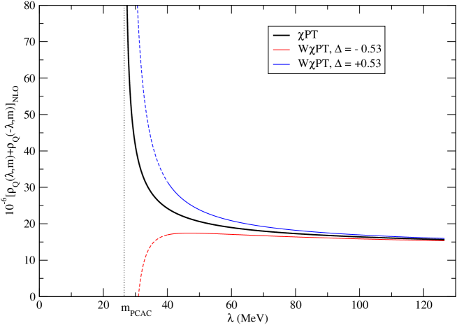
Figure 1: The spectral density $[\rho_{Q}(\lambda,m)+\rho_{Q}(-\lambda,m)]_{NLO}$ in the infinite volume. We used the parameters $\Sigma=(275\;{\rm MeV})^{3}$, $m_{\rm PCAC}=26.5$ MeV,$F=90$ MeV, $\bar{L}_{6}=5$, $\mu=139.6$ MeV. The solid black line corresponds to the continuum $\chi$PT prediction, while the red (blue) lines correspond to the lattice W$\chi$PT prediction ($O(a)$-improved) on eq. (IV.2) with $\hat{a}^{2}W^{\prime}_{8}=\pm 5\cdot 10^{6}\;{\rm MeV}^{4}$, corresponding to $\Delta=\mp 0.53$.

IV.3 Finite volume corrections

Finite-volume effects arise at NLO and can be computed by taking into account the corrections to the propagators given in eq. (20). We can write down the spectral density as sum of the infinite volume and finite-volume corrections:

$$\rho_{Q}^{V}(\lambda,m)+\rho_{Q}^{V}(-\lambda,m)=\rho_{Q}(\lambda,m)+\rho_{Q}(-\lambda,m)+\Delta\rho_{Q}^{V}(\lambda,m)+\Delta\rho_{Q}^{V}(-\lambda,m).$$ (53)

The explicit expression for the finite-volume correction $\Delta\rho_{Q}^{V}(\lambda,m)+\Delta\rho_{Q}^{V}(-\lambda,m)$ is given in App. C, eq. (C.2). By integrating over $\lambda$ we obtain the corresponding finite-volume corrections for the integrated density

$$N^{V}(\Lambda_{1},\Lambda_{2},m)=N(\Lambda_{1},\Lambda_{2},m)+\Delta N^{V}(\Lambda_{1},\Lambda_{2},m).$$ (54)

In eq. (C.2) we give the formula for $\Delta N^{V}(\Lambda_{1},\Lambda_{2},m)$ for the particular case $\Lambda_{1}=m$.

We stress that in our power counting finite-volume effects are insensitive to lattice artefacts at NLO, and these results are the one of the continuum theory already obtained in Giusti and Luscher (2009). In fig. 2 we show the relative correction $\Delta N^{V}(m,\Lambda,m)_{NLO}/N(m,\Lambda,m)_{NLO}$ as a function of $\Lambda$, for two different volumes with $T=3.84$ fm and $L=1.92$ (red dashed curve) and $L=2.56$ fm (black solid curve).
Notice that the finite-volume correction $N^{V}(\Lambda_{1},\Lambda_{2},m)$ diverges at the threshold ($\Lambda_{1}=\Lambda_{2}=m$): this could be interpreted as a signal that, even if the quark mass is in the $p$-regime, another scale comes into play in this problem, namely $\sqrt{\lambda^{2}-m^{2}}$, and it needs to be treated with a different power counting when approaching the threshold at finite volume. Since in the $\epsilon$-expansion of the chiral theory divergences naturally appear when taking the chiral limit at finite volume, this might be the correct power counting to adopt for this additional scale when $\sqrt{\lambda^{2}-m^{2}}\Sigma V\sim 1$. Having said that, for $L\gtrsim 2.0$ fm and sufficiently far from the threshold, finite-volume corrections amount to few percents.

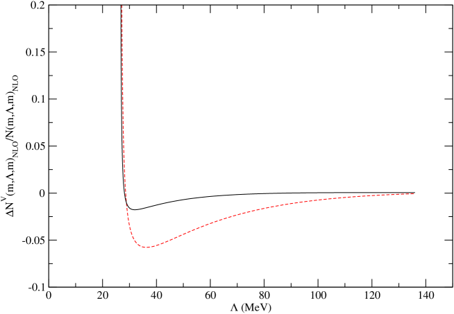
Figure 2: The finite-size effects for the (continuum) integrated spectral density, $\Delta N^{V}(m,\Lambda,m)_{NLO}/N(m,\Lambda,m)_{NLO}$ as a function of $\Lambda$. We used the parameters $\Sigma=(275\;{\rm MeV})^{3}$, $m=m_{\rm PCAC}=26.5$ MeV, $F=90$ MeV, $\bar{L}_{6}=5$, $\mu=139.6$ MeV. The black solid line corresponds to $L=2.56$ fm, $T=3.84$ fm, while the red dashed line corresponds to $L=1.92$ fm, $T=3.84$ fm.

V Discussion of the results and conclusions

The important results of this paper are the expression of the spectral density eq. (IV.2) and its integrated form (C.1). They are both obtained in the $p$-regime of W$\chi$PT at NLO. Eq. (IV.2) shows that the spectral density, when computed on a lattice with Wilson fermions, is modified in two aspects with respect to the NLO continuum formula (see for example refs. Damgaard et al. (1999); Giusti and Luscher (2009) or simply set all the $W$s in eq. (IV.2) to zero). The lattice artefacts modify the behaviour of the spectral density near the threshold, i.e. the term proportional to $\tilde{\Delta}$ in (IV.2), and and its absolute normalisation, i.e. the term proportional to $W_{6}$ in (IV.2). The absolute normalisation correction proportional to $W_{6}$ vanishes if the theory is non-perturbatively O($a$)-improved. If the theory is not improved, beside the term proportional to $W_{6}$, the correction to the normalisation contains in principle an additional O($a$) term stemming from the renormalisation constant $Z_{P}$. We prefer to omit in our final formula (IV.2) this term because it strictly depends on the way $Z_{P}$ is computed and only in very few cases we can have a suitable representation in W$\chi$PT Aoki et al. (2009). We stress nevertheless that when analysing the spectral density computed in the unimproved theory using eq. (IV.2) the O($a$) cutoff effects of $Z_{P}$ have to be taken into account in some way.

More interestingly the cutoff effects modify, the $\lambda$ and $m$ dependence of the continuum formula. These corrections, expressed in terms of the PCAC mass (see eqs. (50-52)), depends on the following LECs: $W_{8}$, $W_{10}$ and $W_{8}^{\prime}$. The modifications induced by cutoff effects to the continuum formula are plotted in fig. 1. To simplify the discussion we have chosen a lattice setup where the theory has been non-perturbatively improved, thus we set all the O($a$) LECs $W_{6}=W_{8}=W_{10}=0$. With the black curve we plot the $\lambda$ dependence of the spectral density in the continuum as given by NLO $\chi$PT Damgaard et al. (1999); Giusti and Luscher (2009) at given values for $m$, $\Sigma$ and $F$ (see the caption of the plot). In the same plot we also show the modifications to the continuum formula induced by W$\chi$PT at NLO. The first observation we make is that the way the spectral density depends on $\lambda$, close to the threshold, is rather different from the continuum formula. The second observation we make is that the W$\chi$PT formula has a rather different behaviour depending on the sign of $W_{8}^{\prime}$, especially close to the threshold. If $\Delta>0$ when $\lambda\rightarrow m_{\rm PCAC}$ the W$\chi$PT formula has a non-integrable singularity, while the continuum formula has an integrable singularity. If $\Delta<0$ the spectral density goes to zero for a value of $\lambda>m_{\rm PCAC}$. These behaviours are shown in fig. 1. This $\lambda$ dependence of the spectral density near the threshold is totally dominated by the lattice NLO corrections induced by the vacuum realignment, indicating that our expansion cannot be trusted for too small $\lambda$. Our power counting breaks down near the threshold: more specifically, it is valid only when $\sqrt{\lambda^{2}-m^{2}}\sim a\Lambda_{\rm QCD}^{2}$, i.e. when the scale $\sqrt{\lambda^{2}-m^{2}}$ obeys a GSM power counting. By moving towards the threshold at finite lattice spacing one enters in the region where $\sqrt{\lambda^{2}-m^{2}}\sim a^{2}\Lambda_{\rm QCD}^{3}$ (Aoki regime), and lattice spacing corrections can not be treated in a perturbative way as it is done in this work. In fig. 1 we draw dashed line where we assume our formula for the spectral density to break down. The minimal $\lambda\simeq 40$ MeV is just an estimate obtained fitting the available numerical data, as we will discuss futher on. It seems a reasonable estimate given the fact that for $\lambda\simeq 40$ MeV the relative lattice spacing NLO corrections are still sufficiently small. Of course this is just an estimate based on the value of $\Delta$ we input, i.e. from the size of the lattice artefacts. Only a thorough analysis of the numerical data can determine the value of $\Delta$, thus the range of validity of our results.

Thus we can try to use our formula (C.1) to fit the available numerical data and see if we obtain reasonable estimates of $\Sigma$ and $\Delta$. To compare our formula with the available numerical data from ref. Giusti and Luscher (2009) we decided to integrate the spectral density from $\lambda=\Lambda_{1}$ and $\lambda=\Lambda_{2}$, taking $\Lambda_{1}=40$ MeV, in order to avoid the small $\lambda$ region where the lattice corrections to the $\chi$PT formula dominate. In order to compare with the results of Giusti and Luscher (2009) we use the mode number defined as $\nu(\Lambda_{1},\Lambda_{2},m)=VN(\Lambda_{1},\Lambda_{2},m)$ and we subtract the value $\nu(0,\Lambda_{1},m)$ from the numerical data.

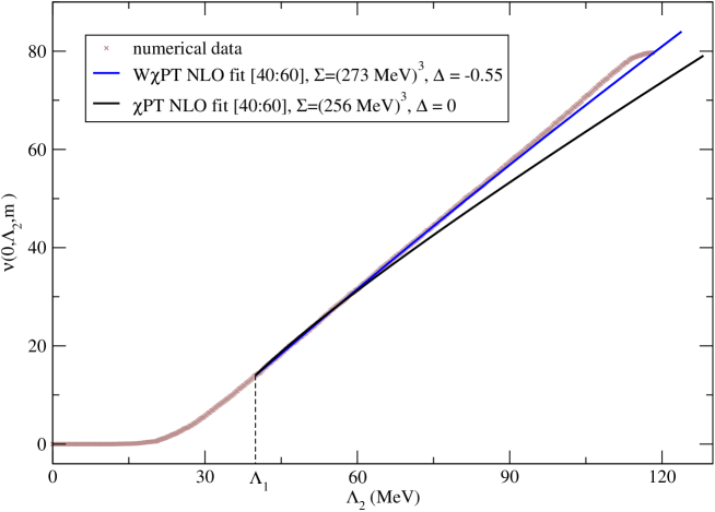
Figure 3: Comparison of the numerical data (red curve) for the mode number $\nu(0,\Lambda_{2},m)$ and the NLO fit results using continuum $\chi$PT (black curve) and W$\chi$PT (blue curve). The fits are obtained using the following parameters: $\Lambda_{1}=40$ MeV $\mu=139.6$ MeV, $F=90$ MeV, $\bar{L}_{6}=5$ and $m_{\rm PCAC}=26.5$ MeV. The fit range is $\Lambda_{2}\in\left[40:60\right]$ MeV.

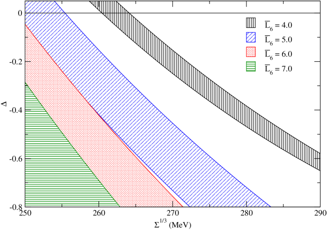
Figure 4: Parameter space of the results obtained fitting the numerical data of ref. Giusti and Luscher (2009) using eq. (C.1). See the main text for details on the fit performed. Only results where a reasonable fit is obtained are showed.

In fig. 3 we show a typical fit of the numerical data of ref. Giusti and Luscher (2009) using the infinite volume formulæ of continuum $\chi$PT and W$\chi$PT in the range $\Lambda_{2}\in\left[40:60\right]$ MeV. The numerical data are obtained at a value of the renormalised PCAC mass $m_{\rm R}\simeq 26$ MeV.
We have performed fits using the both the NLO formulæ of $\chi$PT and W$\chi$PT. With the continuum $\chi$PT formula we have fit $\Sigma$ and fixed the following parameters: $\mu=139.6$ MeV, $F=80,90$ MeV, $\bar{L}_{6}=3,4,\ldots,7$ and $m_{\rm PCAC}=26.5$ MeV. With the W$\chi$PT formula we have set all the O($a$) LECs $W_{6}=W_{8}=W_{10}=0$ because the numerical data are non-perturbatively O($a$)-improved. Additionally we have fixed the value of $\Sigma^{1/3}$ within the range $250-300$ MeV and we have fit $\Delta$. We have performed fits with several forms for the W$\chi$PT formula, all differing by NNLO terms. We have observed that the best fits are obtained with eq. (C.1). In order to decide on the ’best fits’ we have selected the fit results that gives small values of the squared differences between the input data points and the theoretical formula evaluated at the same points.

A summary of the fit results, satisfying our criterion is given in fig. 4. The plot shows the parameter space of the fit results in the $\Delta$, $\Sigma^{1/3}$ plane. Each coloured band represents a fixed value of $\bar{L}_{6}$ and the lower and upper borders of each band represent respectively $F=80$ MeV and $F=90$ MeV. The two most important observations are that reasonable fits are obtained only for $4\lesssim\bar{L}_{6}\lesssim 7$ and for almost the whole parameter space we obtain a negative value of $\Delta$. Our best fit result shown in fig. 3 gives $\Delta=-0.55$ with a value of $\Sigma^{1/3}=273$ MeV, which is in the right ballpark. We will come back to the consequences of this result at the end of this section.
We remark that while the fit results obtained using the continuum NLO formula are not disastrous always a better agreement is found using our W$\chi$PT result.
The W$\chi$PT formula is able to describe well the numerical data also in a larger $\Lambda_{2}$ range, i.e. $\left[40:100\right]$ MeV, with reasonable values of the chiral condensate.
Even if our analysis is rather qualitative and more numerical data are needed, we can try to draw some conclusions. W$\chi$PT describes the numerical data better than continuum $\chi$PT in the range of applicability of our results, i.e. sufficiently away from the threshold, but we cannot exclude that adding NNLO terms in the continuum formula would improve the quality of the fits.

Our fit results seem to prefer a negative value for $\Delta$ implying a positive value for $W_{8}^{\prime}$. In the literature, the LECs $W^{\prime}_{6}$ and $W^{\prime}_{8}$ are often found combined as Aoki and Bär (2004)

$$\hat{a}^{2}\left(W^{\prime}_{6}+\frac{W^{\prime}_{8}}{2}\right)\equiv-\frac{F^{2}c_{2}a^{2}}{16},$$ (55)

which is the combination appearing in quantities computed in full $N_{f}=2$ W$\chi$PT. The chiral phase diagram for Wilson-type fermions depends on the LEC $c_{2}$ (55) and in particular two scenarios can take place depending on its sign. In our case only one of the two LECs appears in the discretisation correction to the spectral density. For large number of colours $N_{c}$, one finds $W_{6}^{\prime}/W_{8}^{\prime}\sim 1/N_{c}$ Sharpe (2006), indicating that $W_{8}^{\prime}$ is the dominant contribution in the coefficient $c_{2}$. This implies that independently on the sign of $W_{6}^{\prime}$ a positive value for $W_{8}^{\prime}$ would suggest a negative value for $c_{2}$. Assuming for instance $W^{\prime}_{6}=W^{\prime}_{8}/3$, then the results we obtain from the fit $\Delta=-0.55$ imply that $\hat{a}^{2}W^{\prime}_{8}=5.4\cdot 10^{6}\;{\rm MeV}^{4}$ which for $a=0.08$ fm would correspond to $c_{2}\simeq-(473\;{\rm MeV})^{4}$. It would be interesting to extend the numerical data in order to establish more accurately the sign of and the absolute value of $W_{8}^{\prime}$. This will give us valuable informations on the behaviour of the spectrum of the Hermitean Wilson operator and a hint on the scenario for the chiral phase diagram that takes place with clover fermions and Wilson gauge action.

We close this section by stressing again an important remark. Our results seem to indicate that apart from the quark mass, the lattice spacing and the lattice size, there is an additional scale entering in this problem, namely the eigenvalues of the massless Dirac operator. In particular, after the analytic continuation of eq. (9) the mass $\sqrt{m^{2}+\mu_{v}^{2}}$ becomes $\sqrt{\lambda^{2}-m^{2}}$, which parametrizes the “distance” from the threshold of the spectral density. Even if we assume, as it is done in this work, that all masses are in the $p-$regime the value of this additional scale can be arbitrarily small. In order to get meaningful results we have to implicitly assume that this parameter obeys the same power counting as the quark masses with respect to the lattice spacing $a$ and the lattice size $L$. While this fact seems trivial at this stage, it is not totally obvious to infer it from the partially quenched initial setup, where valence quarks are introduced as probes to obtain the spectral density. This implies that, at fixed $a$ and $L$, our results will not be valid in the vicinity of the threshold, since from one side the $p$-regime expansion will fail, and from the other side the GSM counting will not be valid anymore, because close to the threshold, as we have discussed before, the NLO corrections induced by the finite lattice spacing dominate the LO result.

We stress that these two effects are decoupled: close to the threshold, there is a scale which in continuum $\chi$PT at finite volume needs to be treated with the $\epsilon$-expansion, and which in W$\chi$PT in infinite volume needs to be treated with the Aoki power counting. The way the two effects combine close to threshold is a not trivial issue and it deserves further investigations.

We conclude that our formula is a useful tool, combined with numerical data, to understand the behaviour of the spectral density of the Hermitean Wilson operator. We also consider this work a necessary and important step towards a complete theoretical understanding of the behaviour close to the threshold of the spectral density of the Hermitean Wilson operator.

VI Acknowledgments

We are indebted to Leonardo Giusti for the access to some crucial private notes on the graded-group method for partially quenched Chiral Effective Theory and for useful discussions. We thank Steve Sharpe and Leonardo Giusti for a critical reading of the manuscript and for precious comments, as well as Martin Lüscher for advices and suggestions and for providing numerical data for the spectral density of the Wilson Dirac operator.

Appendix A SU($m|n$) graded group: conventions and properties

In this Appendix we collect conventions and properties related to SU($m|n$) Cornwell (1989); Giusti (2008) which are relevant for the partially quenched Chiral Effective Theory in the graded-group formulation.

A.1 Supermatrices

For $n,m$ positive integers, a square even supermatrix is defined as a $(m+n)\times(m+n)$ matrix with the structure

$$U=\left(\begin{array}[]{ll}A_{m\times m}&B_{n\times m}\\ C_{m\times n}&D_{n\times n}.\end{array}\right),$$ (56)

where $A$ and $D$ have elements in the even subspace of the Grassmann algebra, while $B$ and $C$ have elements belonging to the odd subspace of the Grassmann algebra (see Cornwell (1989) for definitions and properties of the Grassmann algebras). We define the supertrace of a supermatrix

$${\rm Str}(U)\equiv{\rm Tr}(A)-{\rm Tr}(D),$$ (57)

and the superdeterminant of an invertible supermatrix as

$${\rm Sdet}(U)\equiv{\rm Det}(A-BD^{-1}C)/{\rm Det}(D).$$ (58)

A.2 Superalbegras

We now consider a square $(m+n)\times(m+n)$ matrix with complex entries and the structure

$$M=\left(\begin{array}[]{ll}A_{m\times m}&B_{n\times m}\\ C_{m\times n}&D_{n\times n}.\end{array}\right).$$ (59)

$M$ is said to be even if $B=C=0$, whereas it is odd if $A=D=0$. The degree or parity of $M$ is defined to be

$${\rm deg}\;M=\left\{\begin{array}[]{ll}0&{\rm if}\;M\;{\rm is\;even}\\ 1&{\rm if}\;M\;{\rm is\;odd}\end{array}\right.$$ (60)

One can show that set of all complex linear combinations of these matrices form an associative superalgebra. The supertrace can be defined analogously as in the case of supermatrices,

$${\rm Str}(M)\equiv{\rm Tr}(A)-{\rm Tr}(D).$$ (61)

A.3 Lie supergroups and superalgebras

The Lie Supergroup SU($m|n$) is the set of $(m+n)\times(m+n)$ even supermatrices $U$ satisfying the conditions

$$U^{\dagger}U=1,\;\;\;\;{\rm Sdet}(U)=1.$$ (62)

By parametrizing $U$ as

$$U\equiv e^{i\phi},$$ (63)

these conditions convert into

$$\phi=\phi^{\dagger},\;\;\;\;{\rm Str}(\phi)=0.$$ (64)

The Lie superalgebra associated to SU($m|n$) can be constructed by supplementing the associative superalgebra of $(m+n)\times(m+n)$ complex matrices defined in the previous subsection with the generalised commutators

$$[M,N]=MN-(-1)^{({\rm deg}\;M)({\rm deg}\;N)}NM,$$ (65)

and by requiring the conditions

$$M=M^{\dagger},\;\;\;\;{\rm Str}(M)=0.$$ (66)

A basis for the Lie superalgebra of SU($m|n$) can be chosen to be a set of Hermitian matrices $T^{a}=(T^{a})^{\dagger}$ $(a=1,\ldots,(m+n)^{2}-1)$, with a definite parity

$${\rm deg}(a)\equiv{\rm deg}T^{a},$$ (67)

and zero supertrace

$${\rm Str}(T)^{a}=0.$$ (68)

The normalisation is given by

$${\rm Str}(T^{a}T^{b})=\frac{g^{ab}}{2},$$ (69)

where

$$g^{ab}=\left(\begin{array}[]{lllllllll}1&&&&&&&&\\ &\ddots&&&&&&&\\ &&1&&&&&&\\ &&&-\tau^{2}&&&&&\\ &&&&\ddots&&&&\\ &&&&&-\tau^{2}&&&\\ &&&&&&-1&&\\ &&&&&&&\ddots&\\ &&&&&&&&-1\end{array}\right)\begin{array}[]{ll}\Bigg{\}}&1,\ldots,m^{2}-1\\ &\\ \Bigg{\}}&m^{2},\ldots,m^{2}+2mn-1\\ &\\ \Bigg{\}}&m^{2}+2mn,\ldots,(m+n)^{2}-1,\end{array}$$ (70)

with $g^{ab}=(-1)^{{\rm deg}(a){\rm deg}(b)}g^{ba}$. The elements from $m^{2}$ to $m^{2}+2mn-1$ are odd matrices, while the remaining ones are even.

In this work we consider the particular case of SU(4$|$2). With our conventions, $T^{1},\ldots,T^{15}$ are the (even) generators of the SU(4) subgroup that includes sea and valence quarks, $T^{32},\ldots,T^{34}$ (even) are associated with the SU(2) ghost sector, $T^{16},\ldots,T^{31}$ (odd) mix the ghosts and the quarks, and finally $T^{35}$ (even) is a diagonal matrix with components in both quark and ghost sectors.

For the computation of the propagator it is convenient to introduce the tensors

$$k^{ab} = \left(\frac{1}{\sqrt{3}}g^{a14}+\frac{1}{\sqrt{6}}g^{a15}-\frac{1}{\sqrt{2}}g^{a35}\right)\left(\frac{1}{\sqrt{3}}g^{b14}+\frac{1}{\sqrt{6}}g^{b15}-\frac{1}{\sqrt{2}}g^{b35}\right),$$ (71)

$$h^{ab} = \left(\frac{1}{\sqrt{3}}g^{a14}+\frac{1}{\sqrt{6}}g^{a15}+\frac{1}{\sqrt{2}}g^{a35}\right)\left(\frac{1}{\sqrt{3}}g^{b14}+\frac{1}{\sqrt{6}}g^{b15}+\frac{1}{\sqrt{2}}g^{b35}\right)$$ (72)

which satisfy

$$\sum_{c=1}^{35}h^{ac}k^{cb}=0.$$ (73)

Appendix B The spectral density in W$\chi$PT with the replica method

In this appendix we present the same calculation done in sec. IV applying the replica method Damgaard and Splittorff (2000) in alternative to the graded group method. We consider a partially quenched theory with $N_{s}$ sea quarks of mass $m_{s}$ and $N_{v}$ quenched valence quarks of mass $m_{v}$. For simplicity we set the volume to infinity; finite-volume corrections can be computed in a standard procedure, like explained in sec. IV.3. The replica method consists in enlarging the valence sector to $k$ replica of $N_{v}$ valence quarks. The full symmetry group at zero quark mass is therefore SU$(N_{s}+N_{r})_{L}$$\times$SU$(N_{s}+N_{r})_{R}$, with $N_{r}=kN_{v}$, and the generating functional at the quark level is given by

$$Z_{PQ,replica}(J)=\int[dA_{\mu}]{\rm Det}(D+m_{v}+J)^{N_{v}}{\rm Det}(D+m_{v})^{N_{r}-N_{v}}{\rm Det}(D+m_{s})^{N_{s}}e^{-S_{g}(A_{\mu})},$$ (74)

where we have introduced source terms $J$. In the limit $N_{r}=0$ one reproduces the generating functional in the graded group method Bernard and Golterman (1992, 1994)

$$Z_{PQ,graded}(J)=\int[dA_{\mu}]\frac{{\rm Det}(D+m_{v}+J)^{N_{v}}}{{\rm Det}(D+m_{v})^{N_{v}}}{\rm Det}(D+m_{s})^{N_{s}}e^{-S_{g}(A_{\mu})},$$ (75)

which is obtained in a SU$(N_{s}+N_{v}|N_{v})_{L}$$\times$SU$(N_{s}+N_{v}|N_{v})_{R}$ theory, where internal valence quark loops are cancelled by introducing quarks with the wrong statistics (ghosts). This equivalence is translated into the chiral effective theory and has been verified at the perturbative level Damgaard and Splittorff (2000). In this appendix we explicitly show how this equivalence is realised for the computation of the spectral density starting from the partially quenched pseudoscalar density.

For our specific computation we consider the case $N_{s}=2$, with a doublet of twisted valence quarks. The chiral Lagrangian is the same as in eq. (16), with the “Supertrace” replaced by the conventional trace over the group SU$(N_{s}+N_{r})$. The mass matrix has the form

$$\mathcal{M}={\rm diag}(\underbrace{m}_{2\times 2\;{\rm sea}},\underbrace{\underbrace{m+i\mu_{v}\tau^{3}}_{N_{v}=2},\ldots,m+i\mu_{v}\tau^{3}}_{N_{r}=kN_{v}}).$$ (76)

The pseudo Nambu-Goldstone fields are parametrised by

$$U(x)=u_{V}e^{2i\xi(x)/F}u_{V},\;\;\;\;\xi=\sum_{a}\xi^{a}T^{a},$$ (77)

where now $T^{a},a=1,\ldots,(2+N_{r})^{2}-1$ are the generators of SU$(2+N_{r})$, with the normalisation convention

$${\rm Tr}(T^{a}T^{b})=\frac{\delta^{ab}}{2},$$ (78)

while $u_{V}$ represents the ground state of the theory. By minimising the LO potential we obtain

$$u_{V}={\rm diag}(\underbrace{1}_{2\times 2\;{\rm sea}},\underbrace{e^{i\tau^{3}\omega_{0}/2}}_{N_{r}}),$$ (79)

with the definitions already given in eq. (15)

$$\sin\omega_{0}=\frac{\mu_{v}}{m_{P}},\;\;\;\cos\omega_{0}=\frac{m}{m_{P}},\;\;\;\;m_{P}=\sqrt{m^{2}+\mu_{v}^{2}}.$$ (80)

In this framework it is convenient to write down the pseudo Nambu-Goldstone propagator in explicit components

$$\langle\xi_{ca}(x)\xi_{db}(y)\rangle=\frac{1}{2}\left[\delta_{cb}\delta_{da}G^{1}(x-y,M_{ab}^{2})-\delta_{ca}\delta_{db}E(x-y,M_{aa}^{2},M_{cc}^{2})\right],$$ (81)

with $a,b,c,d=1,\ldots,(2+N_{r})$. The infinite-volume scalar propagator is defined in eq. (21), while

$$E(x-y,M_{aa}^{2},M_{cc}^{2}) \equiv \frac{1}{(2\pi)^{4}}\int d^{4}p\frac{e^{ipx}}{(p^{2}+M_{aa}^{2})(p^{2}+M_{cc}^{2})F(p)},$$ (82)

$$F(p) \equiv \frac{2}{p^{2}+M_{ss}^{2}}+\frac{N_{v}}{p^{2}+M_{vv}^{2}},$$ (83)

with

$$M_{ab}^{2}=B(m_{a}+m_{b})=\left\{\begin{array}[]{ll}M_{ss}^{2}=2mB&{\rm if}\;\;a,b=1,2\\ M_{vv}^{2}=2m_{P}B&{\rm if}\;\;a,b=3,\ldots,N_{r}\\ M_{sv}^{2}=(m+m_{P})B&{\rm if}\;\;a(b)=1,2;b(a)=3,\ldots,N_{r}.\end{array}\right.$$ (84)

The observable we have to consider in order to extract the spectral density is the expectation value of the pseudoscalar density defined in eq. (8). The pseudoscalar density can be obtained by taking the functional derivative of the action with respect to appropriate sources, which are introduced by the following procedure:

$$\mathcal{M}\rightarrow\mathcal{M}+\hat{\tau}^{3}p^{3}(x),\;\;\;\;\mathcal{M}^{\dagger}\rightarrow\mathcal{M}^{\dagger}-\hat{\tau}^{3}p^{3}(x),$$ (85)

where $\hat{\tau}^{3}$ has non-zero elements only in one of the replica of the valence sector

$$\hat{\tau}^{3}={\rm diag}(\underbrace{0}_{2\times 2\;{\rm sea}},\underbrace{\underbrace{\tau^{3}}_{N_{v}=2},0}_{N_{r}}).$$ (86)

At LO we obtain the (continuum) expectation value

$$\langle\mathcal{P}^{3}\rangle_{LO}=2i\Sigma\sin\omega_{0}.$$ (87)

This result is independent on $N_{r}$, and coincide with the one obtained with the graded group method, eq. (28). At $O(p^{2})$ we obtain

$$\langle\mathcal{P}^{3}\rangle_{NLO} = 2i\Sigma\sin(\omega_{0})\Bigg{\{}1+\delta\cot\omega_{0}-\frac{1}{F^{2}}\Bigg{[}2G^{1}(0,M^{2}_{sv})+N_{r}G^{1}(0,M^{2}_{vv})$$

$$- E(0,M^{2}_{vv},M^{2}_{vv})-16L_{6}(2M^{2}_{ss}+N_{r}M^{2}_{vv})-4M^{2}_{vv}(H_{2}+2L_{8})$$

$$- 8\hat{a}\left(W_{6}\left(2+N_{r}\cos\omega_{0}\right)+W_{8}\cos\omega_{0}\right)\Bigg{]}\Bigg{\}}$$

The shift $\delta$ is the $O(p^{2})$ correction to the ground state angle $\omega_{0}$ that must be computed by minimising the NLO potential. Unlike the graded group case discussed in sec. IV.1, with the replica method the minimisation is trivial, since the fields belong to the conventional SU$(N_{s}+N_{r})$ group. By taking only the linear term in $N_{r}$ we get

$$\delta=-\frac{16\hat{a}\sin\omega_{0}}{F^{2}}\left\{\left(W_{6}\cos\omega_{0}+\frac{W_{8}}{2}\right)+\frac{2\hat{a}}{M^{2}_{vv}}\left(W_{6}^{\prime}+\frac{W_{8}^{\prime}}{2}\cos\omega_{0}\right)\right\},$$ (89)

which coincides with the shift calculated with the graded groups in sec. IV.1, eq. (44). The final result in the limit $N_{r}\rightarrow 0$ for the partially quenched pseudoscalar density at NLO is then

$$\langle\mathcal{P}^{3}\rangle_{NLO} = 2i\Sigma\sin\omega_{0}\Bigg{\{}1+\delta\cot\omega_{0}+\frac{1}{F^{2}}\Bigg{[}\frac{1}{2}G^{1}(0,M^{2}_{vv})-2G^{1}(0,M^{2}_{sv})+32L_{6}M^{2}_{ss}$$

$$- \frac{1}{2}(M^{2}_{vv}-M^{2}_{ss})G^{2}(0,M^{2}_{vv})+4M^{2}_{vv}(H_{2}+2L_{8})+8\hat{a}\left(2W_{6}+W_{8}\cos\omega_{0}\right)\Bigg{]}\Bigg{\}},$$

where we have used

$$E(0,M^{2}_{vv},M^{2}_{vv})|_{N_{r}\rightarrow 0}=\frac{1}{2}G^{1}(0,M^{2}_{vv})-\frac{1}{2}(M^{2}_{vv}-M^{2}_{ss})G^{2}(0,M^{2}_{vv}).$$ (91)

This result for the pseudoscalar density is fully equivalent to the one obtained with the graded groups, eq. (IV), as expected.

Appendix C Some explicit formulae

In this Appendix we collect some explicit formulae which we omitted in the main text for clarity reasons.

C.1 Integrated spectral density at NLO

We report the integrated spectral density computed at NLO in W$\chi$PT. Starting from the result presented in eq. (IV.2) for the spectral density, we obtain:

$$N(\Lambda_{1},\Lambda_{2},m)_{NLO} \equiv \int_{\Lambda_{1}}^{\Lambda_{2}}d\lambda\;[\rho_{Q}(\lambda,m)+\rho_{Q}(-\lambda,m)]_{NLO}=$$

$$= \frac{2\Sigma}{\pi}\Bigg{\{}\left(\sqrt{\Lambda_{2}^{2}-m^{2}}-\sqrt{\Lambda_{1}^{2}-m^{2}}\right)\left(1+\frac{16\hat{a}}{F^{2}}W_{6}\right)$$

$$- \tilde{\Delta}m^{2}\left(\frac{1}{\sqrt{\Lambda_{2}^{2}-m^{2}}}-\frac{1}{\sqrt{\Lambda_{1}^{2}-m^{2}}}\right)$$

$$+ \frac{\Sigma}{(4\pi)^{2}F^{4}}\Bigg{[}-\frac{\pi}{2}(\Lambda_{2}^{2}-\Lambda_{1}^{2})+m(1+3\bar{L}_{6})\left(\sqrt{\Lambda_{2}^{2}-m^{2}}-\sqrt{\Lambda_{1}^{2}-m^{2}}\right)$$

$$+ (\Lambda_{2}^{2}-2m^{2})\arctan\left(\frac{\sqrt{\Lambda_{2}^{2}-m^{2}}}{m}\right)-(\Lambda_{1}^{2}-2m^{2})\arctan\left(\frac{\sqrt{\Lambda_{1}^{2}-m^{2}}}{m}\right)$$

$$- m\sqrt{\Lambda_{2}^{2}-m^{2}}\left(2\log\left(\frac{\Sigma\Lambda_{2}}{F^{2}\mu^{2}}\right)+\log\left(\frac{2\Sigma\sqrt{\Lambda_{2}^{2}-m^{2}}}{F^{2}\mu^{2}}\right)\right)$$

$$+ m\sqrt{\Lambda_{1}^{2}-m^{2}}\left(2\log\left(\frac{\Sigma\Lambda_{1}}{F^{2}\mu^{2}}\right)+\log\left(\frac{2\Sigma\sqrt{\Lambda_{1}^{2}-m^{2}}}{F^{2}\mu^{2}}\right)\right)\Bigg{]}\Bigg{\}},$$

where $\tilde{\Delta}$ is given in eq. (47).

C.2 Finite volume corrections

In this section we give explicit expressions for the finite volume corrections defined in eqs. (53),(54). It is convenient to represent the finite-volume propagator $g_{r}(M^{2})$ Hasenfratz and Leutwyler (1990) defined in eq. (20) as sum over modified Bessel functions $K_{\nu}$:

$$g_{r}(M^{2})=\frac{1}{\Gamma(r)(4\pi)^{2}}\sum_{\{n1,n2,n3,n4\}\neq 0}F_{r-2}\left(\frac{q_{n}^{2}}{4},M^{2}\right),$$ (93)

with $q_{n}^{2}=\left((n_{1}^{2}+n_{2}^{2}+n_{3}^{2})L^{2}+n_{4}^{2}T^{2}\right)$ and

$$F_{\nu}(a,z)=2\left(\frac{a}{z}\right)^{\nu/2}K_{\nu}(2\sqrt{az}).$$ (94)

Using this representation one obtains the finite-volume correction to the spectral density

$$[\Delta\rho_{Q}^{V}(\lambda,m)+\Delta\rho_{Q}^{V}(-\lambda,m)]_{NLO} = \frac{\Sigma}{\pi}\frac{\Sigma}{F^{4}(4\pi)^{2}}\frac{2\lambda}{\sqrt{\lambda^{2}-m^{2}}}\sum_{\{n1,n2,n3,n4\}\neq 0}$$

$$\Bigg{\{}{\rm Re}\left[F_{-1}\left(\frac{\Sigma q_{n}^{2}}{2F^{2}},i\sqrt{\lambda^{2}-m^{2}}\right)\right]$$

$$- 2{\rm Re}\left[F_{-1}\left(\frac{\Sigma q_{n}^{2}}{4F^{2}},m+i\sqrt{\lambda^{2}-m^{2}}\right)\right]$$

$$+ \sqrt{\lambda^{2}-m^{2}}{\rm Im}\left[F_{0}\left(\frac{\Sigma q_{n}^{2}}{2F^{2}},i\sqrt{\lambda^{2}-m^{2}}\right)\right]$$

$$+ m{\rm Re}\left[F_{0}\left(\frac{\Sigma q_{n}^{2}}{2F^{2}},i\sqrt{\lambda^{2}-m^{2}}\right)\right]\Bigg{\}}.$$

The corresponding correction for the integrated spectral density $N^{V}(\Lambda_{1},\Lambda_{2},m)_{NLO}$ for $\Lambda_{1}=m$ is given by

$$\Delta N^{V}(m,\Lambda_{2},m)_{NLO} = \int_{m}^{\Lambda_{2}}[\Delta\rho_{Q}^{V}(\lambda,m)+\Delta\rho_{Q}^{V}(-\lambda,m)]_{NLO}d\lambda=\frac{2\Sigma^{2}}{\pi}\frac{\sqrt{\Lambda_{2}^{2}-m^{2}}}{(4\pi)^{2}F^{4}}$$

$$\sum_{\{n1,n2,n3,n4\}\neq 0}\Bigg{\{}\frac{2}{\sqrt{\Lambda_{2}^{2}-m^{2}}}{\rm Im}\left[F_{-2}\left(\frac{\Sigma q_{n}^{2}}{4F^{2}},i\sqrt{\Lambda_{2}^{2}-m^{2}}+m\right)\right]$$

$$- \frac{m}{\sqrt{\Lambda_{2}^{2}-m^{2}}}{\rm Im}\left[F_{-1}\left(\frac{\Sigma q_{n}^{2}}{2F^{2}},i\sqrt{\Lambda_{2}^{2}-m^{2}}\right)\right]$$

$$+ {\rm Re}\left[F_{-1}\left(\frac{\Sigma q_{n}^{2}}{2F^{2}},i\sqrt{\Lambda_{2}^{2}-m^{2}}\right)\right]\Bigg{\}}.$$

References

- Hasenbusch and Jansen (2003) M. Hasenbusch and K. Jansen, Nucl.Phys. B659, 299 (2003), eprint hep-lat/0211042.
- Luscher (2005) M. Luscher, Comput.Phys.Commun. 165, 199 (2005), eprint hep-lat/0409106.
- Urbach et al. (2006) C. Urbach, K. Jansen, A. Shindler, and U. Wenger, Comput. Phys. Commun. 174, 87 (2006), eprint hep-lat/0506011.
- Clark and Kennedy (2007) M. Clark and A. Kennedy, Phys.Rev.Lett. 98, 051601 (2007), eprint hep-lat/0608015.
- Luscher (2007) M. Luscher, JHEP 0707, 081 (2007), eprint arXiv:0706.2298.
- Del Debbio et al. (2006) L. Del Debbio, L. Giusti, M. Luscher, R. Petronzio, and N. Tantalo, JHEP 02, 011 (2006), eprint hep-lat/0512021.
- Giusti and Luscher (2009) L. Giusti and M. Luscher, JHEP 0903, 013 (2009), eprint arXiv:0812.3638.
- Del Debbio et al. (2007) L. Del Debbio, L. Giusti, M. Luscher, R. Petronzio, and N. Tantalo, JHEP 0702, 082 (2007), eprint hep-lat/0701009.
- Sharpe and Singleton (1998) S. R. Sharpe and R. L. Singleton, Phys. Rev. D58, 074501 (1998), eprint hep-lat/9804028.
- Rupak and Shoresh (2002) G. Rupak and N. Shoresh, Phys. Rev. D66, 054503 (2002), eprint hep-lat/0201019.
- Aoki (1984) S. Aoki, Phys. Rev. D30, 2653 (1984).
- Sharpe (2006) S. R. Sharpe, Phys. Rev. D74, 014512 (2006), eprint hep-lat/0606002.
- Damgaard et al. (2010) P. Damgaard, K. Splittorff, and J. Verbaarschot, Phys.Rev.Lett. 105, 162002 (2010), eprint arXiv:1001.2937.
- Akemann et al. (2010) G. Akemann, P. Damgaard, K. Splittorff, and J. Verbaarschot (2010), eprint arXiv:1012.0752.
- Shindler (2009) A. Shindler, Phys. Lett. B672, 82 (2009), eprint arXiv:0812.2251.
- Bär et al. (2009) O. Bär, S. Necco, and S. Schaefer, JHEP 03, 006 (2009), eprint arXiv:0812.2403.
- Bär et al. (2010) O. Bär, S. Necco, and A. Shindler, JHEP 04, 053 (2010), eprint arXiv:1002.1582.
- Banks and Casher (1980) T. Banks and A. Casher, Nucl. Phys. B169, 103 (1980).
- Chandrasekharan (1995) S. Chandrasekharan, Nucl. Phys. Proc. Suppl. 42, 475 (1995), eprint hep-lat/9412070.
- Verbaarschot (1996) J. J. M. Verbaarschot, Phys. Lett. B368, 137 (1996), eprint hep-ph/9509369.
- Osborn et al. (1999) J. C. Osborn, D. Toublan, and J. J. M. Verbaarschot, Nucl. Phys. B540, 317 (1999), eprint hep-th/9806110.
- Symanzik (1983a) K. Symanzik, Nucl. Phys. B226, 187 (1983a).
- Symanzik (1983b) K. Symanzik, Nucl. Phys. B226, 205 (1983b).
- Sharpe and Wu (2004) S. R. Sharpe and J. M. S. Wu, Phys. Rev. D70, 094029 (2004), eprint hep-lat/0407025.
- Sharpe and Wu (2005) S. R. Sharpe and J. M. S. Wu, Phys. Rev. D71, 074501 (2005), eprint hep-lat/0411021.
- Bernard and Golterman (1992) C. W. Bernard and M. F. L. Golterman, Phys. Rev. D46, 853 (1992), eprint hep-lat/9204007.
- Bernard and Golterman (1994) C. W. Bernard and M. F. L. Golterman, Phys. Rev. D49, 486 (1994), eprint hep-lat/9306005.
- Damgaard and Splittorff (2000) P. H. Damgaard and K. Splittorff, Phys. Rev. D62, 054509 (2000), eprint hep-lat/0003017.
- Giusti (2008) L. Giusti, Private notes (2008).
- Hasenfratz and Leutwyler (1990) P. Hasenfratz and H. Leutwyler, Nucl. Phys. B343, 241 (1990).
- Gasser and Leutwyler (1985) J. Gasser and H. Leutwyler, Nucl. Phys. B250, 465 (1985).
- Bär et al. (2004) O. Bär, G. Rupak, and N. Shoresh, Phys. Rev. D70, 034508 (2004), eprint hep-lat/0306021.
- Aoki (2003) S. Aoki, Phys. Rev. D68, 054508 (2003), eprint hep-lat/0306027.
- Sharpe and Shoresh (2001) S. R. Sharpe and N. Shoresh, Phys. Rev. D64, 114510 (2001), eprint hep-lat/0108003.
- Golterman et al. (2005) M. Golterman, S. R. Sharpe, and J. Singleton, Robert L., Phys. Rev. D71, 094503 (2005), eprint hep-lat/0501015.
- Gasser and Leutwyler (1984) J. Gasser and H. Leutwyler, Ann. Phys. 158, 142 (1984).
- Damgaard et al. (1999) P. H. Damgaard, J. C. Osborn, D. Toublan, and J. J. M. Verbaarschot, Nucl. Phys. B547, 305 (1999), eprint hep-th/9811212.
- Aoki et al. (2009) S. Aoki, O. Bär, and S. R. Sharpe, Phys. Rev. D80, 014506 (2009), eprint arXiv:0905.0804.
- Aoki and Bär (2004) S. Aoki and O. Bär, Phys. Rev. D70, 116011 (2004), eprint hep-lat/0409006.
- Farchioni et al. (2005a) F. Farchioni, R. Frezzotti, K. Jansen, I. Montvay, G. Rossi, et al., Eur.Phys.J. C39, 421 (2005a), eprint hep-lat/0406039.
- Farchioni et al. (2005b) F. Farchioni, K. Jansen, I. Montvay, E. Scholz, L. Scorzato, et al., Eur.Phys.J. C42, 73 (2005b), eprint hep-lat/0410031.
- Farchioni et al. (2005c) F. Farchioni, K. Jansen, I. Montvay, E. Scholz, L. Scorzato, et al., Phys.Lett. B624, 324 (2005c), eprint hep-lat/0506025.
- Cornwell (1989) J. Cornwell, Group Theory in Physics. Vol. 3: Supersymmetries and infinite dimensional Algebras (1989).