On the Coupling-Strength Growth
of the Rabi Model
in the Light of SUSYQM

Abstract

We consider the coupling-strength growth of the Rabi model from the point of the view of SUSYQM. We show that the Rabi model takes the supersymmetric system to the spontaneous supersymmetry breaking as its coupling strength $\mathrm{g}$ grows lager from the case $\mathrm{g}=0$ to the case $\mathrm{g}\approx\infty$. We study a kind of chirality quantum phase transition in this process.

1 Introduction

Supersymmetric quantum mechanics (SUSYQM) was initiated by Witten [1], and has been developed by many physicists [2, 3, 4, 5, 6, 7, 8, 9, 10, 11, 12, 13]. In particular, some ground state structures and the spontaneous supersymmetry (SUSY) breaking in SUSYQM have been investigated [4, 8, 9, 13]. We are interested in ground state structure in SUSYQM from another point of view than their preceding studies. We will handle the Rabi model that has the interaction between a $2$-level atom and the light in a cavity. The Rabi model is sometimes called the full Jaynes-Cummings model. That is, its Hamiltonian has full linear coupling of the $2$-level atom and the light without the rotating wave approximation (RWA). The Rabi model has been well studied in quantum optics, and its some inherent properties have been beginning to experimentally observed in cavity quantum electrodynamics (QED) and circuit QED [14, 15, 16, 17, 18, 19, 20]. We take an interest in the physical properties that a qubit of the $2$-level atom coupled with the light makes in SUSYQM. We are conjecturing that the spontaneous SUSY breaking recovers a chirality in the Rabi model.

The interaction between an atom and the light in nature follows the QED. It is governed by the fine-structure constant $\alpha\approx 0.00729735$, belonging to the region over which the perturbation theory is valid. On the other hand, cavity QED handles stronger interaction than the standard QED does [14, 15]. Such a strong interaction is experimentally prepared with the coupling of a two-level atom and a one-mode light (i.e., single-mode laser) in a mirror cavity (i.e., a mirror resonator). Several solid-state analogues of the strong coupling had been foreseen in superconducting systems [16, 17]. In short, we respectively replace the atom, the light, and the mirror resonator in cavity QED by an artificial atom, a microwave, and a microwave resonator on a superconducting circuit. The artificial atom consists of a superconducting circuit based on some Josephson junctions then. This replaced cavity QED is circuit QED, which has been experimentally demonstrated [18, 19]. It is remarkable that circuit QED has been capable of intensifying the coupling strength further than cavity QED has [20].

In this paper we pay our particular attention on the coupling-strength growth of the Rabi model from the point of the view of SUSYQM. We will show that the Rabi model takes SUSY system to the spontaneous SUSY breaking as its coupling strength $\mathrm{g}$ grows lager from the case $\mathrm{g}=0$ to the case $\mathrm{g}\approx\infty$. We will also show that this spontaneous SUSY breaking is caused by the spin-chirality between the two levels of the atom. We are then interested in when and how the spin-chirality works. We will consider a problem similar to Hund’s paradox on the chiral molecules [21, 22], and show a kind of chirality quantum phase transition (CQPT) [23] in the process from the SUSY system to the system with spontaneous SUSY breaking. This makes us expect that we can realize the quantum simulation [24] of some properties of SUSYQM in circuit QED.

2 SUSY and Spontaneous Breaking in Rabi Model

In this section we consider two special cases to find some SUSYQM aspects in the Rabi model.

We denote the annihilation (resp. creation) operator for the one-mode photon by $a$ (resp. $a^{\dagger}$). We use the standard notation for the Pauli matrices as $\sigma_{x}\equiv\bigl{(}\begin{smallmatrix}0&1\\ 1&0\end{smallmatrix}\bigr{)}$, $\sigma_{y}\equiv\bigl{(}\begin{smallmatrix}0&-i\\ i&0\end{smallmatrix}\bigr{)}$, and $\sigma_{z}\equiv\bigl{(}\begin{smallmatrix}1&0\\ 0&-1\end{smallmatrix}\bigr{)}$. We define spin states $|\!\!\uparrow\rangle$ and $|\!\!\downarrow\rangle$ by $|\!\!\uparrow\rangle:=\bigl{(}\begin{smallmatrix}1\\ 0\end{smallmatrix}\bigr{)}$ and $|\!\!\downarrow\rangle:=\bigl{(}\begin{smallmatrix}0\\ 1\end{smallmatrix}\bigr{)}$. We denote by $\mathcal{F}$ the Fock space of the one-mode photon, and by $|n\rangle$ the Fock state with the photon number $n=0,1,2,\cdots$. So, in particular, $|0\rangle$ denotes the Fock vacuum. Every quantum state that we will use in this paper is represented as $|n,\sharp\rangle:=|n\rangle|\sharp\rangle$ for $n=0,1,2,\cdots$ and $\sharp=\uparrow,\downarrow$. Here, we omitted the tensor-notation $\otimes$ from the expression $|n\rangle\otimes|\sharp\rangle$. We will use this omitted notation throughout this paper. Also, we denote by $|\psi,\sharp\rangle$ the state $|\psi\rangle|\sharp\rangle$ for the state $\psi$ in the Fock space $\mathcal{F}$. Let us give the subspace $\mathcal{H}_{\mathrm{even}}$ (resp. $\mathcal{H}_{\mathrm{odd}}$) as the set of all of the states $|\psi,\uparrow\rangle$ (resp. $|\psi,\downarrow\rangle$), where the state $\psi$ runs over the whole Fock space. Then, the state space $\mathcal{H}$ is obviously decomposed as the direct sum of $\mathcal{H}_{\mathrm{even}}$ and $\mathcal{H}_{\mathrm{odd}}$: $\mathcal{H}=\mathcal{H}_{\mathrm{even}}\oplus\mathcal{H}_{\mathrm{odd}}$.

The free Hamiltonian $H_{0}$ of the Rabi model is given by

$$H_{0}:=\frac{\hbar\omega_{\mathrm{a}}}{2}\sigma_{z}+\hbar\omega_{\mathrm{c}}\left(a^{\dagger}a+\frac{1}{2}\right).$$

The constants $\omega_{\mathrm{a}}$ and $\omega_{\mathrm{c}}$ are respectively the (artificial) atom transition frequency and the cavity resonance frequency. Then, the Rabi Hamiltonian $H_{\mathrm{Rabi}}$ is given by

$$H_{\mathrm{Rabi}}:=H_{0}+\hbar\mathrm{g}\left(a+a^{\dagger}\right)\sigma_{x},$$ (1)

where the parameter $\mathrm{g}\geq 0$ stands for the atom-photon coupling constant that represents the coupling strength. The solvability of the Rabi Hamiltonian has been argued by Braak [25], by using Bargmann’s representation [27]. Here, we give a numerical computation of the energies of the Rabi model in the case $\omega:=\omega_{\mathrm{a}}=\omega_{\mathrm{c}}$ in Fig.1.

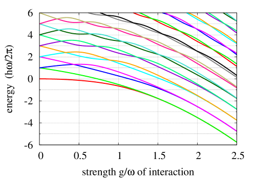
Figure 1: Energy Levels of $H_{\mathrm{Rabi}}$ for $\omega:=\omega_{\mathrm{a}}=\omega_{\mathrm{c}}$. Each color indicates the $n$th level of the energy for $n=0,1,2,\cdots$ from the bottom, where the $0$th level energy means the ground-state energy.

Fig.1 attracts our particular attention to the two special cases, $\mathrm{g}=0$ and $\mathrm{g}\approx\infty$, in the light of SUSYQM. In the case $\mathrm{g}=0$, the ground state is unique, but all the excited states are $2$-fold degenerate. All the eigenenergies line up at an equal interval $\hbar\omega$ then. Meanwhile, in case $\mathrm{g}\approx\infty$, Fig.1 makes us expect that all the states are almost $2$-fold degenerate, and all the eigenenergies are aligned at an almost equal interval $\hbar\omega$. We now investigate these physical situations in detail from the point of the view of SUSYQM for a while. Let us take the two frequencies as $\omega:=\omega_{\mathrm{a}}=\omega_{\mathrm{c}}$ throughout this paper, and then, we denote the free Hamiltonian $H_{0}$ by $H_{\mathrm{SS}}$:

$$H_{\mathrm{SS}}:=\frac{\hbar\omega}{2}\sigma_{z}+\hbar\omega\left(a^{\dagger}a+\frac{1}{2}\right).$$ (2)

We note that it is easy to control the two frequencies $\omega_{\mathrm{a}}$ and $\omega_{\mathrm{c}}$ in circuit QED so that they are equal.

First up, when there is no interaction between the (artificial) atom and the light (i.e., $\mathrm{g}=0$), the Rabi Hamiltonian becomes the free Hamiltonian: $H_{\mathrm{Rabi}}=H_{\mathrm{SS}}$. So, it is the most popular Hamiltonian in SUSYQM: $H_{\mathrm{Rabi}}=(1/2m)\left(p^{2}+W^{2}+\hbar(dW/dx)\sigma_{z}\right)$ with the correspondence, $a=\sqrt{m\omega/2\hbar}\,x+ip/\sqrt{2m\hbar\omega}$ and $a^{\dagger}=\sqrt{m\omega/2\hbar}\,x-ip/\sqrt{2m\hbar\omega}$ for the position operator $x$ and the momentum operator $p$, where the superpotential $W$ is given by $W(x)=m\omega x$. Namely, the system has $N=2$  SUSY. More precisely, the supercharges $Q_{1}$ and $Q_{2}$ defined by $Q_{1}=(1/2\sqrt{m})(W\sigma_{x}-p\sigma_{y})$ and $Q_{2}=(1/2\sqrt{m})(W\sigma_{y}+p\sigma_{x})$ make the relations:

$$\left\{Q_{k},Q_{\ell}\right\}=\delta_{k\ell}H_{\mathrm{Rabi}},$$

$$\left[Q_{k},H_{\mathrm{Rabi}}\right]=0,$$

$$\left\{Q_{k},N_{\mathrm{F}}\right\}=0,$$

for $k,\ell=1,2$, and the grading operator $N_{\mathrm{F}}=\sigma_{z}$ satisfying the conditions, $N_{\mathrm{F}}\psi_{\mathrm{even}}=\psi_{\mathrm{even}}$ for any state $\psi_{\mathrm{even}}\in\mathcal{H}_{\mathrm{even}}$, and $N_{\mathrm{F}}\psi_{\mathrm{odd}}=\,-\psi_{\mathrm{odd}}$ for any state $\psi_{\mathrm{odd}}\in\mathcal{H}_{\mathrm{odd}}$. Here the symbol $\delta_{k\ell}$ is the Kronecker delta. Then, the system has no SUSY breaking. That is, the supersymmetric (SUSY) ground state is $|0,\downarrow\rangle$ and therefore the ground state energy is equal to zero in this case. In addition, for $\mathrm{g}=0$, the ground state of the Rabi Hamiltonian is unique [26], but all of its excited states are $2$-fold degenerate. The two degenerate excited states are interchanged with each other by the SUSY-generating charges $Q^{+}$ and $Q^{-}$ defined by $Q^{+}:=\sqrt{\hbar\omega}\,a\sigma_{+}$ and $Q^{-}:=\sqrt{\hbar\omega}\,a^{\dagger}\sigma_{-}$. Here, $\sigma_{-}$ and $\sigma_{+}$ are the spin annihilation and creation operators defined by $\sigma_{\pm}:=(\sigma_{x}\pm i\sigma_{y})/2$:

$$Q^{-}|n,\downarrow\rangle=Q^{+}|n,\uparrow\rangle=0,$$

$$|n,\uparrow\rangle=\frac{1}{\sqrt{\hbar\omega(n+1)}}Q^{+}|n+1,\downarrow\rangle,$$

$$|n+1,\downarrow\rangle=\frac{1}{\sqrt{\hbar\omega(n+1)}}Q^{-}|n,\uparrow\rangle,$$

for $n=0,1,2,\cdots$. As is well known, of course, we have

$$\left\{Q^{\pm},Q^{\pm}\right\}=0\,\,\,\text{and}\,\,\,H_{\mathrm{Rabi}}=\left\{Q^{+},Q^{-}\right\}.$$

On the other hand, let us take the coupling strength $\mathrm{g}$ large enough now. We can easily expect that the photon part energy,

$$H_{\mathrm{asym}}:=\hbar\omega\left(a^{\dagger}a+\frac{1}{2}\right)+\hbar\mathrm{g}\left(a+a^{\dagger}\right)\sigma_{x},$$

is asymptotically much more dominant than the $2$-level atom energy $\hbar\omega\sigma_{z}/2$. Namely, the atom energy $\hbar\omega\sigma_{z}/2$ works as a very small perturbation for the photon part energy $H_{\mathrm{asym}}$ around $\mathrm{g}\approx\infty$ [28]. We can show this in a mathematically exact way. We define a unitary operator $U_{\mathrm{g}}$ by

$$U_{\mathrm{g}}:=\frac{1}{\sqrt{2}}\begin{pmatrix}V_{-}&-V_{+}\\ V_{-}&V_{+}\end{pmatrix}$$

with the unitary operator $V_{\pm}:=e^{\pm\mathrm{g}(a^{\dagger}-a)/\omega}$. Recall the well-known Bogoliubov transformation:

$$V_{\pm}\left\{\hbar\omega\left(a^{\dagger}a+\frac{1}{2}\right)\pm\hbar\mathrm{g}\left(a+a^{\dagger}\right)\right\}V_{\mp}=\hbar\omega\left(a^{\dagger}a+\frac{1}{2}\right)-\hbar\frac{\mathrm{g}^{2}}{\omega}.$$ (3)

We reach the unitary transformation,

$$U_{\mathrm{g}}^{*}H_{\mathrm{Rabi}}U_{\mathrm{g}}=U_{\mathrm{g}}^{*}H_{\mathrm{asym}}U_{\mathrm{g}}-\,\frac{\hbar\omega}{2}\widetilde{V}_{\mathrm{g}}=\widetilde{H}_{0}-\,\hbar\frac{\mathrm{g}^{2}}{\omega}-\,\frac{\hbar\omega}{2}\widetilde{V}_{\mathrm{g}}$$ (4)

with the asymptotically free Hamiltonian

$$\widetilde{H}_{0}=\begin{pmatrix}\hbar\omega\left(a^{\dagger}a+\frac{1}{2}\right)&0\\ 0&\hbar\omega\left(a^{\dagger}a+\frac{1}{2}\right)\end{pmatrix}$$

and the unitary, self-adjoint interaction

$$\widetilde{V}_{\mathrm{g}}=\begin{pmatrix}0&e^{2\mathrm{g}(a^{\dagger}-a)/\omega}\\ e^{-2\mathrm{g}(a^{\dagger}-a)/\omega}&0\\ \end{pmatrix}.$$

For arbitrary wave functions $\psi=\bigl{(}\begin{smallmatrix}\psi_{1}\\ \psi_{2}\end{smallmatrix}\bigr{)}$ and $\phi=\bigl{(}\begin{smallmatrix}\phi_{1}\\ \phi_{2}\end{smallmatrix}\bigr{)}$, we set $\widetilde{\psi}_{j}:=e^{i\pi a^{\dagger}a/2}\psi_{j}$ and $\widetilde{\phi}_{j}:=e^{i\pi a^{\dagger}a/2}\phi_{j}$. Using the equations, $e^{i\pi a^{\dagger}a/2}ae^{-i\pi a^{\dagger}a/2}=-ia$ and $e^{i\pi a^{\dagger}a/2}a^{\dagger}e^{-i\pi a^{\dagger}a/2}=ia$, we have

$$\langle\psi|\widetilde{V}_{\mathrm{g}}|\phi\rangle =\langle\psi_{1}|e^{2\mathrm{g}(a^{\dagger}-a)/\omega}\phi_{2}\rangle+\langle\psi_{2}|e^{-2\mathrm{g}(a^{\dagger}-a)/\omega}\phi_{1}\rangle$$

$$=\langle\widetilde{\psi}_{1}|e^{i(2\mathrm{g}/\omega)(a^{\dagger}+a)}\widetilde{\phi}_{2}\rangle+\langle\widetilde{\psi}_{2}|e^{-i(2\mathrm{g}/\omega)(a^{\dagger}+a)}\widetilde{\phi}_{1}\rangle.$$

Since we have $a^{\dagger}+a=\sqrt{2m\omega/\hbar}\,x$, we obtain the representation:

$$\langle\psi|\widetilde{V}_{\mathrm{g}}|\phi\rangle=\int dx\widetilde{\psi}_{1}^{*}(x)\widetilde{\phi}_{2}(x)e^{i(2\mathrm{g}\sqrt{2m/\hbar\omega})x}+\int dx\widetilde{\psi}_{2}^{*}(x)\widetilde{\phi}_{1}(x)e^{-i(2\mathrm{g}\sqrt{2m/\hbar\omega})x}.$$

The Riemann-Lebesgue’s theorem tells us the term vanishes as

$$\lim_{\mathrm{g}\to\infty}\langle\psi|\widetilde{V}_{\mathrm{g}}|\phi\rangle=0$$ (5)

in spite of the equation,

$$\langle\psi|\widetilde{V}_{\mathrm{g}}^{*}\widetilde{V}_{\mathrm{g}}|\psi\rangle=\langle\psi|\psi\rangle.$$ (6)

The weak decay (5) supplies us with the weak convergence of the operator $U_{\mathrm{g}}^{*}(H_{\mathrm{Rabi}}+\hbar\mathrm{g}^{2}/\omega)U_{\mathrm{g}}$:

$$\lim_{\mathrm{g}\to\infty}\langle\psi|U_{\mathrm{g}}^{*}(H_{\mathrm{Rabi}}+\hbar\mathrm{g}^{2}/\omega)U_{\mathrm{g}}|\phi\rangle= \langle\psi|U_{\mathrm{g}}^{*}(H_{\mathrm{asym}}+\hbar\mathrm{g}^{2}/\omega)U_{\mathrm{g}}|\phi\rangle$$

$$= \langle\psi|\widetilde{H}_{0}|\phi\rangle$$ (7)

for arbitrary wave functions $\psi$ and $\phi$. We here point out that the vector $U_{\mathrm{g}}^{*}(H_{\mathrm{Rabi}}+\hbar\mathrm{g}^{2}/\omega)U_{\mathrm{g}}|\phi\rangle$ never converges to the vector $\widetilde{H}_{0}|\phi\rangle$ in the sense of the norm induced by the inner product of the Hilbert space $\mathcal{F}\otimes\mathbb{C}^{2}$. Otherwise, we have the limit, $\lim_{\mathrm{g}\to\infty}\widetilde{V}_{\mathrm{g}}|\phi\rangle=0$, in the norm sense. It, however, contradicts Eq.(6).

As explained precisely in §A, the weak convergence (7) makes a correspondence between eigenstates $\varphi^{\mathrm{Rabi}}$ of the Rabi Hamiltonian $H_{\mathrm{Rabi}}$ and eigenstates $\varphi_{n}$ of the asymptotic Hamiltonian $H_{\mathrm{asym}}$ in the following:

$$\varphi^{\mathrm{Rabi}}\approx\varphi_{n},\qquad\mathrm{g}\gg 1,$$ (8)

where $n$ is the non-negative integer satisfying the condition for the eigenenergy $E^{\mathrm{Rabi}}$ of the eigenstate $\varphi^{\mathrm{Rabi}}$:

$$E^{\mathrm{Rabi}}\approx\hbar\omega\left(n+\frac{1}{2}\right)-\hbar\frac{\mathrm{g}^{2}}{\omega},\qquad\mathrm{g}\gg 1.$$ (9)

Actually, we can chose the eigenstate $\varphi_{n}$ as either of one of eigenvectors $U_{\mathrm{g}}|n,\uparrow\rangle$ and $U_{\mathrm{g}}|n,\downarrow\rangle$. Eqs.(8) and (9) show asymptotically $2$-fold degenerate energy levels as in Fig.1. In particular, Eq.(8) says that the ground-state energy $E_{\mathrm{Rabi}}$ of the Rabi Hamiltonian has the asymptotic behavior as $E_{\mathrm{Rabi}}\approx\hbar\omega/2-\hbar\mathrm{g}^{2}/\omega$. This is justified with another method. See expressions in Eqs.(65) and (66) for more precise expression obtained by using the structure à la instanton gas.

We here recall that the Rabi Hamiltonian has the following parity symmetry: $\left[H_{\mathrm{Rabi}},\Pi\right]=0$ for the parity operator $\Pi:=\sigma_{z}(-1)^{a^{\dagger}a}$. So, adopting the representations $b:=\sigma_{x}a$ and $b^{\dagger}:=\sigma_{x}a^{\dagger}$ satisfying the canonical commutation relation, $[b,b^{\dagger}]=1$, the Rabi Hamiltonian has the expression $H_{\mathrm{Rabi}}=H_{\mathrm{asym}}+\hbar\omega\sigma_{z}/2$ with

$$H_{\mathrm{asym}}=\hbar\omega\left(b^{\dagger}b+\frac{1}{2}\right)+\hbar\mathrm{g}\left(b^{\dagger}+b\right)$$ (10)

and

$$\frac{\hbar\omega}{2}\sigma_{z}=\frac{\hbar\omega}{2}(-1)^{b^{\dagger}b}\Pi\longrightarrow 0\quad\text{as}\,\,\,\mathrm{g}\to\infty$$

in the weak sense by Eq.(7). Eq.(10) tells us the energy that we have to renormalize. Thus, based on this expression and Eq.(8), we define the asymptotically renormalized (AR) Rabi Hamiltonian $H_{\mathrm{Rabi}}^{\mathrm{AR}}$ as:

$$H_{\mathrm{Rabi}}^{\mathrm{AR}}:=H_{\mathrm{asym}}+\hbar\frac{\mathrm{g}^{2}}{\omega}.$$

We define the system’s supercharges $Q_{1}$ and $Q_{2}$ by $Q_{1}:=U_{\mathrm{g}}\widetilde{Q}_{1}U_{\mathrm{g}}^{*}$ and $Q_{2}:=:=U_{\mathrm{g}}\widetilde{Q}_{2}U_{\mathrm{g}}^{*}$, where the operators $\widetilde{Q}_{1}$ and $\widetilde{Q}_{2}$ are given by

$$\widetilde{Q}_{1}:=\sqrt{\frac{\hbar\omega}{2}}\,\sqrt{a^{\dagger}a+\frac{1}{2}\,}\,\,\sigma_{x},$$

$$\widetilde{Q}_{2}:=\sqrt{\frac{\hbar\omega}{2}}\,\left(-i\sqrt{a^{\dagger}a+\frac{1}{2}\,}\,\,\sigma_{+}+i\sqrt{a^{\dagger}a+\frac{1}{2}\,}\,\,\sigma_{-}\right),$$

in the present case. Then, we have the relations,

$$\left\{Q_{k},Q_{\ell}\right\}=\delta_{k\ell}H_{\mathrm{Rabi}}^{\mathrm{AR}},$$

$$[Q_{k},H_{\mathrm{Rabi}}^{\mathrm{AR}}]=0,$$

$$\left\{Q_{k},N_{\mathrm{F}}\right\}=0,$$

for $k,\ell=1,2$, and the grading operator $N_{\mathrm{F}}=U_{\mathrm{g}}\sigma_{z}U_{\mathrm{g}}^{*}=\sigma_{x}$, which satisfies the conditions, $N_{\mathrm{F}}\psi_{\mathrm{even}}=\psi_{\mathrm{even}}$ for any state $\psi_{\mathrm{even}}\in U_{\mathrm{g}}\mathcal{H}_{\mathrm{even}}$, and $N_{\mathrm{F}}\psi_{\mathrm{odd}}=\,-\psi_{\mathrm{odd}}$ for any state $\psi_{\mathrm{odd}}\in U_{\mathrm{g}}\mathcal{H}_{\mathrm{odd}}$. We note the equation concerning the whole state space, $\mathcal{H}=U_{\mathrm{g}}\mathcal{H}=(U_{\mathrm{g}}\mathcal{H}_{\mathrm{even}})\oplus(U_{\mathrm{g}}\mathcal{H}_{\mathrm{odd}})$. We have the SUSY-generating supercharge $Q^{-}$ and $Q^{+}$ as $Q^{-}:=U_{\mathrm{g}}\widetilde{Q}^{-}U_{\mathrm{g}}^{*}$ and $Q^{+}:=U_{\mathrm{g}}\widetilde{Q}^{+}U_{\mathrm{g}}^{*}$, where the operators $\widetilde{Q}^{-}$ and $\widetilde{Q}^{+}$ are given by

$$\widetilde{Q}^{-}=\sqrt{\hbar\omega\left(a^{\dagger}a+\frac{1}{2}\right)}\,\,\sigma_{+}\,\,\,\text{and}\,\,\,\widetilde{Q}^{+}=\sqrt{\hbar\omega\left(a^{\dagger}a+\frac{1}{2}\right)}\,\,\sigma_{-}$$

satisfying the relations:

$$\left\{Q^{\pm},Q^{\pm}\right\}=0\,\,\,\text{and}\,\,\,H_{\mathrm{Rabi}}^{\mathrm{AR}}=\left\{Q^{+},Q^{-}\right\},$$

and moreover,

$$Q^{-}U_{\mathrm{g}}|n,\uparrow\rangle=Q^{+}U_{\mathrm{g}}|n,\downarrow\rangle=0,$$

$$U_{\mathrm{g}}|n,\uparrow\rangle=\frac{1}{\sqrt{\hbar\omega(n+1/2)}}Q^{+}U_{\mathrm{g}}|n,\uparrow\rangle,$$

$$U_{\mathrm{g}}|n,\downarrow\rangle=\frac{1}{\sqrt{\hbar\omega(n+1/2)}}Q^{-}U_{\mathrm{g}}|n,\downarrow\rangle,$$

for $n=0,1,2,\cdots$.

Using the equations, $[\sigma_{z},\widetilde{H}_{0}]=0$ and $U_{\mathrm{g}}\sigma_{z}U_{\mathrm{g}}^{*}=\sigma_{x}$, we have the following symmetry:

$$[\sigma_{x},H_{\mathrm{Rabi}}^{\mathrm{AR}}]=0.$$ (11)

Define the states $\psi_{+}$ and $\psi_{-}$ by $\psi_{\pm}:=U_{\mathrm{g}}(|0,\uparrow\rangle\pm|0,\downarrow\rangle)/\sqrt{2}$. Then, the states $\psi_{+}$ and $\psi_{-}$ are the lowest-energy states of the AR Rabi Hamiltonian $H_{\mathrm{Rabi}}^{\mathrm{AR}}$ since the states $(|0,\uparrow\rangle\pm|0,\downarrow\rangle)/\sqrt{2}$ are the lowest-energy states of the asymptotically free Hamiltonian $\widetilde{H}_{0}$. We then reach the fact that

$$\sigma_{x}\psi_{+}=\psi_{-}\neq\psi_{+}\,\,\,\text{with}\,\,\,\langle\psi_{+}|\psi_{-}\rangle=0.$$ (12)

We here remember that the Pauli matrix $\sigma_{x}$ makes the spin-chiral transformation: $\sigma_{x}|\!\!\uparrow\rangle=|\!\!\downarrow\rangle$ and $\sigma_{x}|\!\!\downarrow\rangle=|\!\!\uparrow\rangle$. Therefore, although the AR Rabi Hamiltonian $H_{\mathrm{Rabi}}^{\mathrm{AR}}$ has the spin-chiral symmetry (11), the lowest-energy state is not invariant under the spin-chirality as in the relation (12). This is exactly the spontaneous SUSY breaking that we are interested in. Thus, the system does not have the SUSY ground state, i.e., the lowest energy of the AR Rabi Hamiltonian is $\hbar\omega/2$ and it is strictly positive. Then, all of the energy states of the AR Rabi Hamiltonian are $2$-fold degenerate.

From these arguments we eventually realize that the growth of the coupling strength of the Rabi model plays a role of taking the $N=2$  SUSY to the spontaneous SUSY breaking. We are interested in the process of the coupling strength’s growth, which breaks the SUSY. Therefore, from the next section we will study when and how the effect of the spin-chirality appears in the Rabi Hamiltonian.

We note here that in Ref.[29] Schmitt and Mufti stated that they found a SUSY in the Rabi model for a case employing the two approximations. However, it has not been shown the proof without the approximations.

3 Equitableness of Spin-Chirality in Rabi Model

According to several experimental results in cavity QED or circuit QED, the spin-chirality in the Rabi model seems to cause a problem which reminds us of the Hund’s paradox on the chiral molecules [21, 22].

The Hamiltonian that this paper deals with reads:

$$H_{\mathrm{Rabi}}=H_{\mathrm{SS}}+\hbar\mathrm{g}\left(a+a^{\dagger}\right)\sigma_{x}$$ (13)

because we assumed the condition $\omega:=\omega_{\mathrm{a}}=\omega_{\mathrm{c}}$. It is well known [6, 29, 30] that we can give a basis of a non-compact orthosymplectic superalgebra as:

$$K_{+}:=\frac{1}{2}a^{\dagger}a^{\dagger},\,\,\,K_{-}:=\frac{1}{2}aa,\,\,\,K_{0}:=\frac{1}{4}a^{\dagger}a+\frac{1}{4},\,\,\,B:=\frac{1}{4}\sigma_{z},$$

$$W^{\mathrm{R}}_{+}:=\frac{1}{\sqrt{2}}a^{\dagger}\sigma_{-},\,\,\,W^{\mathrm{R}}_{-}:=\frac{1}{\sqrt{2}}a\sigma_{+},\,\,\,W^{\mathrm{CR}}_{+}:=\frac{1}{\sqrt{2}}a^{\dagger}\sigma_{+},\,\,\,W^{\mathrm{CR}}_{-}:=\frac{1}{\sqrt{2}}a\sigma_{-}.$$

Then, our supersymmetric Hamiltonian $H_{\mathrm{SS}}$ is written by

$$H_{\mathrm{SS}}=2\hbar\omega K_{0}+2\hbar\omega B,$$

and the operators $W_{\mathrm{R}}$ and $W_{\mathrm{CR}}$, respectively called the rotating term and the counter-rotating term in quantum optics, are given by

$$W_{\mathrm{R}}:=\sqrt{2}(W^{\mathrm{R}}_{+}+W^{\mathrm{R}}_{-})\,\,\,\text{and}\,\,\,W_{\mathrm{CR}}:=\sqrt{2}(W^{\mathrm{CR}}_{+}+W^{\mathrm{CR}}_{-}).$$

They are respectively given by the spin-chiral transformation of each other:

$$W_{\mathrm{CR}}=\sigma_{x}W_{\mathrm{R}}\sigma_{x}.$$

While the rotating term $W_{\mathrm{R}}$ acts in the standard state space $\mathcal{F}\otimes\mathbb{C}^{2}$, the counter-rotating term $W_{\mathrm{CR}}$ becomes a rotating term acting in the chiral state space $\mathcal{F}\otimes\sigma_{x}\mathbb{C}^{2}$ which is, of course, mathematically equal to $\mathcal{F}\otimes\mathbb{C}^{2}$ itself. We can rewrite the Rabi Hamiltonian as:

$$H_{\mathrm{Rabi}}=H_{\mathrm{SS}}+\hbar\mathrm{g}(W_{\mathrm{R}}+W_{\mathrm{CR}})=H_{\mathrm{SS}}+\hbar\mathrm{g}(W_{\mathrm{R}}+\sigma_{x}W_{\mathrm{R}}\sigma_{x}).$$ (14)

The individual contributions from the rotating term $W_{\mathrm{R}}$ and the counter-rotating term $W_{\mathrm{CR}}$ (i.e., the chiral rotating term $\sigma_{x}W_{\mathrm{R}}\sigma_{x}$) are equitable in the interaction of the Rabi Hamiltonian.

As shown in the previous section, the coupling-strength increase of the Rabi model gives the process from the $N=2$  SUSY system to the system with spontaneous SUSY braking caused by the spin-chirality. This spin-chirality, in addition, shows us another interesting aspect in the process. The following fact is according to the experimental results of circuit QED [14, 15, 19, 20]: In the weak and strong coupling regimes of circuit QED, the RWA works and thus the so-called Jaynes-Cummings (JC) Hamiltonian is useful to approximate the Rabi Hamiltonian [14, 15, 19] in spite of breaking the original equitableness (14). On the other hand, the effect of the counter-rotating term remarkably appears and plays an important role when the coupling strength plunges into a region beyond that strong coupling regime [20], while it does not appear so much in the strong coupling regime [14, 15, 19]. The region beyond the strong coupling regime is called the ultra-strong coupling regime in circuit QED [20, 31, 32]. Namely, the division between the regimes of strong and ultra-strong couplings forms the division between the validity and the limit of the RWA. The present technology of circuit QED has been beginning to show us the division. Their results say that the equitableness (14) is broken in the weak and strong coupling regimes, but the growth of the coupling strength tries to recover the equitableness in the ultra-strong coupling regime.

In this paper we will handle this phenomena from the point of view of the CQPT [23] caused by the spin-chirality. Then, we follow the classification of the coupling strength regime defined by Casanova et al. [33]; the weak and strong coupling regimes are the region between the strengths of $\mathrm{g}/\omega=0$ and $\mathrm{g}/\omega=0.1$, the ultra-strong coupling regime the region between the strengths of $\mathrm{g}/\omega=0.1$ and $\mathrm{g}/\omega=1$. In addition, the region of the coupling strength satisfying the condition $\mathrm{g}/\omega>1$ is called the deep-strong coupling regime.

The JC Hamiltonian $H_{\mathrm{JC}}$ is obtained by applying the RWA to the Rabi Hamiltonian and negating the counter-rotating term:

$$H_{\mathrm{JC}}=H_{\mathrm{SS}}+\hbar\mathrm{g}W_{\mathrm{R}}.$$ (15)

In theory we usually assume the conditions:

$$\mathrm{g}/\omega\ll 1$$ (RWA)

for the RWA. In the case $\omega_{\mathrm{a}}\neq\omega_{\mathrm{c}}$, we employ the condition, $\mathrm{g}/\omega_{\mathrm{c}}\ll 1$, for the condition (RWA). In addition to this, we have to suppose another condition

$$|\omega_{\mathrm{a}}-\omega_{\mathrm{c}}|\ll\omega_{\mathrm{a}}+\omega_{\mathrm{c}}$$ (16)

as well.

For the breaking equitableness and its recovering, we focus our attention on the individual roles of the rotating term $W_{\mathrm{R}}$ and the counter-rotating term $W_{\mathrm{CR}}$. Neither the interaction $\hbar\mathrm{g}W_{\mathrm{R}}$ nor the interaction $\hbar\mathrm{g}W_{\mathrm{CR}}$ can single-handedly make the energy of their own system. They need the free energy $H_{\mathrm{SS}}$ to pay off. Thus, the two interactions scramble for the SUSY Hamiltonian $H_{\mathrm{SS}}$ in Eq.(14) to make their individual energy. Consequently, as a theoretical attempt, it is reasonable to introduce another dimensionless parameter $\varepsilon$ with $0\leq\varepsilon<1$, which represents how the interactions, $\hbar\mathrm{g}W_{\mathrm{R}}$ and $\hbar\mathrm{g}W_{\mathrm{CR}}$, scramble for the SUSY Hamiltonian $H_{\mathrm{SS}}$.

To introduce this parameter $\varepsilon$ in the Rabi Hamiltonian, we prepare the two parameterized frequencies $\omega_{\mathrm{a}}(\varepsilon)$ and $\omega_{\mathrm{c}}(\varepsilon)$, and define the parameterized JC Hamiltonian $H_{\mathrm{JC}}^{\mathrm{g}}(\varepsilon)$ by

$$H_{\mathrm{JC}}^{\mathrm{g}}(\varepsilon):=H_{0}(\varepsilon)+\hbar\mathrm{g}W_{\mathrm{R}}$$ (17)

with the parameterized free Hamiltonian:

$$H_{0}(\varepsilon):=\frac{\hbar\omega_{\mathrm{a}}(\varepsilon)}{2}\sigma_{z}+\hbar\omega_{\mathrm{c}}(\varepsilon)\left(a^{\dagger}a+\frac{1}{2}\right).$$ (18)

Give our parameterization as: $\omega_{\mathrm{a}}(\varepsilon):=(1+\varepsilon)\omega$ and $\omega_{\mathrm{c}}(\varepsilon):=(1-\varepsilon)\omega$. Then, the Rabi Hamiltonian is divided into the two parts:

$$H_{\mathrm{Rabi}}=H_{\mathrm{JC}}^{\mathrm{g}}(\varepsilon)+\varepsilon\sigma_{x}H_{\mathrm{JC}}^{\mathrm{g}/\varepsilon}(0)\sigma_{x}$$ (19)

for every coupling strength $\mathrm{g}$ and the parameter $\varepsilon$ with $0\leq\mathrm{g}$ and $0<\varepsilon<1$. We note that the parameterized JC Hamiltonian with the parameter’s value, $\varepsilon=0$, is the standard JC Hamiltonian: $H_{\mathrm{JC}}^{\mathrm{g}}(0)=H_{\mathrm{JC}}$. We call the decomposition (19) the chiral decomposition. Here the Hamiltonian $H_{\mathrm{JC}}^{\mathrm{g}/\varepsilon}(0)$ is also a parameterized JC Hamiltonian, given by replacing the coupling constant $\mathrm{g}$ and the parameter $\varepsilon$ in Eq.(17) with the scaled coupling constant $\mathrm{g}/\varepsilon$ and the constant $0$ respectively. While the Hamiltonians $H_{\mathrm{Rabi}}$ and $H_{\mathrm{JC}}^{\mathrm{g}}(\varepsilon)$ act in the state space $\mathcal{F}\otimes\mathbb{C}^{2}$, the parameterized JC Hamiltonian $H_{\mathrm{JC}}^{\mathrm{g}/\varepsilon}(0)$ acts in the chiral state space $\mathcal{F}\otimes\sigma_{x}\mathbb{C}^{2}$. We call the pair $\{H_{\mathrm{JC}}^{\mathrm{g}}(\varepsilon)\,,\,\varepsilon\sigma_{x}H_{\mathrm{JC}}^{\mathrm{g}/\varepsilon}(0)\sigma_{x}\}$ the chiral pair Hamiltonians of the Rabi model, and moreover, the Hamiltonians $H_{\mathrm{JC}}^{\mathrm{g}}(\varepsilon)$ and $\varepsilon\sigma_{x}H_{\mathrm{JC}}^{\mathrm{g}/\varepsilon}(0)\sigma_{x}$ the standard part and the chiral part of the chiral pair Hamiltonians, respectively. In particular, we call the parameterized JC Hamiltonian $H_{\mathrm{JC}}^{\mathrm{g}/\varepsilon}(0)$ the chiral-counter Hamiltonian for the standard part. Since the parameter $\varepsilon$ indicates how each of terms $\hbar\mathrm{g}W_{\mathrm{R}}$ and $\hbar\mathrm{g}W_{\mathrm{CR}}$ scrambles for the SUSY Hamiltonian $H_{\mathrm{SS}}$ in the chiral decomposition, the parameter $\varepsilon$ plays a role of a rate of the decomposition. Thus, we call $\varepsilon$ the decomposition rate.

We will investigate the problem of the breaking equitableness and its recovering through the chiral decomposition (19). To do that we will show some physical properties of the parameterized JC model in the next section.

4 GST for Parameterized JC Model

In this section we see how the parameterized JC model shows ground-state transition (GST). Let us set the decomposition rate $\varepsilon$ as $0\leq\varepsilon\leq 1$ throughout this section.

Denote each unit-length eigenstate of the parameterized JC Hamiltonian $H_{\mathrm{JC}}^{\mathrm{g}}(\varepsilon)$ by $\varphi_{\nu}^{\mathrm{g}}(\varepsilon)$, and its eigenenergy by $E_{\nu}^{\mathrm{g}}(\varepsilon)$: $H_{\mathrm{JC}}^{\mathrm{g}}(\varepsilon)\varphi_{\nu}^{\mathrm{g}}(\varepsilon)=E_{\nu}^{\mathrm{g}}(\varepsilon)\varphi_{\nu}^{\mathrm{g}}(\varepsilon)$ with $\langle\varphi_{\mu}^{\mathrm{g}}(\varepsilon)|\varphi_{\nu}^{\mathrm{g}}(\varepsilon)\rangle=\delta_{\mu\nu}$ for $\nu=0,\pm 1,\pm 2,\cdots$. The parameterized JC Hamiltonian has the $H_{\mathrm{SS}}$-symmetry:

$$[H_{\mathrm{SS}},H_{\mathrm{JC}}^{\mathrm{g}}(\varepsilon)]=0.$$

Consequently, we can completely solve the eigenvalue problem for the parameterized JC Hamiltonian. This mathematical method was expanded for the SUSY-JC model by Alhaidari [34].

Set the integer $\nu$ as $|\nu|:=n+1$ for the photon number $n$. Then, we can obtain the concrete expression of each eigenenergy and its eigenstate. They are the same expressions as in Ref.[17]. The eigenenergies are:

$$\begin{cases}{\displaystyle E_{0}^{\mathrm{g}}(\varepsilon)=\,-\hbar\Delta_{\varepsilon}/2},\\ {\displaystyle E_{+|\nu|}^{\mathrm{g}}(\varepsilon)=(1-\varepsilon)\hbar\omega|\nu|+\hbar\mathcal{R}_{\nu}^{\mathrm{g}}(\varepsilon)},\\ {\displaystyle E_{-|\nu|}^{\mathrm{g}}(\varepsilon)=(1-\varepsilon)\hbar\omega|\nu|-\hbar\mathcal{R}_{\nu}^{\mathrm{g}}(\varepsilon)},\end{cases}$$ (20)

where the quantity $\Delta_{\varepsilon}$ is the atom-cavity detuning given by $\Delta_{\varepsilon}:=2\varepsilon\omega$, and the quantity $\mathcal{R}_{\nu}^{\mathrm{g}}(\varepsilon)$ is given by

$$\mathcal{R}_{\nu}^{\mathrm{g}}(\varepsilon)=\frac{1}{2}\sqrt{\Delta_{\varepsilon}^{2}+4\mathrm{g}^{2}|\nu|\,}$$

with the $n$-photon Rabi frequency $2\mathrm{g}\sqrt{|\nu|}\equiv 2\mathrm{g}\sqrt{n+1}$ (see, for example, §3.4 of Ref.[14]). In the case $\omega_{\mathrm{a}}\neq\omega_{\mathrm{c}}$, we only have to give the atom-cavity detuning $\Delta_{\varepsilon}$ by $\Delta_{\varepsilon}:=\Delta_{0}+\varepsilon(\omega_{\mathrm{a}}+\omega_{\mathrm{c}})$ with $\Delta_{0}:=\omega_{\mathrm{a}}-\omega_{\mathrm{c}}$. All the eigenenergies of the parameterized JC Hamiltonian are $E_{\nu}^{\mathrm{g}}(\varepsilon)$, $\nu=0,\pm 1,\cdots$, and there is a relation:

$$E_{-|\nu|}^{\mathrm{g}}(\varepsilon)\leq E_{+|\nu|}^{\mathrm{g}}(\varepsilon).$$ (21)

The concrete expression of each eigenstate $\varphi_{\nu}^{\mathrm{g}}(\varepsilon)$ corresponding to its eigenenergy $E_{\nu}^{\mathrm{g}}(\varepsilon)$ is given as:

$$\begin{cases}{\displaystyle\varphi_{0}^{\mathrm{g}}(\varepsilon)=|0,\downarrow\rangle},\\ {\displaystyle\varphi_{+|\nu|}^{\mathrm{g}}(\varepsilon)=\cos\theta_{n}^{\mathrm{g}}(\varepsilon)|n,\uparrow\rangle+\sin\theta_{n}^{\mathrm{g}}(\varepsilon)|n+1,\downarrow\rangle},\\ {\displaystyle\varphi_{-|\nu|}^{\mathrm{g}}(\varepsilon)=-\,\sin\theta_{n}^{\mathrm{g}}(\varepsilon)|n,\uparrow\rangle+\cos\theta_{n}^{\mathrm{g}}(\varepsilon)|n+1,\downarrow\rangle},\end{cases}$$ (22)

where the notation $\theta_{\nu}^{\mathrm{g}}(\varepsilon)$ is given by $\theta_{\nu}^{\mathrm{g}}(\varepsilon):=\frac{1}{2}\tan^{-1}\left(2\mathrm{g}\sqrt{|\nu|}/\Delta_{\varepsilon}\right)$ if $\Delta_{\varepsilon}\neq 0$, and $\theta_{\nu}^{\mathrm{g}}(\varepsilon)=\pi/4$ if $\Delta_{\varepsilon}=0$. We note that the state $\varphi_{\pm|\nu|}^{\mathrm{g}}(\varepsilon)$ is dressed with $|\nu|-1$ or $|\nu|$ photons at least.

The index $\nu$ runs over all integers so that if there is no interaction, then the eigenvalue $E_{0}^{0}(\varepsilon)$ (i.e., $E_{\nu}^{\mathrm{g}}(\varepsilon)$ with $\nu=0$ and $\mathrm{g}=0$) becomes the ground-state energy (i.e., the inequality $E_{0}^{0}(\varepsilon)\leq E_{\nu}^{0}(\varepsilon)$ holds for any non-zero integer $\nu$). As is shown below, however, there is such a chance as each of eigenenergies $E_{-|\nu|}^{\mathrm{g}}(\varepsilon)$, $|\nu|=1,2,\cdots$, becomes the ground-state energy when the coupling strength $\mathrm{g}$ is large. This makes many quantum phase transitions in Rey’s sense [35] for the parameterized JC Hamiltonian. We call this phenomenum the GST.

To recognize the GST in brief, we consider the following mathematical problem. First up, we point out that the energy $E_{0}^{\mathrm{g}}(\varepsilon)$ is a constant function of the variable $\mathrm{g}$, and the energy $E_{\pm|\nu|}^{\mathrm{g}}(\varepsilon)$ is almost a first-degree polynomial function of the variable $\mathrm{g}$ with the asymptotic behaviors:

$$\begin{cases}E_{0}^{\mathrm{g}}(\varepsilon)\sim-\mathrm{g}^{0}\,\,\,(\text{a negative constant}),\\ E_{\pm|\nu|}^{\mathrm{g}}(\varepsilon)\sim\pm\mathrm{g},\end{cases}\quad\text{as $\mathrm{g}\to\infty$}.$$

Next, we know that the ground-state energy $E_{\mathrm{JC}}^{\mathrm{g}}(\varepsilon)$ of the parameterized JC Hamiltonian must be one of eigenenergies, $E_{-|\nu|}^{\mathrm{g}}(\varepsilon)$, $|\nu|=0,1,2,\cdots$, at least. On the other hand, as proved in §C.1, we can show that the ground-state energy $E_{\mathrm{JC}}^{\mathrm{g}}(\varepsilon)$ satisfies the inequalities:

$$-\,\frac{\hbar\omega_{\mathrm{a}}(\varepsilon)}{2}-\hbar\mathrm{g}-\,\frac{\hbar\mathrm{g}^{2}}{\omega_{\mathrm{c}}(\varepsilon)}\leq E_{\mathrm{JC}}^{\mathrm{g}}(\varepsilon)\leq-\,\frac{\hbar\mathrm{g}^{2}}{\omega_{\mathrm{c}}(\varepsilon)},$$ (23)

which implies that the ground-state energy $E_{\mathrm{JC}}^{\mathrm{g}}(\varepsilon)$ negatively diverges with the order $2$ as $\mathrm{g}\to\infty$:

$$E_{\mathrm{JC}}^{\mathrm{g}}(\varepsilon)\sim-\mathrm{g}^{2}.$$

We have to explain what has happened for the asymptotic behavior of the ground-state energy $E_{\mathrm{JC}}^{\mathrm{g}}(\varepsilon)$ as $\mathrm{g}\to\infty$ and how we can obtain this order $2$.

Actually, as shown in Refs.[36, 37], when the coupling strength grows larger, several energy-level crossings take place among energy levels of the JC Hamiltonian. For energies $E_{\pm|\nu|}^{\mathrm{g}}(\varepsilon)$, $|\nu|=0,1,2,\cdots$, see the numerical results in Fig.2.

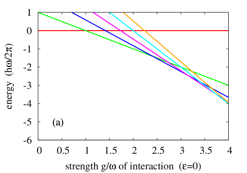
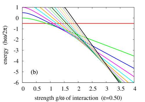
Figure 2: Energy-level crossings among $E_{\nu}^{\mathrm{g}}(\varepsilon)$, $\nu=0,\pm 1,\pm 2,\cdots$, of the parameterized JC Hamiltonian. Each color indicates individual index $\nu$ of the energy $E_{\nu}^{\mathrm{g}}(\varepsilon)$. Here $\omega_{\mathrm{a}}=\omega_{\mathrm{c}}=\omega$. (a) $E_{\nu}^{\mathrm{g}}(\varepsilon)$, $\nu=0,-1,-2,\cdots$, of the standard JC model ($\varepsilon=0$); (b) $E_{\nu}^{\mathrm{g}}(\varepsilon)$, $\nu=0,-1,-2,\cdots$, of the parameterized JC model ($\varepsilon=0.50$); (c) $E_{\nu}^{\mathrm{g}}(\varepsilon)$, $\nu=0,\pm 1,\pm 2,\cdots$, of the parameterized JC model ($\varepsilon=0.50$). Here, for each $|\nu|$, $E_{\pm|\nu|}^{\mathrm{g}}(\varepsilon)$ are drawn with the same color, but $E_{+|\nu|}^{\mathrm{g}}(\varepsilon)$ and $E_{-|\nu|}^{\mathrm{g}}(\varepsilon)$ are respectively described by the dotted line and the solid one.

These energy-level crossings supply us with the envelope by the energies, which makes the ground-state energy with the order $2$. This phenomenon is caused by many GSTs: We can prove that the eigenstate $\varphi_{0}^{\mathrm{g}}(\varepsilon)$ with the eigenenergy $E_{0}^{\mathrm{g}}(\varepsilon)$ is the ground state for the coupling strength less than a critical coupling strength, but the eigenstate $\varphi_{-1}^{\mathrm{g}}(\varepsilon)$ with the eigenenergy $E_{-1}^{\mathrm{g}}(\varepsilon)$ replaces the old ground state $\varphi_{0}^{\mathrm{g}}(\varepsilon)$ and becomes the new ground state for the coupling strength more than the critical point. At the critical point, the parameterized JC Hamiltonian has degenerate ground states. Each eigenstate $\varphi_{-|\nu|}^{\mathrm{g}}(\varepsilon)$ with the energy $E_{-|\nu|}^{\mathrm{g}}(\varepsilon)$, $|\nu|=1,2,\cdots$, also becomes the ground state in turn as the coupling strength grows larger and larger, though it is primarily an excited state. We consequently note that we can also find the ground-state entanglement property [38] in this process (see §8).

We make more mathematical statements on the GST here. We define the quantity $G_{|\nu|}(\varepsilon)$ by

$$G_{|\nu|}(\varepsilon):=(1-\varepsilon)^{2}\omega^{2}\left[|\nu|+\frac{\Delta_{\varepsilon}}{\left(1-\varepsilon\right)\omega}\right].$$ (24)

Let us now denote by the symbol $\sharp$ the equal sign $=$, the inequality sign $>$, or the inequality sign $<$. Then, in the same way as in Ref.[36], the direct computation immediately brings us the necessary and sufficient condition:

$$E_{0}^{\mathrm{g}}(\varepsilon)\,\sharp\,E_{-|\nu|}^{\mathrm{g}}(\varepsilon)\,\,\,\text{if and only if}\,\,\,\mathrm{g}^{2}\,\sharp\,G_{|\nu|}(\varepsilon).$$ (25)

In the case $\varepsilon=0$, it is easy to compare the two energies $E_{-|\nu|+1}^{\mathrm{g}}(0)$ and $E_{-|\nu|}^{\mathrm{g}}(0)$:

$$E_{-|\nu|+1}^{\mathrm{g}}(0)\,\sharp\,E_{-|\nu|}^{\mathrm{g}}(0)\quad\text{if and only if}\quad\mathrm{g}\,\sharp\,(\sqrt{|\nu|}+\sqrt{|\nu|-1})\omega$$ (26)

for $|\nu|=1,2,\cdots$.

5 GST indices and CQPT

In this section we introduce the GST indices (GSTI) to see the CQPT for the Rabi model.

We give the transition probability amplitudes $A_{\nu}$ and $B_{\nu}$ by

$$\begin{cases}A_{\nu}:=\langle\varphi_{\nu}^{\mathrm{g}}(\varepsilon)|\varphi_{\mathrm{Rabi}}\rangle,\\ B_{\nu}:=\langle\sigma_{x}\varphi_{\nu}^{\mathrm{g}/\varepsilon}(0)|\varphi_{\mathrm{Rabi}}\rangle,\end{cases}\nu=0,\pm 1,\pm 2,\cdots,$$

for the normalized ground state $\varphi_{\mathrm{Rabi}}$ of the Rabi Hamiltonian and normalized eigenstates $\varphi_{\nu}^{\mathrm{g}}(\varepsilon)$ and $\varphi_{\nu}^{\mathrm{g}/\varepsilon}(0)$ of the parameterized JC Hamiltonians. As proved in §C.5, the ground-state energy $E_{\mathrm{Rabi}}$ of the Rabi Hamiltonian can be expanded as:

$$E_{\mathrm{Rabi}}=\sum_{\ell\in\mathbb{Z}}\left[E_{2\ell}^{\mathrm{g}}(\varepsilon)|A_{2\ell}|^{2}+\varepsilon E_{2\ell+1}^{\mathrm{g}/\varepsilon}(0)|B_{2\ell+1}|^{2}\right],$$ (27)

where $\mathbb{Z}$ denotes the set of all integers. We are interested in which term is dominant in the expansion (27). If we grasped the transition probabilities $|A_{2\ell}|^{2}$ and $|B_{2\ell+1}|^{2}$, we could understand how the effect from the chiral space contributes to the ground-state energy of the Rabi Hamiltonian. But, unfortunately, we have not developed such mathematics to grasp them yet. Thus, we employ another way.

We define the lowest-energy sum $E_{\mathrm{les}}(\varepsilon)$ by the sum of two ground-state energies of chiral pair Hamiltonians of the Rabi model:

$$E_{\mathrm{les}}(\varepsilon):=E_{\mathrm{JC}}^{\mathrm{g}}(\varepsilon)+\varepsilon E_{\mathrm{JC}}^{\mathrm{g}/\varepsilon}(0).$$ (28)

Here $E_{\mathrm{JC}}^{\mathrm{g}}(\varepsilon)$ and $E_{\mathrm{JC}}^{\mathrm{g}/\varepsilon}(0)$ were respectively ground-state energies of the standard part $H_{\mathrm{JC}}^{\mathrm{g}}(\varepsilon)$ of the chiral pair Hamiltonians and its chiral-counter Hamiltonian $H_{\mathrm{JC}}^{\mathrm{g}/\varepsilon}(0)$. As already explained in §4, the GST takes place for the individual parameterized JC Hamiltonians, $H_{\mathrm{JC}}^{\mathrm{g}}(\varepsilon)$ and $H_{\mathrm{JC}}^{\mathrm{g}_{\varepsilon}}(0)$, when the coupling strength is large. Thus, we indicate them as $E_{\nu_{*}}^{\mathrm{g}}(\varepsilon):=E_{\mathrm{JC}}^{\mathrm{g}}(\varepsilon)$ and $E_{\nu_{**}}^{\mathrm{g}/\varepsilon}(0):=E_{\mathrm{JC}}^{\mathrm{g}/\varepsilon}(0)$ with proper non-positive integers $\nu_{*}$ and $\nu_{**}$, and we can rewrite the lowest-energy sum as:

$$E_{\mathrm{les}}(\varepsilon)=E_{\nu_{*}}^{\mathrm{g}}(\varepsilon)+\varepsilon E_{\nu_{**}}^{\mathrm{g}/\varepsilon}(0).$$ (29)

We call the pair $[\,|\nu_{*}|\,,\,|\nu_{**}|\,](\varepsilon)$ of non-negative integers $|\nu_{*}|$ and $|\nu_{**}|$ the GSTI for the decomposition rate $\varepsilon$. In the case where the ground-state energy of the parameterized JC Hamiltonian $H_{\mathrm{JC}}^{\mathrm{g}}(\varepsilon)$ has some degenerate ground states, we employ the non-positive integer $\nu_{*}$ so that its absolute value $|\nu_{*}|$ becomes the minimum. More precisely, the argument as in §2 of Ref.[39] guarantees that each eigenstate of the parameterized JC Hamiltonian is actually unique or finitely degenerate. So, we can write $\inf\mathrm{Spec}(H_{\mathrm{JC}}^{\mathrm{g}}(\varepsilon))=E_{\nu_{j}}^{\mathrm{g}}(\varepsilon)$ for some $j=1,2,\cdots,J$. Here the notation $\mathrm{Spec}(H)$ stands for the set of the energy spectra of a Hamiltonian $H$. Thus, we can employ the non-positive integer $\nu_{*}$ satisfying $|\nu_{*}|=\min_{j=1,2,\cdots,J}|\nu_{j}|$ then. We adopt the same definition for the index $|\nu_{**}|$.

The GSTI tell us how the GST takes place: For non-negative integers $m$ and $n$, the change in GSTI from $[m,n](\varepsilon)$ to $[m+1,n](\varepsilon)$ shows that a GST takes place for the standard part of the chiral pair Hamiltonians, and the change from $[m,n](\varepsilon)$ to $[m,n+1](\varepsilon)$ means a GST for the chiral part. Actually, in the case $\nu_{*}\neq 0$ there is the following relation among the indices $|\nu_{*}|$ and $|\nu_{**}|$, and the decomposition rate $\varepsilon$ in the GSTI:

$$|\nu_{**}|+1\leq|\nu_{*}|+\frac{1}{2\varepsilon},\qquad\nu_{*},\nu_{**}=\,-1,-2,\cdots,$$ (30)

which will be proved in §C.4.

As proved in §C.2, the mathematical statements (25) and (26) lead to the following necessary and sufficient condition: Define the interval $I_{\varepsilon}$ by

$$I_{\varepsilon}:=[0\,,\,\sqrt{G_{1}(\varepsilon)}]=[0\,,\,(1-\varepsilon)\omega\sqrt{1+\Delta_{\varepsilon}/(1-\varepsilon)\omega}\,].$$ (31)

Let the decomposition rate $\varepsilon$ be in the range between $0$ and $1/2$ (i.e, $0\leq\varepsilon\leq 1/2$), and the critical coupling constant $\mathrm{g}[\varepsilon]$ be defined by $\mathrm{g}[\varepsilon]:=\varepsilon\omega$. Then, for the coupling strength $\mathrm{g}$ running over $I_{\varepsilon}$, the critical coupling strength $\mathrm{g}[\varepsilon]$ is in the interval $I_{\varepsilon}$, and

$$\begin{cases}\text{the GSTI are $[0,0](\varepsilon)$ if and only if $\mathrm{g}\leq\mathrm{g}[\varepsilon]$, and moreover,}\\ \text{the GSTI are $[0,n](\varepsilon)$ with some negative integer $n$ ($\neq 0$)}\\ \text{if and only if $\mathrm{g}>\mathrm{g}[\varepsilon]$.}\end{cases}$$ (32)

In the case $\omega_{\mathrm{a}}\neq\omega_{\mathrm{c}}$, the critical point $\mathrm{g}[\varepsilon]$ is actually $\mathrm{g}[\varepsilon]=\varepsilon\sqrt{\omega_{\mathrm{a}}\omega_{\mathrm{c}}}$. The critical point $g[0.5]$ reminds us the critical point of the Hepp-Lieb quantum phase transition [40, 41] (see the comment (48) below).

The chiral decomposition (19) says that if the standard part $H_{\mathrm{JC}}^{\mathrm{g}}(\varepsilon)$ and its chiral part $\varepsilon\sigma_{x}H_{\mathrm{JC}}^{\mathrm{g}_{\varepsilon}}(0)\sigma_{x}$ were commutable (mathematically in the sense of Definition on p.271 of Ref.[42]), then the ground-state energy $E_{\mathrm{Rabi}}$ of the Rabi Hamiltonian $H_{\mathrm{Rabi}}$ would be equal to the lowest-energy sum $E_{\mathrm{les}}(\varepsilon)$. But, unfortunately, they are not commutable in fact. We therefore define the difference $E_{\mathrm{diff}}(\varepsilon)$ between the ground-state energy of the Rabi Hamiltonian and the lowest-energy sum by $E_{\mathrm{diff}}(\varepsilon):=E_{\mathrm{Rabi}}-E_{\mathrm{les}}(\varepsilon)$, called non-commutativity energy. That is, the non-commutativity energy represents how the chiral part affects to the standard part in the ground-state energy of the Rabi model. Conversely, if the effect from the chiral part is small, the non-commutativity energy should be small. Eq.(27) leads to the expansion of the non-commutativity energy:

$$E_{\mathrm{diff}}(\varepsilon)=\sum_{\ell\in\mathbb{Z}}\left[E_{2\ell}^{\mathrm{g}}(\varepsilon)\left(|A_{2\ell}|^{2}-\delta_{(2\ell)\nu_{*}}\right)+\varepsilon E_{2\ell+1}^{\mathrm{g}/\varepsilon}(0)\left(|B_{2\ell+1}|^{2}-\delta_{(2\ell+1)\nu_{**}}\right)\right].$$

The ground-state energy of the Rabi Hamiltonian is decomposed as:

$$E_{\mathrm{Rabi}}=E_{\mathrm{JC}}^{\mathrm{g}}(\varepsilon)+\varepsilon E_{\mathrm{JC}}^{\mathrm{g}/\varepsilon}(0)+E_{\mathrm{diff}}(\varepsilon).$$ (33)

As a reminder that we follow the phenomenology coming from some experimental facts: The conditions (RWA) implies the equitableness breaking, and thus, the counter-rotating term is turned on and grows as the coupling strength gets larger and larger as if to restore the equitableness. These experimental facts say in a mathematically naive sense that the non-commutativity between the chiral pair Hamiltonians should be so small that the standard part of the lowest-energy sum plays an important role in the weak and strong coupling regime, because the chiral-counter Hamiltonian’s effect itself is too small to show up in the experimental results. We cannot, however, ignore it in the ultra-strong coupling regime.

According to these phenomenological observations, since the approximation, $E_{\mathrm{Rabi}}\approx E_{\mathrm{JC}}=E_{\mathrm{JC}}^{\mathrm{g}}(0)$, experimentally holds for the very small coupling strength (i.e., $\mathrm{g}\ll 1$), Eq.(33) makes us expect that:

$$\mathrm{g}\ll 1\,\text{implies that}\,\,\,\varepsilon\approx 0\,\,\,\text{with}\,\,\,\varepsilon E_{\mathrm{JC}}^{\mathrm{g}/\varepsilon}(0)\approx 0\,\,\,\text{and}\,\,\,E_{\mathrm{diff}}(\varepsilon)\approx 0.$$ (34)

Moreover,

$$\begin{cases}&\text{as the coupling strength $\mathrm{g}$ becomes larger, the energy}\\ &\text{$\varepsilon E_{\mathrm{JC}}^{\mathrm{g}/\varepsilon}(0)$ must appear from the chiral part, and it must}\\ &\text{increase gradually.}\end{cases}$$ (35)

In our arguments below, the statements (34) and (35) will be justified. Then, the former statement (34) is consistent with the RWA. The latter statement (35) reveals a kind of the CQPT [23]. That is, the CQPT causes the shift of the dominant part of the decomposition Eq.(33) from the standard part of the chiral pair Hamiltonians to its chiral part, which is represented by GSTI. In the process of this shift, it becomes important to grasp the behavior of the non-commutativity energy $E_{\mathrm{diff}}(\varepsilon)$ as well:

Our attempt to find the shift is not always available for all physical models. For example, let $H_{\mathrm{ho}}$ be the $1$-dimensional Schrödinger operator for the quantum harmonic oscillator: $H_{\mathrm{ho}}:=\,-(1/2)d^{2}/dx^{2}+\mathrm{g}x^{2}$. Here we set $\hbar$ as $\hbar=1$ for simplicity. Denote the ground-state energy of the Schrödinger operator $H_{\mathrm{ho}}$ by $E_{\mathrm{ho}}$ and then it is actually $\sqrt{\mathrm{g}/2}$. We set the parameterized Hamiltonian $H_{0}(\varepsilon)$ as $H_{0}(\varepsilon):=\,-\varepsilon d^{2}/dx^{2}$. We denote its ground-state energy by $E_{0}(\varepsilon)$ and then it is actually $0$. Here we meant the infimum of energies by ‘ground-state energy’ though the Hamiltonian $H_{0}(\varepsilon)$ does not have a ground state in its state space. We have the decomposition $H_{\mathrm{ho}}=H_{0}(1/2)+F^{*}H_{0}(\mathrm{g})F$ for the Fourier transform $F$. The both Hamiltonians $H_{0}(1/2)$ and $H_{0}(\mathrm{g})$ are solvable and their energies are given as $\left[\left.0,\infty\right)\right.$. Define the lowest-energy sum $E^{\mathrm{ho}}_{\mathrm{les}}(\varepsilon)$ by $E^{\mathrm{ho}}_{\mathrm{les}}(\varepsilon):=E_{0}(1/2)+E_{0}(\mathrm{g})$. Then, we can define the non-commutativity energy $E^{\mathrm{ho}}_{\mathrm{diff}}(\varepsilon)$ by $E^{\mathrm{ho}}_{\mathrm{diff}}(\varepsilon):=E_{\mathrm{ho}}-E^{\mathrm{ho}}_{\mathrm{les}}(\varepsilon)$. For this model, the lowest-energy sum is actually zero, $E^{\mathrm{ho}}_{\mathrm{les}}(\varepsilon)=0$, and we have the non-commutativity energy as $E^{\mathrm{ho}}_{\mathrm{diff}}(\varepsilon)=\sqrt{\mathrm{g}/2}$. Accordingly, the lowest-energy sum does not make sense in the ground-state energy of the Hamiltonian $H_{\mathrm{ho}}$. The non-commutativity energy plays an important role in the ground-state energy rather than the lowest-energy sum for the Hamiltonian $H_{\mathrm{ho}}$.

Therefore, we have to investigate the behavior of the non-commutativity energy for the Rabi model.

6 Estimates of Non-Commutativity Energy

In this section we study the boundedness of the non-commutativity energy for the Rabi model.

For a start, we will give the lower bound $E_{\mathrm{lbd}}^{\mathrm{g}}(\varepsilon)$ and the upper bound $E_{\mathrm{ubd}}^{\mathrm{g}}(\varepsilon)$ of the non-commutativity energy $E_{\mathrm{diff}}(\varepsilon)$ to make the estimate:

$$\max\left\{0\,,\,E_{\mathrm{lbd}}^{\mathrm{g}}(\varepsilon)\right\}\leq E_{\mathrm{diff}}(\varepsilon)\leq E_{\mathrm{ubd}}^{\mathrm{g}}(\varepsilon),$$ (36)

namely,

$$\max\left\{E_{\mathrm{les}}(\varepsilon)\,,\,E_{\mathrm{les}}(\varepsilon)+E_{\mathrm{lbd}}^{\mathrm{g}}(\varepsilon)\right\}\leq E_{\mathrm{Rabi}}\leq E_{\mathrm{les}}(\varepsilon)+E_{\mathrm{ubd}}^{\mathrm{g}}(\varepsilon).$$ (37)

So, we determine the lower bound $E_{\mathrm{lbd}}^{\mathrm{g}}(\varepsilon)$ and the upper bound $E_{\mathrm{ubd}}^{\mathrm{g}}(\varepsilon)$ now. Define two functions $e_{\mathrm{low}}(\mathrm{g})$ and $e_{\mathrm{upp}}(\mathrm{g})$ of the variable $\mathrm{g}$ by

$$e_{\mathrm{low}}(\mathrm{g}):=\,-\,\frac{\hbar\mathrm{g}^{2}}{\omega},$$

$$e_{\mathrm{upp}}(\mathrm{g}):=\frac{\hbar\omega}{2}\left(1-e^{-2\mathrm{g}^{2}/\omega^{2}}\right)-\,\frac{\hbar\mathrm{g}^{2}}{\omega}.$$

In the case $\omega_{\mathrm{a}}\neq\omega_{\mathrm{c}}$ we set the lower bound $e_{\mathrm{low}}(\mathrm{g})$ and the upper bound $e_{\mathrm{upp}}(\mathrm{g})$ as: $e_{\mathrm{upp}}(\mathrm{g}):=(\hbar\omega_{\mathrm{c}}/2)-(\hbar\mathrm{g}^{2}/\omega_{\mathrm{c}})-(\hbar\omega_{\mathrm{a}}/2)$ and $e_{\mathrm{upp}}(\mathrm{g}):=(\hbar\omega_{\mathrm{c}}/2)-(\hbar\mathrm{g}^{2}/\omega_{\mathrm{c}})-(\hbar\omega_{\mathrm{a}}/2)e^{-2\mathrm{g}^{2}/\omega_{\mathrm{c}}^{2}}$. Applying variational principle, we obtain the estimate:

$$e_{\mathrm{low}}(\mathrm{g})\leq E_{\mathrm{Rabi}}\leq e_{\mathrm{upp}}(\mathrm{g})$$ (38)

(See Fig.3(a) and (b), and §C.3 for its proof).

Let us make here a small remark. As explained in §B, for the Rabi model we can find some expressions similar to those for the instanton gas, and then, we can express the ground-state energy $E_{\mathrm{Rabi}}$ à la instanton gas, which also gives the estimate (38).

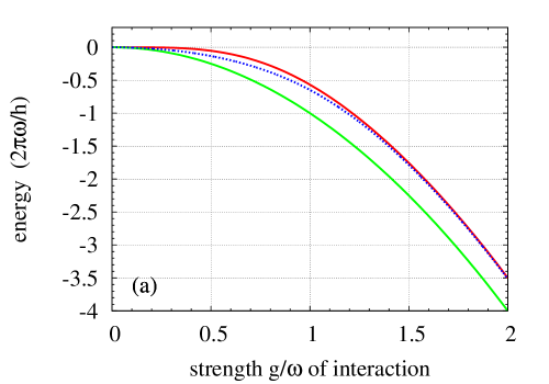
Figure 3: Set $\omega=\omega_{\mathrm{a}}=\omega_{\mathrm{c}}$. $e_{\mathrm{low}}(\mathrm{g})/\hbar\omega$(green solid line), $e_{\mathrm{upp}}(\mathrm{g})/\hbar\omega$(red solid line), numerically-calculated ground-state energy $E_{\mathrm{Rabi}}$(blue dotted line). (a) $0\leq\mathrm{g}/\omega\leq 2$; (b) $0\leq\mathrm{g}/\omega\leq 1.5$; (c) $(e_{\mathrm{upp}}(\mathrm{g})-e_{\mathrm{les}}(\mathrm{g}))/\hbar\omega$(black solid line).

The inequalities (38) bring our desired estimate for the non-commutativity energy, setting the lower bound $E_{\mathrm{lbd}}^{\mathrm{g}}(\varepsilon)$ and the upper bound $E_{\mathrm{ubd}}^{\mathrm{g}}(\varepsilon)$ as:

$$\begin{cases}E_{\mathrm{lbd}}^{\mathrm{g}}(\varepsilon):=e_{\mathrm{low}}(\mathrm{g})-E_{\mathrm{les}}(\varepsilon),\\ E_{\mathrm{ubd}}^{\mathrm{g}}(\varepsilon):=e_{\mathrm{upp}}(\mathrm{g})-E_{\mathrm{les}}(\varepsilon).\end{cases}$$ (39)

The inequalities (37) lead to the asymptotic behavior:

$$E_{\mathrm{Rabi}}\approx\frac{\hbar\omega}{2}-\hbar\frac{\mathrm{g}^{2}}{\omega}\,\,\,\text{as $\mathrm{g}\to\infty$}.$$ (40)

We can estimate the difference between the two bounds $e_{\mathrm{low}}(\mathrm{g})$ and $e_{\mathrm{upp}}(\mathrm{g})$ as:

$$0\leq e_{\mathrm{upp}}(\mathrm{g})-e_{\mathrm{low}}(\mathrm{g})\leq\frac{\hbar\omega}{2}$$

with the limit

$$\lim_{\mathrm{g}\to\infty}(e_{\mathrm{upp}}(\mathrm{g})-e_{\mathrm{low}}(\mathrm{g}))=\frac{\hbar\omega}{2}$$

(see Fig.3(c)). Namely, the difference between the two bounds, $e_{\mathrm{low}}(\mathrm{g})$ and $e_{\mathrm{upp}}(\mathrm{g})$, is less than or equal to the zero-point energy (i.e., the vacuum fluctuation).

By practically estimating the lower bound $E_{\mathrm{lbd}}^{\mathrm{g}}(\varepsilon)$ and the upper bound $E_{\mathrm{ubd}}^{\mathrm{g}}(\varepsilon)$, we can obtain the following estimates of the non-commutativity energy as in [I]–[III], which will be proved in §C.4.

[I] For the region $0\leq\mathrm{g}/\omega\leq\varepsilon<0.1$ implying the GSTI $[0,0](\varepsilon)$, we obtain the estimates:

$$0<\varepsilon\hbar\omega-\frac{\hbar\mathrm{g}^{2}}{\omega}\leq E_{\mathrm{diff}}(\varepsilon)\leq\frac{\hbar\omega}{2}(1-e^{-2\mathrm{g}^{2}/\omega^{2}})+\varepsilon\hbar\omega-\frac{\hbar\mathrm{g}^{2}}{\omega}.$$ (41)

Thus, taking the decomposition rate $\varepsilon$ as $\varepsilon=\mathrm{g}/\omega$ leads to

$$E_{\mathrm{diff}}(\mathrm{g}/\omega)\leq 0.1\hbar\omega$$ (42)

at most.

[II] For the GSTI $[0,1](\varepsilon)$ we have the estimate as:

$$\max\left\{0\,,\,\hbar\mathrm{g}-\frac{\hbar\mathrm{g}^{2}}{\omega}\right\}\leq E_{\mathrm{diff}}(\varepsilon)\leq\frac{\hbar\omega}{2}(1-e^{-2\mathrm{g}^{2}/\omega^{2}})+\hbar\mathrm{g}-\frac{\hbar\mathrm{g}^{2}}{\omega}.$$ (43)

This estimate implies at most

$$E_{\mathrm{diff}}(\varepsilon)\leq 0.53\hbar\omega.$$ (44)

[III] For for the GSTI $[\,|\nu_{*}|\,,\,|\nu_{**}|\,](\varepsilon)$ with $|\nu_{*}|\leq|\nu_{**}|+1$ for negative indices $\nu_{*},\nu_{**}=\,-1,-2,\cdots$, we can show the following estimate:

$$\max\Bigl{\{}0\,,\,\hbar\omega\Bigl{[}-|\nu_{*}|-\varepsilon(|\nu_{**}|-|\nu_{*}|)$$

$$\qquad\qquad\qquad\qquad\qquad+\sqrt{\varepsilon^{2}+\frac{\mathrm{g}^{2}}{\omega^{2}}|\nu_{*}|}+\frac{\mathrm{g}}{\omega}\sqrt{|\nu_{**}|}-\,\frac{\mathrm{g}^{2}}{\omega^{2}}\Bigr{]}\Bigr{\}}$$

$$\leq E_{\mathrm{diff}}(\varepsilon)$$

$$\leq \hbar\omega\Bigl{[}\frac{1}{2}-|\nu_{*}|-\varepsilon(|\nu_{**}|-|\nu_{*}|)$$

$$\qquad\qquad\qquad\qquad+\sqrt{\varepsilon^{2}+\frac{\mathrm{g}^{2}}{\omega^{2}}|\nu_{*}|}+\frac{\mathrm{g}}{\omega}\sqrt{|\nu_{**}|}-\,\frac{\mathrm{g}^{2}}{\omega^{2}}-\,\frac{1}{2}e^{-2\mathrm{g}^{2}/\omega^{2}}\Bigr{]}.$$ (45)

The upper bound follows from this estimate as:

$$E_{\mathrm{diff}}(\varepsilon)\leq 0.5\hbar\omega.$$ (46)

Combining the relation (30) with the condition for the statement [III], we realize the relation:

$$0<|\nu_{*}|\leq|\nu_{**}|+1\leq|\nu_{*}|+\frac{1}{2\varepsilon}.$$ (47)

The upper bound $E_{\mathrm{ubd}}^{\mathrm{g}}(\varepsilon)$ is numerically estimated as in Fig.4(a).

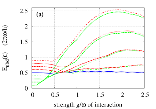
Figure 4: (a) $E_{\mathrm{ubd}}^{\mathrm{g}}(\varepsilon)/\hbar\omega$. From the bottom at $\mathrm{g}/\omega=0$, $\varepsilon=0.10$(green dashed line); $\varepsilon=0.20$(green dashed-dotted line); $\varepsilon=0.30$(green dotted line); $\varepsilon=0.40$(green dotted-dotted line); $\varepsilon=0.50$(blue solid line); $\varepsilon=0.60$(red dashed line); $\varepsilon=0.70$(red dashed-dotted line); $\varepsilon=0.80$(red dotted line); $\varepsilon=0.90$(red dotted-dotted line). The envelope of all lines gives a better value of $E_{\mathrm{ubd}}^{\mathrm{g}}(\varepsilon)/\hbar\omega$. (b) $(E_{\mathrm{les}}(0.5)+0.51\hbar\omega-E_{\mathrm{Rabi}})/\hbar\omega$ (black solid line), where $E_{\mathrm{Rabi}}$ is the numerically computed ground-state energy.

The numerical results in Fig.4 say that the non-commutativity energy $E_{\mathrm{diff}}(\varepsilon)$ is almost bounded by the fluctuation of vacuum from above for the coupling strength less than $\mathrm{g}/\omega=2.5$. In particular, the numerical analyses in Fig.4(b) say that we can make the difference between the two energies, $E_{\mathrm{Rabi}}$ and $E_{\mathrm{les}}(0.5)+E_{\mathrm{diff}}(\varepsilon)$, is almost less than $0.01\hbar\omega$ if we take the non-commutativity energy $E_{\mathrm{diff}}(\varepsilon)$ as in Fig.4(b) for the region $0.5\precsim\mathrm{g}/\omega\precsim 2.5$. Here we point out that

$$\begin{cases}&\text{the value of the decomposition rate, $\varepsilon=0.5$, means that}\\ &\text{the chiral pair Hamiltonians share the SUSY Hamiltonian}\\ &\text{$H_{\mathrm{SS}}$ with each other fairly since $\omega_{\mathrm{a}}(0.5)=\omega_{\mathrm{c}}(0.5)=0.5\omega$.}\end{cases}$$ (48)

In addition to an upper bound of the non-commutativity energy, we have a lower bound from our numerical result: Fig.3(b) gives us the inequality $E_{\mathrm{ubd}}^{\mathrm{g}}(\varepsilon)-E_{\mathrm{diff}}(\varepsilon)=e_{\mathrm{upp}}(\mathrm{g})-E_{\mathrm{Rabi}}\precsim 0.1\hbar\omega$. Since the non-commutativity energy is non-negative (e.g., see the last inequality in §C.4), we obtain the lower bound as $\max\{0,E_{\mathrm{ubd}}^{\mathrm{g}}(\varepsilon)-0.1\hbar\omega\}\precsim E_{\mathrm{diff}}(\varepsilon)$.

7 Settlement of Decomposition Rate

Introducing the decomposition rate $\varepsilon$ gives the degree of freedom of the curvature to the energy-curve of the parameterized JC Hamiltonian. For example, compare the ground-state energy curves in Fig.2. In fact, we obtain too many degrees of freedom of the curvature to determine the best decomposition rate $\varepsilon$. Judging from the condition (34) and the boundedness in [I]–[III], one of candidates of the best decomposition rate may be the minimizer $\varepsilon_{*}$:

$$E_{\mathrm{diff}}(\varepsilon_{*})=\inf_{0<\varepsilon<1}E_{\mathrm{diff}}(\varepsilon).$$

Unfortunately there has not yet been an answer to this problem on seeking the minimizer $\varepsilon_{*}$. It is thus important to find a better decomposition rate $\varepsilon$ as far as we can at the present stage in order that we study the CQPT in the next section. We here propose a temporary criterion: When fixing the coupling constant $\mathrm{g}$ arbitrarily, we chose a decomposition rate $\varepsilon$ so that the non-commutativity energy $E_{\mathrm{diff}}(\varepsilon)$ becomes as small as possible.

By our results in mathematics or numeral analysis argued in preceding sections, we can take a better concrete decomposition rate $\varepsilon$ as $\varepsilon=\mathrm{g}/\omega$ for the weak and strong coupling regimes because any decomposition rate $\varepsilon$ satisfies $0\leq\mathrm{g}/\omega\leq\varepsilon<0.1$ in these regimes. When the coupling constant $\mathrm{g}$ is arbitrarily given in the ultra-strong coupling regime, let us chose a better decomposition rate $\varepsilon$ among the candidates $\mathcal{E}=\left\{0.10,0.20,\cdots,0.90\right\}$. This is because we do not have any concrete expression of the non-commutativity energy $E_{\mathrm{diff}}(\varepsilon)$, and cannot solve the mathematical problem on the minimizer $\varepsilon_{*}$ yet. We employ the decomposition rate $\varepsilon$ by the equation

$$E_{\mathrm{ubd}}^{\mathrm{g}}(\varepsilon)=\min_{\varepsilon^{\prime}\in\mathcal{E}}E_{\mathrm{ubd}}^{\mathrm{g}}(\varepsilon^{\prime})$$ (49)

instead. We obtain the concrete decomposition rates $\varepsilon$ as in Table 1. Of course, we can find a better candidate $\varepsilon$ than ours if we enlarge the set $\mathcal{E}$.

range of coupling strength	value of decomposition rate
$\mathrm{g}/\omega$	$\varepsilon$
$0\leq\mathrm{g}/\omega\leq\varepsilon<0.1$	$\mathrm{g}/\omega$
$0.1\leq\mathrm{g}/\omega<0.2414$	$0.10$
$0.2414\leq\mathrm{g}/\omega<0.4$	$0.20$
$0.4\leq\mathrm{g}/\omega<0.5$	$0.30$
$0.5\leq\mathrm{g}/\omega<0.9165$	$0.40$
$0.9165\leq\mathrm{g}/\omega<0.9659$	$0.40$
$0.9659\leq\mathrm{g}/\omega<1.193$	$0.50$

Table 1: The decomposition rate $\varepsilon$ defined by Eq.(49).

8 CQPT in Rabi Model

In this section we investigate how the CQPT in the Rabi model takes place using the concrete decomposition rate $\varepsilon$ obtained in the preceding section.

To begin with, we compute the GSTI for each decomposition rate $\varepsilon$ corresponding the individual coupling strength. Then, we can obtain the ground-state energies of the chiral pair Hamiltonians as in Table 2.

coupling strength	GSTI	standard part energy	chiral part energy
$\mathrm{g}/\omega$	$[\,|\nu_{*}|\,,\,|\nu_{**}|\,](\varepsilon)$	$E_{\nu_{*}}^{\mathrm{g}}(\varepsilon)$	$\varepsilon E_{\nu_{**}}^{\mathrm{g}/\varepsilon}(0)$
$0\leq\mathrm{g}/\omega\leq\varepsilon<0.1$	$[0,0](\mathrm{g}/\omega)$	$-\hbar\mathrm{g}$	$0$
$0.1\leq\mathrm{g}/\omega<0.2414$	$[0,1](0.10)$	$-0.10\hbar\omega$	$0.10\hbar\omega-\hbar\mathrm{g}$
$0.2414\leq\mathrm{g}/\omega<0.4$	$[0,1](0.20)$	$-0.20\hbar\omega$	$0.20\hbar\omega-\hbar\mathrm{g}$
$0.4\leq\mathrm{g}/\omega<0.5$	$[0,1](0.30)$	$-0.30\hbar\omega$	$0.30\hbar\omega-\hbar\mathrm{g}$
$0.5\leq\mathrm{g}/\omega<0.9165$	$[0,1](0.40)$	$-0.40\hbar\omega$	$0.40\hbar\omega-\hbar\mathrm{g}$
$0.9165\leq\mathrm{g}/\omega<0.9659$	$[1,1](0.40)$	$0.6\hbar\omega-\hbar\sqrt{0.16\omega^{2}+\mathrm{g}^{2}}$	$0.40\hbar\omega-\hbar\mathrm{g}$
$0.9659\leq\mathrm{g}/\omega<1.193$	$[1,1](0.50)$	$0.5\hbar\omega-\hbar\sqrt{0.25\omega^{2}+\mathrm{g}^{2}}$	$0.50\hbar\omega-\hbar\mathrm{g}$

Table 2: GSTI and ground-state energies of Hamiltonians of chiral pair.

The results in Table 2 say that CQPT takes place when the coupling regime changes from the strong coupling regime to the ultra-strong one. In addition to this, we can find another transition at around $\mathrm{g}/\omega\approx 1.0$, namely, when the coupling strength $\mathrm{g}$ almost plunges into the deep-strong coupling regime.

8.1 Weak and Strong Coupling Regimes

In these coupling regimes, the index $|\nu_{*}|$ is zero (i.e., $\nu_{*}=0$) according to Table 2. So, the ground state of the standard part $H_{\mathrm{JC}}^{\mathrm{g}}(\varepsilon)$ is a separable state $\varphi_{0}^{\mathrm{g}}(\varepsilon)\equiv|g,0\rangle\equiv|g\rangle\otimes|0\rangle$ in the standard state space. The eigenenergy of the state $\varphi_{0}^{\mathrm{g}}(\varepsilon)$ is $E_{\mathrm{JC}}^{\mathrm{g}}(\varepsilon)=\,-\varepsilon\hbar\omega=\,-\hbar\mathrm{g}$ since $\varepsilon=\mathrm{g}/\omega$. Although the chiral part $\varepsilon\sigma_{x}H_{\mathrm{JC}}^{\mathrm{g}/\varepsilon}(0)\sigma_{x}$ also has a separable state $\sigma_{x}\varphi_{0}^{\mathrm{g}/\varepsilon}(0)$ due to $\nu_{**}=0$, the expansion (27) says that the state $\sigma_{x}\varphi_{0}^{\mathrm{g}/\varepsilon}(0)$ in the chiral state space makes no contribution in the ground-state energy of the Rabi Hamiltonian. Actually, the ground-state energy of the chiral part is zero in our case: $\varepsilon E_{\mathrm{JC}}^{\mathrm{g}/\varepsilon}(0)=0$. Thus, the growth by the coupling strength $\mathrm{g}$ in the ground-state energy $E_{\mathrm{Rabi}}$ appears from standard part only, not from the chiral part. Accordingly, the following expression works in these two regimes:

$$E_{\mathrm{Rabi}}=E_{\mathrm{JC}}^{\mathrm{g}}(\varepsilon)+E_{\mathrm{diff}}(\varepsilon)=E_{\mathrm{JC}}^{\mathrm{g}}(\mathrm{g}/\omega)+E_{\mathrm{diff}}(\mathrm{g}/\omega).$$ (50)

Since the decomposition rate $\varepsilon$ is now given by $\varepsilon=\mathrm{g}/\omega$, the estimate (41) says that the non-commutativity energy approaches to zero as the coupling strength decays:

$$\lim_{\mathrm{g}\to 0}E_{\mathrm{diff}}(\varepsilon)=\lim_{\mathrm{g}\to 0}E_{\mathrm{diff}}(\mathrm{g}/\omega)=0.$$ (51)

Eqs.(50) and (51) give a mathematical justification for the RWA so that the ground state of the Rabi Hamiltonian $H_{\mathrm{Rabi}}$ is approximated by that of the parameterized JC Hamiltonian $H_{\mathrm{JC}}^{\mathrm{g}}(\varepsilon)$, the standard part of the chiral pairs, in the weak and strong coupling regimes.

As for the ground state itself, we can make the following argument on the transition probability amplitude $A_{0}$. By using a mathematical technique [39], we can show the following estimate:

$$1-\frac{\mathrm{g}^{2}}{\omega^{2}}\leq|A_{0}|^{2}\leq 1,$$ (52)

of which proof is in §C.5. This implies the limit, $\lim_{\mathrm{g}\to 0}|A_{0}|^{2}=1$. Meanwhile, the Rabi Hamiltonian $H_{\mathrm{Rabi}}$ converges to the free Hamiltonian $(\hbar\omega/2)\sigma_{z}+\hbar\mathrm{g}(a^{\dagger}a+1/2)$ as $\mathrm{g}\to 0$ in the norm resolvent sense. Applying Lemma 4.9 of Ref.[39] or Theorem VIII.23 of Ref.[42] to this limit, we reach the ground-state limit:

$$\lim_{\mathrm{g}\to 0}\psi_{\mathrm{Rabi}}=|g,0\rangle\equiv|g\rangle|0\rangle.$$ (53)

Based on the arguments above, the dominant part of the ground state of the Rabi Hamiltonian is the separable state $|g,0\rangle\equiv|g\rangle|0\rangle$ in the weak coupling regime. Since the limit $\lim_{\mathrm{g}\to 0}E_{\mathrm{JC}}^{\mathrm{g}}(\mathrm{g}/\omega)=E_{\mathrm{JC}}$ is obtained, our method also reestablishes the well-known approximation:

$$E_{\mathrm{Rabi}}\approx E_{\mathrm{JC}},\quad 0\leq\mathrm{g}/\omega\ll 1,\qquad$$ (54)

which is consistent with the validity of the RWA under the condition (RWA).

In the case $\omega_{\mathrm{a}}\neq\omega_{\mathrm{c}}$, the expressions of $E_{\mathrm{JC}}^{\mathrm{g}}(\varepsilon)$ and $\varepsilon E_{\mathrm{JC}}^{\mathrm{g}/\varepsilon}(0)$ tell us that we have to add another condition (16) to our arguments above in addition to the condition (RWA). That is, we also need the smallness, $\varepsilon|E_{\mathrm{JC}}^{\mathrm{g}/\varepsilon}(0)|\ll|E_{\mathrm{JC}}^{\mathrm{g}}(\varepsilon)|$, estimating the chiral part to be so small as

$$\varepsilon E_{\mathrm{JC}}^{\mathrm{g}/\varepsilon}(0)=\,-\varepsilon\,\frac{\hbar(\omega_{\mathrm{a}}-\omega_{\mathrm{c}})}{2}\approx 0$$ (55)

in comparison with

$$E_{\mathrm{JC}}^{\mathrm{g}}(\varepsilon)=\,-\,\frac{\hbar\Delta_{\varepsilon}}{2}=\,-\,\frac{\hbar(\omega_{\mathrm{a}}-\omega_{\mathrm{c}})}{2}-\varepsilon\,\frac{\hbar(\omega_{\mathrm{a}}+\omega_{\mathrm{c}})}{2}.$$

Under the condition (16), we reach the approximation $E_{\mathrm{Rabi}}\approx E_{\mathrm{JC}}=\,-\hbar(\omega_{\mathrm{a}}-\omega_{\mathrm{c}})/2$ for $0\leq\mathrm{g}/\omega\ll 1$. Therefore, in our argument, the requirement of the condition (16) comes from the smallness of chiral part. In the standard interpretation for the RWA, the condition (16) is usually used for neglecting the counter-rotating term $W_{\mathrm{CR}}$ after approximating the Heisenberg pictures $e^{itH_{\mathrm{Rabi}}}We^{-itH_{\mathrm{Rabi}}}$ of the rotating and counter-rotating terms, $W=W_{\mathrm{R}},W_{\mathrm{CR}}$, for the Rabi Hamiltonian $H_{\mathrm{Rabi}}$ by the Heisenberg pictures $e^{itH_{\mathrm{SS}}}We^{-itH_{\mathrm{SS}}}$ for the free Hamiltonian $H_{\mathrm{SS}}$.

When the coupling strength grows in the weak and strong coupling regimes, the ground-state energy $E_{\mathrm{JC}}$ of the original JC Hamiltonian is beginning to produce deviation from the ground-state energy $E_{\mathrm{Rabi}}$ of the Rabi Hamiltonian. But, since the ground-state energy of the Rabi Hamiltonian still has the expression (50) as far as in the strong coupling regime, we can make corrections for the deviation by the difference between the ground-state energies of the original and parameterized JC Hamiltonians, and the non-commutativity energy. Namely, the deviation is represented as:

$$E_{\mathrm{Rabi}}-E_{\mathrm{JC}}=(E_{\mathrm{JC}}^{\mathrm{g}}(\varepsilon)-E_{\mathrm{JC}})+E_{\mathrm{diff}}(\varepsilon)$$ (56)

in the strong coupling regime as well as in the weak one. In this stage, we do not have to consider the contribution from the chiral part (i.e., the effect of the counter-rotating terms).

8.2 Ultra-Strong Coupling Regime

Table 2 says that the index $|\nu_{**}|$ of the GSTI becomes one (i.e., $\nu_{**}=\,-1$) for the region $0.1<\mathrm{g}/\omega<0.9165$. That is, the chiral-counter Hamiltonian $\varepsilon\sigma_{x}H_{\mathrm{JC}}^{\mathrm{g}/\varepsilon}(0)\sigma_{x}$ has a GST, and then, its ground state is $\varphi_{-1}^{\mathrm{g}/\varepsilon}(0)\equiv-\,\sin\theta_{0}^{\mathrm{g}/\varepsilon}(0)|e,0\rangle+\cos\theta_{0}^{\mathrm{g}/\varepsilon}(0)|g,1\rangle$ in the chiral state space, which is an entangled state and dressed with one photon. Therefore, the chiral part energy $\varepsilon E_{\mathrm{JC}}^{\mathrm{g}/\varepsilon}(0)$ is turned on and works with the expression $\varepsilon E_{\mathrm{JC}}^{\mathrm{g}/\varepsilon}(0)=\varepsilon\hbar\omega-\hbar\mathrm{g}$. This shows how the effect of the chiral part appears. On the other hand, the ground-state energy $E_{\mathrm{JC}}^{\mathrm{g}}(\varepsilon)$ is given by $E_{\mathrm{JC}}^{\mathrm{g}}(\varepsilon)=\,-\varepsilon\hbar\omega$ as before since the index $|\nu_{*}|$ is still zero. Thus, the ground-state energy $E_{\mathrm{Rabi}}$ of the Rabi Hamiltonian has the expression:

$$E_{\mathrm{Rabi}}=E_{\mathrm{JC}}^{\mathrm{g}}(\varepsilon)+\varepsilon E_{\mathrm{JC}}^{\mathrm{g}/\varepsilon}(0)+E_{\mathrm{diff}}(\varepsilon)=\,-\hbar\mathrm{g}+E_{\mathrm{diff}}(\varepsilon)$$ (57)

with

$$\begin{cases}E_{\mathrm{JC}}^{\mathrm{g}}(\varepsilon)=\,-\varepsilon\hbar\omega,\\ \varepsilon E_{\mathrm{JC}}^{\mathrm{g}/\varepsilon}(0)=\varepsilon\hbar\omega-\hbar\mathrm{g}=\,-E_{\mathrm{JC}}^{\mathrm{g}}(\varepsilon)-\hbar\mathrm{g},\\ 0\leq E_{\mathrm{diff}}(\varepsilon)\leq\text{the upper bound in the estimate (\ref{eq:lu-estimate-u1}) },\end{cases}$$

for $0.1\leq\mathrm{g}/\omega\precsim 0.9$ (See Fig.4). The energy $\varepsilon E_{\mathrm{JC}}^{\mathrm{g}/\varepsilon}(0)$ from the chiral part and the non-commutativity energy $E_{\mathrm{diff}}(\varepsilon)$ between the standard part and the chiral part arise and play an essential role. The energy $\varepsilon E_{\mathrm{JC}}^{\mathrm{g}/\varepsilon}(0)$ from the chiral part kills the energy $E_{\mathrm{JC}}^{\mathrm{g}}(\varepsilon)$ from the standard part, and it, together with the non-commutativity energy $E_{\mathrm{diff}}(\varepsilon)$, makes the effect of the coupling strength $\mathrm{g}$ in the ground-state energy $E_{\mathrm{Rabi}}$ as follows: $\max\{-\hbar\mathrm{g},-\hbar\mathrm{g}^{2}/\omega\}\leq E_{\mathrm{Rabi}}\leq\hbar(1-e^{-2\mathrm{g}^{2}/\omega^{2}})/2-\hbar\mathrm{g}^{2}/\omega$. Here, the energy $E_{\mathrm{JC}}^{\mathrm{g}}(\varepsilon)$ from the standard part makes no contribution in the ground-state energy of the Rabi model. Therefore, we can say that the effect from the chiral part begins to appear and takes the initiative in the ground-state energy of the Rabi Hamiltonian in the region of $0.1\precsim\mathrm{g}/\omega\precsim 0.9$.

9 Conclusion

We conclude this paper by summarizing how the CQPT is caused in the Rabi model by the GSTs occurring in the standard part and the chiral part of the chiral pair Hamiltonians.

We have showed that the growth of the coupling strength in the Rabi model plays a role of taking the $N=2$  SUSY to the spontaneous SUSY breaking. This spontaneous symmetry breaking is caused by the spin-chirality. In the process of the growth of the coupling strength, the spin-chirality makes the CQPT: While the contribution from the chiral part is so small that we can ignore it in the weak coupling regime as in Eq.(54), the deviation appears like Eq.(56) when the coupling strength grows in the strong coupling regime. The contribution from the chiral part is turned on and grows as in Eq.(57) in the ultra-strong coupling regime. When the coupling strength plunges into the ultra-strong coupling regime from the strong coupling regime, the GST takes place in the chiral part of the Rabi Hamiltonian. In association with this GST, as explained in §8, the ground state of the chiral-counter Hamiltonian changes from the separate state $\varphi_{0}^{\mathrm{g}/\varepsilon}(0)$ to the entangled state $\varphi_{-1}^{\mathrm{g}/\varepsilon}(0)$. The growth in the coupling strength of the ground state energy of the Rabi Hamiltonian is completely governed by the contribution from the chiral part until $\mathrm{g}/\omega\approx 0.9$. This is the explanation of the transition from the strong coupling regime to the ultra-strong one by the CQPT. We note that we can also find the almost same CQPT properties even in the case $\omega_{\mathrm{a}}\neq\omega_{\mathrm{c}}$ with the condition (16).

Acknowledgment

The author acknowledges the support from JSPS, Grant-in-Aid for Scientific Research (C) 23540204. He expresses special thanks to Pierre-Marie Billangeon and Yasunobu Nakamura for useful discussions, which aroused the author’s interest in the problems in this paper. He is also grateful to Hans Mooij, Kae Nemoto, Kouichi Semba, Enrique Solano, and Tsuyoshi Yamamoto for useful discussions on theoretical and experimental aspects of circuit QED.

Appendix A A Mathematical Justification of Asymptotic Behavior of Rabi Hamiltonian

In this appendix, we mathematically justify the asymptotic behavior (8).

For every $z\in\mathbb{C}\setminus\mathbb{R}$, we can obtain the difference between the resolvent $\left(U_{\mathrm{g}}^{*}\left(H_{\mathrm{Rabi}}+\hbar\mathrm{g}^{2}/\omega\right)U_{\mathrm{g}}-z\right)^{-1}$ and the resolvent $(\widetilde{H}_{0}-z)^{-1}$ by using the second resolvent equation along with Eq.(4):

$$\frac{1}{\widetilde{H}_{0}-z}\,-\,\frac{1}{U_{\mathrm{g}}^{*}\left(H_{\mathrm{Rabi}}+\hbar\mathrm{g}^{2}/\omega\right)U_{\mathrm{g}}-z}$$

$$= \,-\,\frac{1}{\widetilde{H}_{0}-z}\left(\frac{\hbar\omega}{2}\widetilde{V}_{\mathrm{g}}\right)\frac{1}{U_{\mathrm{g}}^{*}\left(H_{\mathrm{Rabi}}+\hbar\mathrm{g}^{2}/\omega\right)U_{\mathrm{g}}-z}.$$

Using this equation, Eq.(5), and the fact that the resolvent $(\widetilde{H}_{0}-z)^{-1}$ is a compact operator, Theorem VI.II of Ref.[42] yields the strong resolvent convergence:

$$\lim_{\mathrm{g}\to\infty}\frac{1}{U_{\mathrm{g}}^{*}\left(H_{\mathrm{Rabi}}+\hbar\mathrm{g}^{2}/\omega\right)U_{\mathrm{g}}-z}\psi=\frac{1}{\widetilde{H}_{0}-z}\psi$$ (58)

for every wave function $\psi$.

For any Borel set $\Omega$ of the $1$-dimensional Euclidean space $\mathbb{R}$, we denote by $P_{\mathrm{Rabi}}(\Omega)$ and $P_{0}(\Omega)$ the projection-valued measures so that

$$U_{\mathrm{g}}^{*}\left(H_{\mathrm{Rabi}}+\hbar\mathrm{g}^{2}/\omega\right)U_{\mathrm{g}}=\int_{-\infty}^{\infty}\lambda P_{\mathrm{Rabi}}(d\lambda)\quad\text{and}\quad\widetilde{H}_{0}=\int_{-\infty}^{\infty}\lambda P_{0}(d\lambda).$$

We recall the following properties. Let us denote $P_{\mathrm{Rabi}}(d\lambda)$ or $P_{0}(d\lambda)$ by $P_{\sharp}(d\lambda)$. Since both Hamiltonians $U_{\mathrm{g}}^{*}\left(H_{\mathrm{Rabi}}+\hbar\mathrm{g}^{2}/\omega\right)U_{\mathrm{g}}$ and $\widetilde{H}_{0}$ have only isolated discrete eigenvalues, if the finite interval $(\alpha,\beta)$ contains no eigenvalue, then $P_{\sharp}((\alpha,\beta))=0$. Conversely, if the interval $(\alpha,\beta)$ contains some eigenvalues, then the number of the eigenvalues is finite, and then, $P_{\sharp}((\alpha,\beta))=P_{\sharp}(\{E_{1},\cdots,E_{\ell}\})$, where $E_{1},\cdots,E_{\ell}$ are the finite eigenvalues.

Let $\left\{\alpha_{m}\right\}_{m=1}^{\infty}$ be a sequence satisfying

$$\hbar\omega\left(m-\,\frac{1}{2}\right)<\alpha_{m}<\hbar\omega\left(m+\frac{1}{2}\right).$$

Because of the estimate (38), the set $[0,\alpha_{1}]\cup\bigcup_{m=1}^{\infty}\left.\left(\alpha_{m},\alpha_{m+1}\right.\right]$ covers the set of all the energy levels of the renormalized Rabi Hamiltonian:

$$\mathrm{Spec}\,(H_{\mathrm{Rabi}}+\hbar\mathrm{g}^{2}/\omega)\subset[0,\alpha_{1}]\cup\bigcup_{m=1}^{\infty}\left.\left(\alpha_{m},\alpha_{m+1}\right.\right].$$ (59)

Here $\mathrm{Spec}\,(H)$ is the set of all energy of a Hamiltonian $H$.

For each natural number $m$, we take a positive number $\varepsilon_{m}$ so that

$$\hbar\omega\left(m-\,\frac{1}{2}\right)<\alpha_{m}-\varepsilon_{m}\quad\text{and}\quad\alpha_{m+1}+\varepsilon_{m}<\hbar\omega\left(m+1+\frac{1}{2}\right).$$

Applying Theorem VIII.24(b) of Ref.[42] to Eq.(58), we have the limit

$$\lim_{\mathrm{g}\to\infty}P_{\mathrm{Rabi}}((\alpha_{m}-\varepsilon_{m},\alpha_{m+1}+\varepsilon_{m}))\psi =P_{0}((\alpha_{m}-\varepsilon_{m},\alpha_{m+1}+\varepsilon_{m}))\psi$$

$$=P_{0}\left(\left\{\hbar\omega\left(m+\frac{1}{2}\right)\right\}\right)\psi,$$ (60)

which means that the state $P_{\mathrm{Rabi}}((\alpha_{m},\alpha_{m+1}))\psi$ converges to an eigenstate of the asymptotically free Hamiltonian $\widetilde{H}_{0}$. Meanwhile, by the contraposition of Theorem VIII.24(a) of Ref.[42], we have

$$(\alpha_{m}-\varepsilon_{m},\alpha_{m+1}+\varepsilon_{m})\cap\mathrm{Spec}\,\left(U_{\mathrm{g}}^{*}\left(H_{\mathrm{Rabi}}+\hbar\mathrm{g}^{2}/\omega\right)U_{\mathrm{g}}\right)\neq\emptyset$$ (61)

for sufficiently large $\mathrm{g}$ because we have $(\alpha_{m}-\varepsilon_{m},\alpha_{m+1}+\varepsilon_{m})\cap\mathrm{Spec}\,(\widetilde{H}_{0})=\left\{\hbar\omega\left(m+\frac{1}{2}\right)\right\}$.

For each eigenstate $\psi^{\mathrm{Rabi}}$ of the Hamiltonian $U_{\mathrm{g}}^{*}(H_{\mathrm{Rabi}}+\hbar\mathrm{g}^{2}/\omega)U_{\mathrm{g}}$, there is a natural number $n$ so that its eigenenergy is in the interval $(\alpha_{n}-\varepsilon_{n},\alpha_{n+1}+\varepsilon_{n})$, which is ensured by Eq.(59). So, we denote the eigenstate $\psi^{\mathrm{Rabi}}$ by $\psi^{\mathrm{Rabi}}_{n}$, i.e., $\psi^{\mathrm{Rabi}}_{n}:=\psi^{\mathrm{Rabi}}$. Thus, Eqs.(60) and (61) say that

$$\lim_{\mathrm{g}\to\infty}\psi^{\mathrm{Rabi}} =\lim_{\mathrm{g}\to\infty}\psi^{\mathrm{Rabi}}_{n}$$

$$=\lim_{\mathrm{g}\to\infty}P_{\mathrm{Rabi}}((\alpha_{n}-\varepsilon_{n},\alpha_{n+1}+\varepsilon_{n}))\psi^{\mathrm{Rabi}}_{n}$$

$$=P_{0}\left(\left\{\hbar\omega\left(n+\frac{1}{2}\right)\right\}\right)\psi^{\mathrm{Rabi}}_{n}\neq 0.$$ (62)

Here $P_{0}\left(\left\{\hbar\omega\left(n+\frac{1}{2}\right)\right\}\right)\psi^{\mathrm{Rabi}}_{n}$ is an eigenstate of the asymptotically free Hamiltonian $\widetilde{H}_{0}$. Consequently, we can say that for each eigenstate $\psi^{\mathrm{Rabi}}$ of the Hamiltonian $U_{\mathrm{g}}^{*}(H_{\mathrm{Rabi}}+\hbar\mathrm{g}^{2}/\omega)U_{\mathrm{g}}$, there is an eigenstate $\psi_{n}$ of the asymptotically free Hamiltonian $\widetilde{H}_{0}$ so that

$$\lim_{\mathrm{g}\to\infty}\psi^{\mathrm{Rabi}}=\psi_{n}.$$ (63)

Conversely, we can prove that for each eigenstate $\psi_{n}$ of the asymptotically free Hamiltonian $\widetilde{H}_{0}$, there is an eigenstate $\psi^{\mathrm{Rabi}}$ of the Hamiltonian $U_{\mathrm{g}}^{*}(H_{\mathrm{Rabi}}+\hbar\mathrm{g}^{2}/\omega)U_{\mathrm{g}}$ so that Eq.(63) holds in the following: Eqs.(59) and (61) ensure that for each $n$ there is an eigenstate $\psi^{\mathrm{Rabi}}$ of the Hamiltonian $U_{\mathrm{g}}^{*}(H_{\mathrm{Rabi}}+\hbar\mathrm{g}^{2}/\omega)U_{\mathrm{g}}$ so that its energy belongs to the interval $(\alpha_{n}-\varepsilon_{n},\alpha_{n+1}+\varepsilon_{n})$ for sufficiently large coupling strength. Thus, we obtain Eq.(62) again, which implies Eq.(63).

Therefore, we obtain the correspondence (8). Note Eq.(10) now. Then, we realize that we can chose $\psi_{n}$ as either of one of eigenvectors, $|n,\uparrow\rangle$ and $|n,\downarrow\rangle$, of the asymptotically free Hamiltonian $\widetilde{H}_{0}$. In addition, we can chose any eigenstate of the Hamiltonian $U_{\mathrm{g}}^{*}(H_{\mathrm{Rabi}}+\hbar\mathrm{g}^{2}/\omega)U_{\mathrm{g}}$ which converges to that $\psi_{n}$. Moreover, applying Theorem VIII.24(a) of Ref.[42], we can derive the relation,

$$\lim_{\mathrm{g}\to\infty}\left(E^{\mathrm{Rabi}}+\frac{\hbar\mathrm{g}^{2}}{\omega}\right)=\hbar\omega\left(n+\frac{1}{2}\right),$$

between all the energies $E^{\mathrm{Rabi}}$ and all the energies $\hbar\omega\left(n+\frac{1}{2}\right)$ from Eqs.(59) and (61), which implies the relation (9).

Appendix B Remarks on Relation with Instanton Gas

Since the Rabi model is the one-mode photon version of the spin-boson model, we can apply several results on the spin-boson Hamiltonian to the Rabi Hamiltonian. In Ref.[43] we gave a strict expression of the ground-state energy of the spin-boson model using the parity conservation between the Rabi Hamiltonian $H_{\mathrm{Rabi}}$ and the parity operator $\sigma_{z}(-1)^{a^{\dagger}a}$:

$$[H_{\mathrm{Rabi}},\sigma_{z}(-1)^{a^{\dagger}a}]=0.$$ (64)

The method for the expression in Ref.[43] reminds us of the computation for seeking the transition amplitude of the so-called instanton gas by the Euclidean path integral [44]. In this appendix we handle general frequencies, $\omega_{\mathrm{a}}$ and $\omega_{\mathrm{c}}$, that is, we accept the condition, $\omega_{\mathrm{a}}\neq\omega_{\mathrm{c}}$.

We define functions $I_{\mathrm{even}}(\beta)$ and $I_{\mathrm{odd}}(\beta)$ of a variable $\beta\geq 0$ by

$$I_{\mathrm{even}}(\beta):= 1+\sum_{\ell=1}^{\infty}\left(\frac{\omega_{\mathrm{a}}}{2}\right)^{2\ell}\int_{0}^{\beta}\!\!\!\!\!\!{d\beta_{1}}\int_{0}^{\beta_{1}}\!\!\!\!\!\!{d\beta_{2}}\cdots\int_{0}^{\beta_{2\ell-1}}\!\!\!\!\!\!{d\beta_{2\ell}}$$

$$\times e^{-2(\mathrm{g}^{2}/\omega_{\mathrm{c}}^{2})(2G_{\beta_{1},\cdots,\beta_{2\ell}}+2\ell)},$$

$$I_{\mathrm{odd}}(\beta):= \beta\frac{\omega_{\mathrm{a}}}{2}e^{-2(\mathrm{g}^{2}/\omega_{\mathrm{c}}^{2})}$$

$$+\sum_{\ell=1}^{\infty}\left(\frac{\omega_{\mathrm{a}}}{2}\right)^{2\ell+1}\int_{0}^{\beta}\!\!\!\!\!\!{d\beta_{1}}\int_{0}^{\beta_{1}}\!\!\!\!\!\!{d\beta_{2}}\cdots\int_{0}^{\beta_{2\ell}}\!\!\!\!\!\!{d\beta_{2\ell+1}}$$

$$\times e^{-2(\mathrm{g}^{2}/\omega_{\mathrm{c}}^{2})(2G_{\beta_{1},\cdots,\beta_{2\ell}}+2F_{\beta_{1},\cdots,\beta_{2\ell+1}}+\left(2\ell+1\right))}$$

for the sequences $\left\{G_{\beta_{1},\cdots,\beta_{2\ell}}\right\}_{\ell=1}^{\infty}$ and $\left\{F_{\beta_{1},\cdots,\beta_{2\ell+1}}\right\}_{\ell=0}^{\infty}$ given by

$$G_{\beta_{1},\cdots,\beta_{2\ell}}= \,-\,\sum_{p=1}^{\ell}e^{-(\beta_{2p-1}-\beta_{2p})\omega_{\mathrm{c}}}$$

$$+\sum_{p,q=1;p<q}^{\ell}\left(e^{-\beta_{2p-1}\omega_{\mathrm{c}}}-e^{-\beta_{2p}\omega_{\mathrm{c}}}\right)$$

$$\qquad\qquad\quad\times\left(e^{\beta_{2q-1}\omega_{\mathrm{c}}}-e^{\beta_{2q}\omega_{\mathrm{c}}}\right)\leq 0,$$

and

$$F_{\beta_{1},\cdots,\beta_{2\ell+1}}= e^{\beta_{2\ell+1}\omega_{\mathrm{c}}}\sum_{p=1}^{\ell}\left(e^{-\beta_{2p-1}\omega_{\mathrm{c}}}-e^{-\beta_{2p}\omega_{\mathrm{c}}}\right)\leq 0.$$

Then, Theorem 1.3 of Ref.[43] says that the ground-state energy of the Rabi Hamiltonian is expressed as

$$E_{\mathrm{Rabi}}=\frac{\hbar\omega_{\mathrm{c}}}{2}-\,\frac{\hbar\mathrm{g}^{2}}{\omega_{\mathrm{c}}}-\,\lim_{\beta\to\infty}\frac{\hbar}{\beta}\ln\left\{I_{\mathrm{even}}(\beta)+I_{\mathrm{odd}}(\beta)\right\}$$ (65)

for arbitrary coupling constant $\mathrm{g}$ provided that $1/2\leq\omega_{\mathrm{c}}/\omega_{\mathrm{a}}$.

Eq.(65) is strict, but the expression is very complicated because those of the functions $I_{\mathrm{even}}(\beta)$ and $I_{\mathrm{odd}}(\beta)$ are so. Thus, we can make it simpler with a constant. We modify the functions $I_{\mathrm{even}}(\beta)$ and $I_{\mathrm{odd}}(\beta)$ by replacing the constants $G_{\beta_{1},\cdots,\beta_{2\ell}}$ and $F_{\beta_{1},\cdots,\beta_{2\ell+1}}$ in them with simple constants $\ell G$ and $G/2$, respectively, for an arbitrary parameter $G$ in the closed interval $[-1,0]$:

$$I_{\mathrm{even}}^{G}(\beta):=\mathrm{cosh}\left[(\beta\omega_{\mathrm{a}}/2)e^{-2\mathrm{g}^{2}(G+1)/\omega_{\mathrm{c}}^{2}}\right],$$

$$I_{\mathrm{odd}}^{G}(\beta):=\mathrm{sinh}\left[(\beta\omega_{\mathrm{a}}/2)e^{-2\mathrm{g}^{2}(G+1)/\omega_{\mathrm{c}}^{2}}\right].$$

Then, Theorem 1.5 of Ref.[43] says that for every coupling constant $\mathrm{g}$ we can uniquely determine a constant $G(\mathrm{g})$ in the closed interval $[-1,0]$ so that the ground-state energy $E_{\mathrm{Rabi}}$ turns out to be a simple expression:

$$E_{\mathrm{Rabi}} =\frac{\hbar\omega_{\mathrm{c}}}{2}-\,\frac{\hbar\mathrm{g}^{2}}{\omega_{\mathrm{c}}}-\lim_{\beta\to\infty}\frac{\hbar}{\beta}\ln\left\{I_{\mathrm{even}}^{G(\mathrm{g})}(\beta)+I_{\mathrm{odd}}^{G(\mathrm{g})}(\beta)\right\}$$

$$=\frac{\hbar\omega_{\mathrm{c}}}{2}-\,\frac{\hbar\mathrm{g}^{2}}{\omega_{\mathrm{c}}}-\,\frac{\hbar\omega_{\mathrm{a}}}{2}\mathrm{exp}\left[-2\frac{\mathrm{g}^{2}}{\omega_{\mathrm{c}}^{2}}\left(G(\mathrm{g})+1\right)\right].$$ (66)

The constant $G(\mathrm{g})$ is determined as a solution of the equation:

$$\lim_{\beta\to\infty}\left\{\frac{I_{\mathrm{even}}(\beta)-I_{\mathrm{odd}}(\beta))}{I_{\mathrm{even}}^{G(\mathrm{g})}(\beta)-I_{\mathrm{odd}}^{G(\mathrm{g})}(\beta)}\right\}^{1/\beta}=1.$$

In fact, we have the limit $G(\mathrm{g})\to 0$ as $\mathrm{g}\to\infty$. The factor $2\hbar\mathrm{g}^{2}(G(\mathrm{g})+1)/\omega_{\mathrm{c}}^{2}$ in Eq.(66) plays a role similar to the classical action associated with a single-instanton solution (see Eq.(3.36) of Ref.[44]) in the expression of the transition amplitude. The functions $I_{\mathrm{even}}^{G(\mathrm{g})}(\beta)$ and $I_{\mathrm{odd}}^{G(\mathrm{g})}(\beta)$ correspond to Eqs.(3.41) of Ref.[44]. By taking $-1$ and $0$ as the constant $G(\mathrm{g})$ in Eq.(66), we obtain estimates (38) as the roughest estimates derived from Eq.(66).

Appendix C Proofs of Some Mathematical Statements

C.1 Proof of (23)

In this subsection we prove the estimates (23). Define the parameterized asymptotic Hamiltonian $H_{\mathrm{asym}}(\varepsilon)$ in the sense described in §2 by

$$H_{\mathrm{asym}}(\varepsilon):=\hbar\omega_{\mathrm{c}}(\varepsilon)\left(a^{\dagger}a+\frac{1}{2}\right)+\hbar\mathrm{g}\sigma_{x}\left(a^{\dagger}+a\right).$$

Then, this is decomposed as:

$$H_{\mathrm{asym}}(\varepsilon)=\frac{1}{2}\left(H_{\mathrm{JC}}^{\mathrm{g}}(\varepsilon)+\sigma_{x}H_{\mathrm{JC}}^{\mathrm{g}}(\varepsilon)\sigma_{x}\right).$$ (67)

It is easy to get the inequality:

$$E_{\mathrm{JC}}^{\mathrm{g}}(\varepsilon)\|\psi\|^{2} \leq \frac{1}{2}\left\{\langle\psi|H_{\mathrm{JC}}^{\mathrm{g}}(\varepsilon)|\psi\rangle+\langle\psi|\sigma_{x}H_{\mathrm{JC}}^{\mathrm{g}}(\varepsilon)\sigma_{x}|\psi\rangle\right\}$$

$$= \langle\psi|H_{\mathrm{asym}}(\varepsilon)|\psi\rangle,$$

where $\|\quad\|$ is the norm induced by the inner product: $\|\phi\|:=\langle\phi|\phi\rangle^{1/2}$. This inequality tells us that the ground-state energy of $H_{\mathrm{JC}}^{\mathrm{g}}(\varepsilon)$ does not exceed that of the parameterized asymptotic Hamiltonian $H_{\mathrm{asym}}(\varepsilon)$:

$$E_{\mathrm{JC}}^{\mathrm{g}}(\varepsilon)\leq\inf\mathrm{Spec}(H_{\mathrm{asym}}(\varepsilon)).$$

Using the unitary operator $U_{0}$ defined by

$$U_{0}:=\frac{1}{\sqrt{2}}(I-i\sigma_{y})=\frac{1}{\sqrt{2}}\begin{pmatrix}1&-1\\ 1&1\end{pmatrix},$$ (68)

we have

$$U_{0}^{*}H_{\mathrm{asym}}(\varepsilon)U_{0}= \frac{I+\sigma_{z}}{2}\otimes\left\{\hbar\omega_{\mathrm{a}}(\varepsilon)\left(a^{\dagger}a+\frac{1}{2}\right)+\hbar\mathrm{g}\left(a^{\dagger}+a\right)\right\}$$

$$+\frac{I-\sigma_{z}}{2}\otimes\left\{\hbar\omega_{\mathrm{a}}(\varepsilon)\left(a^{\dagger}a+\frac{1}{2}\right)-\hbar\mathrm{g}\left(a^{\dagger}+a\right)\right\}.$$ (69)

Using Eqs. (3) and (69), the ground-state energy of $H_{\mathrm{asym}}(\varepsilon)$ is expressed as:

$$\inf\mathrm{Spec}(H_{\mathrm{asym}}(\varepsilon))=\,-\,\frac{\hbar\mathrm{g}^{2}}{\omega_{\mathrm{c}}(\varepsilon)}.$$

Thus, we have our desired upper bound of $E_{\mathrm{JC}}^{\mathrm{g}}(\varepsilon)$.

We note the equation:

$$\|a\psi\|=\langle a\psi|a\psi\rangle^{1/2}=\langle\psi|a^{\dagger}a|\psi\rangle^{1/2}$$ (70)

for every state $\psi$. Noting the canonical commutation relation (CCR), $[a,a^{\dagger}]:=aa^{\dagger}-a^{\dagger}a=1$, we have the following inequality in the same way as above:

$$\|a^{\dagger}\psi\| =\langle\psi|aa^{\dagger}|\psi\rangle^{1/2}$$

$$=\left\{\|\psi\|^{2}+\langle\psi|a^{\dagger}a|\psi\rangle\right\}^{1/2}\leq\|\psi\|+\langle\psi|a^{\dagger}a|\psi\rangle^{1/2}.$$ (71)

Using the Schwarz inequality, the estimate by the operator norm $\|\quad\|_{\mathrm{op}}$, Eq.(70), and the inequality (71), we have

$$|\langle\psi|W_{\mathrm{R}}|\psi\rangle|\leq \|\psi\|\bigl{\{}\|\sigma_{-}\|_{\mathrm{op}}\|a^{\dagger}\psi\|_{\mathcal{H}}+\|\sigma_{+}\|_{\mathrm{op}}\|a\psi\|_{\mathcal{H}}\bigr{\}}$$

$$\leq \|\psi\|_{\mathcal{H}}^{2}+2\|\psi\|_{\mathcal{H}}\langle\psi|a^{\dagger}a|\psi\rangle^{1/2},$$

which implies

$$|\langle\psi|\hbar\mathrm{g}W_{\mathrm{R}}|\psi\rangle| \leq\hbar\mathrm{g}\left\{\delta\langle\psi|a^{\dagger}a|\psi\rangle+\left(1+\frac{1}{\delta}\right)\|\psi\|^{2}\right\}$$

$$\leq\frac{\delta\mathrm{g}}{\omega_{\mathrm{c}}(\varepsilon)}\langle\psi|H_{0}(\varepsilon)|\psi\rangle+\hbar\mathrm{g}\left\{\frac{\delta\omega_{\mathrm{a}}(\varepsilon)}{2\omega_{\mathrm{c}}(\varepsilon)}+\left(1+\frac{1}{\delta}\right)\right\}\|\psi\|^{2}$$ (72)

for every $\delta>0$. Here the parameterized free Hamiltonian $H_{0}(\varepsilon)$ was defined in Eq.(18), and we used the fact that $(\hbar\omega_{\mathrm{a}}(\varepsilon)/2)\sigma_{z}\geq-\hbar\omega_{\mathrm{a}}(\varepsilon)/2$. The inequality (72) leads to

$$\langle\psi|H_{\mathrm{JC}}^{\mathrm{g}}(\varepsilon)|\psi\rangle= \langle\psi|H_{0}(\varepsilon)|\psi\rangle+\langle\psi|\hbar\mathrm{g}W_{\mathrm{R}}\psi\rangle$$

$$\geq \langle\psi|H_{0}(\varepsilon)|\psi\rangle-|\langle\psi|\hbar\mathrm{g}W_{\mathrm{R}}|\psi\rangle|$$

$$\geq \left(1-\frac{\delta\mathrm{g}}{\omega_{\mathrm{c}}(\varepsilon)}\right)\langle\psi|H_{0}(\varepsilon)|\psi\rangle$$

$$\qquad-\hbar\mathrm{g}\left\{\frac{\delta\omega_{\mathrm{a}}\left(\varepsilon\right)}{2\omega_{\mathrm{c}}\left(\varepsilon\right)}+\left(1+\frac{1}{\delta}\right)\right\}\|\psi\|^{2}$$

Take $\delta$ as $\delta=\omega_{\mathrm{c}}(\varepsilon)/\mathrm{g}$ now. Then, we eventually reach the inequality:

$$-\,\frac{\hbar\omega_{\mathrm{a}}(\varepsilon)}{2}-\hbar\mathrm{g}-\,\frac{\hbar\mathrm{g}^{2}}{\omega_{\mathrm{c}}(\varepsilon)}\leq\frac{\langle\psi|H_{\mathrm{JC}}^{\mathrm{g}}(\varepsilon)|\psi\rangle}{\|\psi\|_{\mathcal{H}}^{2}},$$

which implies our desired lower bound of $E_{\mathrm{JC}}^{\mathrm{g}}(\varepsilon)$.

C.2 Proof of (32)

We assume that the coupling strength $\mathrm{g}$ runs over the interval $I_{\varepsilon}$ defined in Eq.(31) to prove the statement (32). So, the coupling strength $\mathrm{g}$ satisfies $\mathrm{g}^{2}\leq G_{1}(\varepsilon)$. Here the quantity $G_{|\nu|}(\varepsilon)$ was defined in Eq.(24). Since we immediately have the equation, $G_{|\nu|+1}(\varepsilon)-G_{|\nu|}(\varepsilon)=(1-\varepsilon)^{2}\omega^{2}>0$, we reach the inequality,

$$G_{|\nu|}(\varepsilon)<G_{|\nu|+1}(\varepsilon),\qquad\nu=\,-1,-2,\cdots.$$ (73)

Thus, since the condition $\mathrm{g}^{2}<\varepsilon^{2}G_{|\nu|}(\varepsilon)$ always holds for every coupling strength $\mathrm{g}\in I_{\varepsilon}$ and each $\nu=-2,-3,\cdots$ by the inequality (73), we realize that

$$\nu_{*}=0\quad\textrm{as long as $\mathrm{g}\in I_{\varepsilon}$}.$$ (74)

In addition, the mathematical fact (25) and the inequality (73) say that $E_{0}^{\mathrm{g}}(\varepsilon)<E_{-|\nu|}^{\mathrm{g}}(\varepsilon)$ for all $\nu=\,-1,-2,\cdots$.

We pay our attention to the case $\varepsilon=0$ now. Then, the mathematical fact (25) also says that there is a strictly negative integer $\nu$ so that $E_{0}^{\mathrm{g}}(0)>E_{-|\nu|}^{\mathrm{g}}(0)$ if and only if $\mathrm{g}^{2}>G_{1}(0)$. Thus, applying this fact to the chiral-counter Hamiltonian $H_{\mathrm{JC}}^{\mathrm{g}/\varepsilon}(0)$, the index $\nu_{**}$ of the GSTI satisfies

$$\begin{cases}\nu_{**}=0\quad\textrm{if and only if $\mathrm{g}^{2}/\varepsilon^{2}\leq G_{1}(0)=\omega^{2}$},\\ \nu_{**}<0\quad\textrm{if and only if $\mathrm{g}^{2}/\varepsilon^{2}>G_{1}(0)=\omega^{2}$}.\end{cases}$$ (75)

Meanwhile, we have

$$G_{1}(\varepsilon) \equiv(1-\varepsilon)^{2}\omega^{2}\left(1+\frac{\Delta_{\varepsilon}}{(1-\varepsilon)\omega}\right)\geq(1-\varepsilon)^{2}\omega^{2}\left(1+\frac{\Delta_{0}}{(1-\varepsilon)\omega}\right)$$

$$\geq(1-\varepsilon)^{2}\omega^{2}\left(1+\frac{\Delta_{0}}{\omega}\right)\geq\varepsilon^{2}\omega^{2}\left(1+\frac{\Delta_{0}}{\omega}\right)=\varepsilon^{2}G_{1}(0)=\mathrm{g}[\varepsilon]^{2}.$$

Here we used the inequality $\Delta_{\varepsilon}>\Delta_{0}=0$ at the first inequality, and the inequality $0<1-\varepsilon<1$ at the second inequality. Third inequality follows from $(1-\varepsilon)^{2}>\varepsilon^{2}$, caused by $0<\varepsilon<1/2$. Thus, the critical coupling constant $\mathrm{g}[\varepsilon]$ is in the interval $I_{\varepsilon}$. Accordingly, if the coupling strength $\mathrm{g}$ satisfies $\mathrm{g}<\mathrm{g}[\varepsilon]$, then it is also in the interval $I_{\varepsilon}$. We can conclude the proof of our desired statement (32) by combining Eqs.(75) and (74).

C.3 Proof of (38)

We give the proof of the estimate (38) in this subsection. To begin with, we recall the value of the following inner product for every real number $\gamma$ and the Fock vacuum $|0\rangle$:

$$\langle 0|e^{\pm\gamma\mathrm{g}(a^{\dagger}-a)/\omega_{\mathrm{c}}(\varepsilon)}|0\rangle=e^{-\gamma^{2}\mathrm{g}^{2}/(2\omega_{\mathrm{c}}(\varepsilon)^{2})}.$$ (76)

We recall the equations, $-\sigma_{x}=U_{0}^{*}\sigma_{z}U_{0}$ and $\sigma_{z}=U_{0}^{*}\sigma_{x}U_{0}$, for the unitary operator $U_{0}$ defined in Eq.(68), and the Pauli matrices $\sigma_{x}$ and $\sigma_{z}$. Thus, the LHS of the estimates (38) follows from the simple variational principle with the matrix $U_{0}$:

$$e_{\mathrm{low}}(\mathrm{g}) \leq-(\hbar\omega/2)\langle U_{0}^{*}\psi|\sigma_{x}|U_{0}^{*}\psi\rangle$$

$$\qquad+\langle U_{0}^{*}\psi|\left\{\hbar\omega\left(a^{\dagger}a+1/2\right)+\hbar\mathrm{g}\sigma_{z}\otimes(a^{\dagger}+a)\right\}|U_{0}^{*}\psi\rangle$$

$$=\langle\psi|H_{\mathrm{R}}|\psi\rangle.$$ (77)

Here we used Eq.(3) to estimate the second term of the middle expression from below.

To derive the RHS of the estimates (38), we insert a special vector $\phi$ given by $\phi:=U_{0}\phi_{0}$ into the vector $\psi$ in the expression (77) of the inner product $\langle\psi|H_{\mathrm{R}}|\psi\rangle$, where $\phi_{0}$ is defined by

$$\phi_{0}:=\frac{1}{\sqrt{2}}\left\{|\!\!\uparrow\rangle e^{-\mathrm{g}(a^{\dagger}-a)/\omega}|0\rangle+|\!\!\downarrow\rangle e^{+\mathrm{g}(a^{\dagger}-a)/\omega}|0\rangle\right\}.$$

Then, we have the upper bound $e_{\mathrm{upp}}(\mathrm{g})$:

$$E_{\mathrm{Rabi}}\leq \langle\phi|H_{\mathrm{Rabi}}|\phi\rangle$$

$$= -(\hbar\omega/2)\langle 0|\sigma_{x}|0\rangle+\langle 0|\left\{\hbar\omega\left(a^{\dagger}a+1/2\right)+\hbar\mathrm{g}\sigma_{z}\otimes(a^{\dagger}+a)\right\}|0\rangle$$

$$= e_{\mathrm{upp}}(\mathrm{g}).$$

Here we respectively used (76) and Eq.(3) to compute the first term and the second term of the middle expression.

C.4 Proofs of [I]–[III] and (30)

First, we give expressions of the lower bond $E_{\mathrm{lbd}}^{\mathrm{g}}(\varepsilon)$ and the upper bound $E_{\mathrm{ubd}}^{\mathrm{g}}(\varepsilon)$ defined in Eqs.(39). The direct computation using the Eqs.(20) gives concrete expressions of the lower bound $E_{\mathrm{lbd}}^{\mathrm{g}}(\varepsilon)$ and the upper bound $E_{\mathrm{ubd}}^{\mathrm{g}}(\varepsilon)$:

For any GSTI $[\,|\nu_{*}|,|\nu_{**}|\,](\varepsilon)$ with $\nu_{*}=0$ and $\nu_{**}=\,-1,-2,\cdots$, we can compute the both bounds as:

$$\begin{cases}{\displaystyle E_{\mathrm{lbd}}^{\mathrm{g}}(\varepsilon)=\hbar\omega\Bigl{[}-\varepsilon(|\nu_{**}|-1)+\frac{\mathrm{g}}{\omega}\sqrt{|\nu_{**}|}-\frac{\mathrm{g}^{2}}{\omega^{2}}\Bigr{]}},\\ \qquad\\ {\displaystyle E_{\mathrm{ubd}}^{\mathrm{g}}(\varepsilon)=\hbar\omega\Bigl{[}\frac{1}{2}-\varepsilon(|\nu_{**}|-1)+\frac{\mathrm{g}}{\omega}\sqrt{|\nu_{**}|}-\frac{\mathrm{g}^{2}}{\omega^{2}}-\frac{1}{2}e^{-2\mathrm{g}^{2}/\omega^{2}}\Bigr{]}}.\end{cases}$$ (78)

For any GSTI $[\,|\nu_{*}|,|\nu_{**}|\,](\varepsilon)$ with $\nu_{*},\nu_{**}=\,-1,-2,\cdots$, the lower and upper bounds are respectively expressed as:

$$\begin{cases}{\displaystyle E_{\mathrm{lbd}}^{\mathrm{g}}(\varepsilon)=\hbar\omega\Bigl{[}-|\nu_{*}|-\varepsilon(|\nu_{**}|-|\nu_{*}|)+\sqrt{\varepsilon^{2}+\frac{\mathrm{g}^{2}}{\omega^{2}}|\nu_{*}|}}\\ \qquad\qquad\qquad\qquad{\displaystyle+\frac{\mathrm{g}}{\omega}\sqrt{|\nu_{**}|}-\,\frac{\mathrm{g}^{2}}{\omega^{2}}\Bigr{]}},\\ \qquad\\ {\displaystyle E_{\mathrm{ubd}}^{\mathrm{g}}(\varepsilon)=\hbar\omega\Bigl{[}\frac{1}{2}-|\nu_{*}|-\varepsilon(|\nu_{**}|-|\nu_{*}|)+\sqrt{\varepsilon^{2}+\frac{\mathrm{g}^{2}}{\omega^{2}}|\nu_{*}|}}\\ \qquad\qquad\qquad\qquad{\displaystyle+\frac{\mathrm{g}}{\omega}\sqrt{|\nu_{**}|}-\,\frac{\mathrm{g}^{2}}{\omega^{2}}-\,\frac{1}{2}e^{-2\mathrm{g}^{2}/\omega^{2}}\Bigr{]}}.\end{cases}$$ (79)

Proof of [I]: We consider the weak and strong coupling regimes given by $0\leq\mathrm{g}/\omega\leq\varepsilon<0.1$ now. In these regimes, the coupling strength $\mathrm{g}$ satisfies the condition $\mathrm{g}\leq\mathrm{g}[\varepsilon]=\varepsilon\omega$. So, the statement (32) says that the GSTI are $[0,0](\varepsilon)$. Thus, the estimates (41) follow from Eqs.(78) and the inequality (36).

Define the function $F_{\mathrm{upp}}(x)$ by

$$F_{\mathrm{upp}}(x):=\frac{1}{2}+x-x^{2}-\frac{1}{2}e^{-2x^{2}},\qquad x\geq 0,$$ (80)

and take the decomposition rate $\varepsilon$ as $\varepsilon=\mathrm{g}/\omega$. Then, the upper bound in the estimate (41) is $\hbar\omega F_{\mathrm{upp}}(\mathrm{g}/\omega)$. Meanwhile, $0\leq F_{\mathrm{upp}}(x)\leq 0.1$ for every $x$ with $0\leq x\leq 0.1$ (See Fig.5(a)). Thus, we obtain the upper bound (42).

Proof of [II]: Let us take the GSTI as $[0,1](\varepsilon)$ now. The estimate (43) follows directly from Eqs.(78) and the inequality (36). The upper bound in the estimate (43) is $\hbar\omega F_{\mathrm{upp}}(\mathrm{g}/\omega)$. It is clear that $0\leq F_{\mathrm{upp}}(x)\leq 1/2$ for every $x$ with $1<x$. Meanwhile, we can show that $0\leq F_{\mathrm{upp}}(x)\leq 0.53$ for every $x$ with $0\leq x\leq 1$ (See Fig.5(b)). Thus, we reach the upper bound (44).

Proof of [III]: Let us take the GSTI as $[\,|\nu_{*}|\,,\,|\nu_{**}|\,](\varepsilon)$ with $0<|\nu_{*}|\leq|\nu_{**}|+1$ now. Then, the estimate (45) follows directly from Eqs.(79) and the inequality (36). Using the fact that $\sqrt{a^{2}+b^{2}}\leq a+b$ for every non-negative number $a$ and $b$, we can bound the upper bound $E_{\mathrm{ubd}}^{\mathrm{g}}(\varepsilon)$ as:

$$E_{\mathrm{ubd}}^{\mathrm{g}}(\varepsilon) \leq\hbar\omega\Bigl{[}\frac{1}{2}-|\nu_{*}|-\varepsilon\left(|\nu_{**}|-|\nu_{*}|+1\right)+2\sqrt{|\nu_{*}|}\,\frac{\mathrm{g}}{\omega}\,-\,\frac{\mathrm{g}^{2}}{\omega^{2}}\Bigr{]}$$

$$\leq\hbar\omega\Bigl{[}\frac{1}{2}-\varepsilon\left(|\nu_{**}|-|\nu_{*}|+1\right)\Bigr{]}.$$ (81)

Consequently, we obtain the upper bound (46) provided that $|\nu_{*}|\leq|\nu_{**}|+1$.

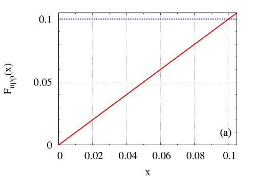
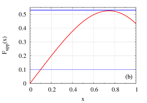
Figure 5: $F_{\mathrm{upp}}(x)$ (a) $0\leq x\leq 0.1$. (b) $0\leq x\leq 1$.

Proof of (30): We have the inequality between the ground-state energy $E_{\mathrm{Rabi}}$ and the lowest-energy sum $E_{\mathrm{les}}(\varepsilon)$ given in (28) as

$$E_{\mathrm{Rabi}} =\langle\psi_{\mathrm{Rabi}}|H_{\mathrm{Rabi}}|\psi_{\mathrm{Rabi}}\rangle$$

$$=\langle\psi_{\mathrm{Rabi}}|H_{\mathrm{JC}}^{\mathrm{g}}(\varepsilon)|\psi_{\mathrm{Rabi}}\rangle+\varepsilon\langle\psi_{\mathrm{Rabi}}|H_{\mathrm{JC}}^{\mathrm{g}/\varepsilon}(0)|\psi_{\mathrm{Rabi}}\rangle$$

$$\geq E_{\mathrm{JC}}^{\mathrm{g}}(\varepsilon)+\varepsilon E_{\mathrm{JC}}^{\mathrm{g}/\varepsilon}(0)\equiv E_{\mathrm{les}}(\varepsilon).$$

Here we used the decomposition (19). So, we realize by this inequality that the non-commutative energy $E_{\mathrm{diff}}(\varepsilon)$ is non-negative because of its definition, $E_{\mathrm{diff}}(\varepsilon)\equiv E_{\mathrm{Rabi}}-E_{\mathrm{les}}(\varepsilon)$. Thus, combining the inequalities (36) and (81), we reach the inequality:

$$0\leq E_{\mathrm{diff}}(\varepsilon)\leq E_{\mathrm{ubd}}^{\mathrm{g}}(\varepsilon)\leq\hbar\omega\Bigl{[}\frac{1}{2}-\varepsilon\left(|\nu_{**}|-|\nu_{*}|+1\right)\Bigr{]},$$

which implies (30).

C.5 Proofs of (27) and (52)

We define the subspace $\mathcal{H}_{+}$ by the space consisting of all superpositions of the states $|n,\uparrow\rangle$ and $|n+1,\downarrow\rangle$ for all even numbers $n$. Similarly, we give the subspace $\mathcal{H}_{-}$ by the space consisting of all superpositions of the states $|0,\downarrow\rangle$, $|n,\uparrow\rangle$, and $|n+1,\downarrow\rangle$ for all odd numbers $n$. Then, we realize that $\Pi\psi=(\sharp 1)\psi$ for wave functions $\psi\in\mathcal{H}_{\sharp}$, where $\Pi$ was the parity operator $\sigma_{z}(-1)^{a^{\dagger}a}$. We know that the ground state of the Rabi Hamiltonian is continuous with respect to the coupling strength $\mathrm{g}$. For instance, we can see it using the representation $H_{\mathrm{Rabi}}=H_{\mathrm{asym}}+(\hbar\omega/2)\sigma_{z}$ with the expression (10), together with the facts that the asymptotic Hamiltonian $H_{\mathrm{asym}}$ is solvable and that the ground state of the Rabi Hamiltonian is unique for every coupling strength $\mathrm{g}$ [26]. In addition to this continuity, the Rabi Hamiltonian has the parity symmetry Eq.(64). So, the normalized ground state $\varphi_{\mathrm{Rabi}}$ belongs to the subspace $\mathcal{H}_{-}$:

(i) $\varphi_{\mathrm{Rabi}}\in\mathcal{H}_{-}$, since it belongs to that subspace as $\mathrm{g}=0$: $\varphi_{\mathrm{Rabi}}(\mathrm{g}=0)=|0,\downarrow\rangle\in\mathcal{H}_{-}$.

Meanwhile, the eigenstates $\{\varphi_{\nu}^{\mathrm{g}}(\varepsilon)\}_{\nu\in\mathbb{Z}}$ (resp. $\{\varphi_{\nu}^{\mathrm{g}/\varepsilon}(0)\}_{\nu\in\mathbb{Z}}$) of the parameterized JC Hamiltonian $H_{\mathrm{JC}}^{\mathrm{g}}(\varepsilon)$ (resp. $H_{\mathrm{JC}}^{\mathrm{g}/\varepsilon}(0)$) makes a complete orthonormal basis of our state space. Moreover, we have the relations:

(ii) $\varphi_{0}^{\mathrm{g}}(\varepsilon),\varphi_{0}^{\mathrm{g}/\varepsilon}(0)\in\mathcal{H}_{-}$;

(iii) $\varphi_{\pm|\nu|}^{\mathrm{g}}(\varepsilon),\varphi_{\pm|\nu|}^{\mathrm{g}/\varepsilon}(0)\in\mathcal{H}_{-}$ if $n=|\nu|-1$ is odd (i.e., $|\nu|$ is even);

(iv) $\varphi_{\pm|\nu|}^{\mathrm{g}}(\varepsilon),\varphi_{\pm|\nu|}^{\mathrm{g}/\varepsilon}(0)\in\mathcal{H}_{+}$ if $n=|\nu|-1$ is even (i.e., $|\nu|$ is odd).

The ground state of the Rabi Hamiltonian is expressed using its normalized ground state $\varphi_{\mathrm{Rabi}}$ as $E_{\mathrm{Rabi}}=\langle\varphi_{\mathrm{Rabi}}|H_{\mathrm{Rabi}}|\varphi_{\mathrm{Rabi}}\rangle$. Applying the chiral decomposition (19) to this, we have the equation

$$E_{\mathrm{Rabi}}=\langle\varphi_{\mathrm{Rabi}}|H_{\mathrm{JC}}^{\mathrm{g}}(\varepsilon)|\varphi_{\mathrm{Rabi}}\rangle+\varepsilon\langle\sigma_{x}\varphi_{\mathrm{Rabi}}|H_{\mathrm{JC}}^{\mathrm{g}/\varepsilon}(0)|\sigma_{x}\varphi_{\mathrm{Rabi}}\rangle.$$

Inserting the expansion of $\varphi_{\mathrm{Rabi}}$ by $\varphi_{\nu}^{\mathrm{g}}(\varepsilon)$ and the expansion of $\sigma_{x}\varphi_{\mathrm{Rabi}}$ by $\varphi_{\nu}^{\mathrm{g}/\varepsilon}(0)$, respectively, into the LHS of the individual inner products, we reach the expansion,

$$E_{\mathrm{Rabi}}=\sum_{\nu\in\mathbb{Z}}\left[E_{\nu}^{\mathrm{g}}(\varepsilon)|\langle\varphi_{\nu}^{\mathrm{g}}(\varepsilon)|\varphi_{\mathrm{Rabi}}\rangle|^{2}+\varepsilon E_{\nu}^{\mathrm{g}/\varepsilon}(0)|\langle\varphi_{\nu}^{\mathrm{g}/\varepsilon}(0)|\sigma_{x}\varphi_{\mathrm{Rabi}}\rangle|^{2}\right].$$

We can derive Eq.(27) from this because the above properties (i)–(iv) concerning parity-symmetry and the fact $\sigma_{x}\varphi_{\mathrm{Rabi}}\in\mathcal{H}_{+}$ imply

$$A_{\nu}=\langle\varphi_{\nu}^{\mathrm{g}}(\varepsilon)|\varphi_{\mathrm{Rabi}}\rangle=0\,\,\,\,\,\text{if $|\nu|$ is odd},$$

$$B_{\nu}=\langle\varphi_{\nu}^{\mathrm{g}/\varepsilon}(0)|\sigma_{x}\varphi_{\mathrm{Rabi}}\rangle=0\,\,\,\,\,\text{if $|\nu|$ is even}.$$ (82)

We define the orthogonal projection operator $P_{n}$ by $P_{n}:=|n\rangle\langle n|$. Then, we have the expression of the number operator $N:=a^{\dagger}a$ as $N=\sum_{n=0}^{\infty}nP_{n}=\sum_{n=1}^{\infty}nP_{n}$, and thus, we have the equation $P_{0}+N=P_{0}+\sum_{n=1}^{\infty}nP_{n}$, which implies the operator inequality $P_{0}+N\geq\sum_{n=0}^{\infty}P_{n}=1$. Thus, we reach the operator inequality:

$$P_{0}\geq 1-N.$$ (83)

In the same way as in Lemma 4.3 of Ref.[39], we have the inequality:

$$\langle\varphi_{\mathrm{Rabi}}|N|\varphi_{\mathrm{Rabi}}\rangle\leq\frac{\mathrm{g}^{2}}{\omega^{2}},$$ (84)

where $\varphi_{\mathrm{Rabi}}$ is the normalized ground state with the ground-state energy $E_{\mathrm{Rabi}}$ of the Rabi Hamiltonian. Precisely, this is proved as follows: Using the commutator $[H_{\mathrm{Rabi}},a]\varphi_{\mathrm{Rabi}}=(H_{\mathrm{Rabi}}-E_{\mathrm{Rabi}})a\varphi_{\mathrm{Rabi}}$ with $[H_{\mathrm{Rabi}},a]=\,-\hbar\omega a-\hbar\mathrm{g}\sigma_{x}$, we reach the so-called pull-through formula,

$$a\varphi_{\mathrm{Rabi}}=\,-\hbar\mathrm{g}(H_{\mathrm{Rabi}}-E_{\mathrm{Rabi}}+\hbar\omega)^{-1}\sigma_{x}\varphi_{\mathrm{Rabi}}.$$

Applying this pull-through formula to the term $\langle\varphi_{\mathrm{Rabi}}|N|\varphi_{\mathrm{Rabi}}\rangle$ and using the Schwarz inequality, we obtain the inequality (84).

The two inequalities (83) and (84) imply the lower bound:

$$\langle\varphi_{\mathrm{Rabi}}|P_{0}|\varphi_{\mathrm{Rabi}}\rangle\geq 1-\frac{\mathrm{g}^{2}}{\omega^{2}}.$$ (85)

Meanwhile, the Schwarz inequality brings the upper bound:

$$\langle\varphi_{\mathrm{Rabi}}|P_{0}|\varphi_{\mathrm{Rabi}}\rangle\leq\|\varphi_{\mathrm{Rabi}}\|\,\|P_{0}\varphi_{\mathrm{Rabi}}\|\leq\|\varphi_{\mathrm{Rabi}}\|^{2}=1.$$ (86)

Since the equation $|A_{0}|^{2}+|B_{0}|^{2}=\langle\varphi_{\mathrm{Rabi}}|P_{0}|\varphi_{\mathrm{Rabi}}\rangle$ follows from the straightforward computation, we eventually obtain our desired estimate (52) by Eq.(82), the bounds (85) and (86).

References

- [1] E. Witten, Dynamical breaking of supersymmetry, Nucl. Phys. B 188, 513 (1981); Constraints on supersymmetry breaking, Nucl. Phys. B 202, 253 (1982).
- [2] P. Salomonson and J. W. Holten, Fermionic coordinates and supersymmetry in quantum mechanics, Nucl. Phys. B 196, 509 (1982).
- [3] M. de Crombrugghe and V. Rittenberg, Supersymmetric quantum mechanics, Ann. Phys. (NY) 151, 99 (1983).
- [4] M. Claudson and M. Halpern, Supersymmetric ground state wave functions, Nucl. Phys. B 250, 689 (1985).
- [5] E. D’Hoker and L. Vinet, Spectrum (super-)symmetries of particles in a Coulomb potential, Nucl. Phys. B 260, 79 (1985).
- [6] A. B. Balantekin, Accidental degeneracies and supersymmetric quantum mechanics, Ann. Phys. (NY) 164, 277 (1985).
- [7] J. C. D’Olivo, L. F. Urrutia, and F. Zertuche, Study of a three-dimensional quantum-mechanical supersymmetric model with nucleon-nucleon-type interaction, Phys. Rev. D 32, 2174 (1985).
- [8] A. Jaffe, A. Lesniewski, and M. Lewenstein, Ground state structure in supersymmetric quantum mechanics, Ann. Phys. (NY) 178, 313 (1987).
- [9] A. Arai, Supersymmetric embedding of a model of a quantum harmonic oscillator interacting with infinitely many bosons, J. Math. Phys. 30, 512 (1989).
- [10] B. F. Samsonov and V. V. Shamshutdinova, Dynamical qubit controlling via psedudo-supersymmetry of two-level systems, J. Phys. A 41, 244023 (2008).
- [11] A. Gangopadhyaya, J. V. Mallow, and C. Rasinariu, Supersymmetric Quantum Mechanics, World Scientific, 2011.
- [12] F. Schwabl, Quantum Mechanics, Springer, 2007.
- [13] T. Kuroki and F. Sugino, Spontaneous supersymmetry breaking by large- matrices, Nucl. Phys. B 796, 471 (2008); Spontaneous supersymmetry breaking in large- matrix models with slowly varying potential, Nucl. Phys. B 830, 434 (2010); Spontaneous supersymmetry breaking in matrix models from the viewpoints of localization and Nicolai mapping, Nucl. Phys. B 844, 409 (2011).
- [14] S. Haroche, J. M. Raimond, Exploring Quantum. Atoms, Cavities, and Photons, (Oxford University Press, 2008).
- [15] J. M. Raimond, M. Brune, S. Harohe, Manipulating quantum entanglement with atoms and photons in a cavity, Rev. Mod. Phys. 73, 565 (2001).
- [16] F. Marquardt and C. Bruder, Superposition of two mesoscopically distinct quantum states: Coupling a Cooper-pair box to a large superconducting island, Phys. Rev. B 63, 054514 (2001); Yu. Makhilin, G. Schön, A. Shnirman, Quantum-state engineering with Josephson-junction devices, Rev. Mod. Phys. 73, 357 (2001).
- [17] A. Blais, R.-S. Huang, S. Givrin, and R. Schoelkopf, Cavity quantum electrodynamics for superconducting electrical circuits: An architecture for quantum computation, Phys. Rev. A 69, 062320 (2004).
- [18] I. Chiorescu, P. Bertet, K. Semba, Y. Nakamura, C. J. P. M. Harmans, and J. E. Mooij, Coherent dynamics of a flux qubit coupled to a harmonic oscillator, Nature 431, 159 (2004); A. Wallraff, D. I. Schuster, A. Blais, L. Fruzio, R.-S. Huang, J. Majer, S. Kuar, S. M. Girvin, R. J. Schoelkopf, Strong coupling of a single photon to a superconducting qubit using circuit quantum electrodynamics, Nature 431, 162 (2004).
- [19] J. M. Fink, M. Göppl, M. Baur, R. Bianchetti, P. J. Leek, A. Blais, and A. Wallraff, Climbing the Jaynes–Cummings ladder and observing its nonlinearity in a cavity QED system, Nature 454, 315 (2008).
- [20] T. Niemczyk, F. Deppe, H. Huebl, E. P. Menzel, F. Hocke, M. J.Schwarz, J. J. Garcia-Ripoll, D. Zueco, T. Hümmer, E. Solano, A. Marx, and R. Gross, Circuit quantum electrodynamics in the ultrastrong-coupling regime, Nature Physics 6, 772 (2010); P. Forn-Díaz, J. Lisenfeld, D. Marcos, J. J. García-Ripoll, E. Solano, C. J. P. M. Harmans, and J. E. Mooij, Observation of the Bloch-Siegert Shift in a Qubit-Oscillator System in the Ultrastrong Coupling Regime, Phys. Rev. Lett. 105, 237001 (2010).
- [21] F. Hund, Zur Deutung der Molekelspektren. I, Z. Phys. 40, 742, (1927); Zur Deutung der Molekelspektren. II, Z. Phys. 42, 93, (1927); Zur Deutung der Molekelspektren. III, Z. Phys. 43, 805, (1927).
- [22] A. S. Wightman and N. Glance, Superselection rules in molecules, Nuclear Physics B (Proc. Suppl.) 6, 202, (1989); A. S. Wightman, Superselection rules; old and new, Nuovo Cimento B 110, 751, (1995).
- [23] A. Bermudez, M. A. Martin-Delgado, and E. Solano, Mesoscopic Superposition States in Relativistic Landau Levels, Phys. Rev. Lett. 99, 123602 (2007); A. Bermudez, M. A. Martin-Delgado, and A. Luis, Chirality quantum phase transition in the Dirac oscillator, Phys. Rev. A 77, 063815 (2008).
- [24] R. P. Feynman, Simulating Physics with Computers, Int. J. Theor. Phys. 21, 467 (1982).
- [25] D. Braak, Integrability of the Rabi Model, Phys. Rev. Lett. 107, 100401 (2011).
- [26] M. Hirokawa and F. Hiroshima, Absence of Energy Level Crossing for the Ground State Energy of the Rabi Model, arXiv:1207.4020.
- [27] H. G. Reik and M. Doucha, Exact Solution of the Rabi Hamiltonian by Known Functions? Phys. Rev. Lett. 57, 787 (1986).
- [28] M. Kuś, Statistical Properties of the Spectrum of the Two-Level System, Phys. Rev. Lett. 54, 13431 (1985).
- [29] H. A. Schmitt and A. Mufti, Two-level Jaynes-Cummings Hamiltonian as a supersymmetric quantum-mechanical system, Phys. Rev. D 43, 2743 (1991).
- [30] V. A. Kostelecky, M. M. Nieto, and D. R. Truax, Supersymmetry and the relationship between the Coulomb and oscillator problems in arbitrary dimensions, Phys. Rev. D 32, 2627 (1985).
- [31] M. Devoret, S. Girvin, and R. Schoelkopf, Circuit-QED: Howstrong can the coupling between a Josephson junction atom and a transmission line resonator be? Ann. Phys. (Leipzig) 16, 767 (2007).
- [32] J. Clarke and F. K. Wilhelm, Superconducting quantum bits, Nature 453, 1031 (2008); G. Günter, A. A. Anappara, J. Hees, A. Sell, G. Biasiol, L. Sorba, S. De Liberato, C. Ciuiti, A. Tredicucci, A. Leitenstorfer, adn R. Huber, Sub-cycle switch-on of ultrastrong light–matter interaction, Nature 458, 178 (2009).
- [33] J. Casanova, G. Romera, I. Lizuain, J. J. García-Ripoll, and E. Solano, Deep Strong Coupling Regime of the Jaynes-Cummings Model, Phys. Rev. Lett. 105, 263603 (2010).
- [34] A. D. Alhaidari, The supersymmetric Jaynes-Cummings model and its solution, J. Phys. A: Math. Gen. 39 (2006) 15391.
-
[35]
S.-J. Rey, “Quantum Phase Transition from String Theory”
at String 07, Madrid, June 25–29 (2007)
(http://www.ift.uam.es/strings07/040_scientific07_contents/videos/rey.mp4);
String Theory on Thin Semiconductors –Holographic Realization of Fermi Points and Surfaces–, Prog. Theo. Phys. Suppl. 177, 128 (2009). - [36] M. Hirokawa, The Dicke-Type Crossings among Eigenvalues of Differential Operators in A Class of Non-Commutative Oscillator, Indiana Univ. Math. J. 58, 1493 (2009).
- [37] M. Hirokawa, Dicke-type energy level crossings in cavity-induced atom cooling: Another superradiant cooling, Phys. Rev. A 79, 043408 (2009).
- [38] X. Peng, J. Zhang, J. Du, and D. Suter, Ground-state entanglement in a system with many-body interactions, Phys. Rev. A 81, 042327 (2010).
- [39] A. Arai and M. Hirokawa, On the Existence and Uniqueness of Ground States of a Generalized Spin-Boson Model, J. Funct. Anal. 151, 455 (1997).
-
[40]
K. Hepp and E. Lieb,
On the superradiant phase transition for molecules in a quantized radiation field: the dicke maser model,
Ann. Phys. 76, 360 (1973);
Equilibrium Statistical Mechanics of Matter Interacting with the Quantized Radiation Field, Phys. Rev. A 8, 2517 (1973). - [41] V. M. Bastidas, C. Emary, B. Regler, and T. Brandes, Nonequilibrium Quantum Phase Transitions in the Dicke Model Phys. Rev. Lett. 108, 043003 (2012).
- [42] M. Reed and B. Simon, Methods of Moderm Mathematical Physics I: Functional Analysis, (Academic Press, New York, 1980).
- [43] M. Hirokawa, An Expression of the Ground State Energy of the Spin-Boson Model, J. Funct. Anal. 162, 178 (1999).
- [44] A. Altland and B. Simons, Condensed Matter Field Theory, 2nd edition (Cambridge University Press, New York, 2010).