The Mean First Rotation Time of a planar polymer

Abstract

We estimate the mean first time, called the mean rotation time (MRT), for a planar random polymer to wind around a point. This polymer is modeled as a collection of $n$ rods, each of them being parameterized by a Brownian angle. We are led to study the sum of i.i.d. imaginary exponentials with one dimensional Brownian motions as arguments. We find that the free end of the polymer satisfies a novel stochastic equation with a nonlinear time function. Finally, we obtain an asymptotic formula for the MRT, whose leading order term depends on $\sqrt{n}$ and, interestingly, depends weakly on the mean initial configuration. Our analytical results are confirmed by Brownian simulations.

1 Introduction

This paper focusses mainly on some properties of a planar polymer motion and in particular, on the mean time that a rotation is completed around a fixed point. This mean rotation time (MRT) provides a quantification for the transition between a free two dimensional Brownian motion and a restricted motion. To study the distribution of this time, we shall use a simplified model of a polymer made of a collection of $n$ two dimensional connected rods with Brownian random angles (Figure 1). To estimate the mean rotation time, we shall fix one end of the polymer. We shall examine how the MRT depends on various parameters such as the diffusion constant, the number of rods or their common length. Using some approximations and numerical simulations, the mean time for the two polymer ends to meet was estimated in dimension three [WiF74, PZS96].

Although the windings of a (planar) Brownian motion, that is the number of rotations around one point in dimension 2 or a line in dimension three and its asymptotic behavior have been studied quite extensively [Spi58, PiY86, LeGY87, LeG90, ReY99], little seems to be known about the mean time for a rotation to be completed for the first time. For an Ornstein-Uhlenbeck process, the first time that it hits the boundary of a given cone was recently estimated [Vak10].

The paper is organized as follows: in section 2, we present the polymer model. In section 3, we study a sum of i.i.d. exponentials of one dimensional Brownian motions. Interestingly, using a Central Limit Theorem, we obtain a new stochastic equation for the limit process. This equation describes the motion of the free polymer end. In section 4, we obtain our main result which is an asymptotic formula for $E\left[\tau_{n}\right]$ the MRT when the polymer is made of $n$ rods of equal lengths $l_{0}$ with the first end fixed at a distance $L$ from the origin and the Brownian motion is characterized by its rotational diffusion constant $D$. We find that the MRT depends logarithmically on the mean initial configuration and for $nl_{0}>>L$ and $n\geq 3$, the leading order term is given by:

1. for a general initial configuration:

   $$E\left[\tau_{n}\right]\approx\frac{\sqrt{n}}{8D}\left[2\ln\left(\frac{E\left(\sum^{n}_{k=1}e^{\frac{i}{\sqrt{2D}}\theta_{k}(0)}\right)}{\sqrt{n}}\right)+Q\right],$$

   where $\left(\theta_{k}(0),1\leq k\leq n\right)$ are the initial angles of the polymer and $Q\approx 9.56$,

2. for an initially stretched polymer:

   $$E\left[\tau_{n}\right]\approx\frac{\sqrt{n}}{8D}\;\left(\ln(n)+Q\right),$$

   
   

3. for an average over uniformly distributed initial angles:

   $$E\left[\tau_{n}\right]\approx\frac{\sqrt{n}}{8D}\;\tilde{Q},$$

   where $\tilde{Q}\approx 9.62$.

We confirm our analytical results with generic Brownian simulations with normalized parameters . Finally, in section 5 we discuss some related open questions.

2 Stochastic modeling of a planar polymer

Various models are available to study polymers: the Rouse model consists of a collection of beads connected by springs, while more sophisticated models account for bending, torsion and specific mechanical properties [Rou53, SSS80, DoE94]. Here, we consider a very crude approximation where a planar polymer is modeled as a collection of $n$ rigid rods, with equal fixed lengths $l_{0}$ and we denote their extremities by $\left(X_{0},X_{1},X_{2},\ldots,X_{n}\right)$ (Figure 1) in a framework with origin ${\bf 0}$. We shall fix one of the polymer ends $X_{0}=(L,0)$ (where $L>0$) on the $x$-axis.

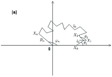
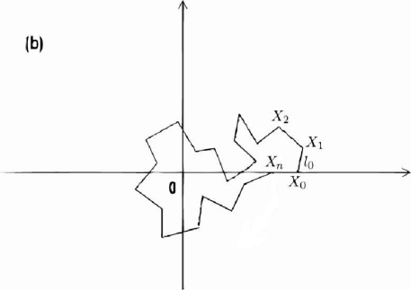
Figure 1: Schematic representation of a planar polymer winding around the origin.(a) A random configuration, (b) MRT when the $n$-th bead reaches $2\pi$.

The dynamics of the $i$-th rod is characterized by its angle $\theta_{i}(t)$ with respect to the $x$-axis. The overall polymer dynamics is thus characterized by the angles $\left(\theta_{1}(t),\theta_{2}(t),\ldots,\theta_{n}(t),t\geq 0\right)$. Due to the thermal collisions in the medium, each angle follows a Brownian motion. Thus, with $\stackrel{{\scriptstyle(law)}}{{=}}$ denoting equality in law,

$$\left(\theta_{i}(t),i\leq n\right)\stackrel{{\scriptstyle(law)}}{{=}}\sqrt{2D}\left(B_{i}(t),i\leq n\right)\ \mathrm{that}\ \mathrm{is:}\ \ d\theta_{i}(t)=\sqrt{2D}\>dB_{i}(t),\ \ i\leq n,$$

where $D$ is the rotational diffusion constant and $\left(B_{1}(t),\ldots,B_{n}(t),t\geq 0\right)$ is an $n$-dimensional Brownian motion (BM). The position of each rod can now be obtained as:

$$X_{1}(t)=L+l_{0}e^{i\theta_{1}(t)},\ X_{2}(t)=X_{1}(t)+l_{0}e^{i\theta_{2}(t)},\ \ldots,\ X_{n}(t)=X_{n-1}(t)+l_{0}e^{i\theta_{n}(t)}.$$

In particular, the moving end is given by:

$$X_{n}(t)=L+l_{0}\sum^{n}_{k=1}e^{i\theta_{k}(t)}=L+l_{0}\sum^{n}_{k=1}e^{i\sqrt{2D}B_{k}(t)},$$

which can be written as:

$$X_{n}(t)=R_{n}(t)e^{i\varphi_{n}(t)}.$$ (3)

Thus $\varphi_{n}(t)$ accounts for the rotation of the polymer with respect to the origin ${\bf 0}$ and $R_{n}$ is the distance to the origin.

In order to compute the MRT, we shall study a sum of exponentials of Brownian motions, a topic which often leads to surprising computations [Yor01]. First, we scale the space and time variables as follows:

$$\tilde{l}=\frac{L}{l_{0}}\ \ \mathrm{and}\ \ \tilde{t}=\frac{t}{2D}.$$ (4)

Equation (2) becomes:

$$X_{n}(t)=\tilde{l}+\sum^{n}_{k=1}e^{i\tilde{B}_{k}(t)},$$ (5)

where $\left(\tilde{B}_{1}(t),\ldots,\tilde{B}_{n}(t),t\geq 0\right)$ is an $n$-dimensional Brownian motion (BM), and for $k=1,\ldots,n$, using the scaling property of Brownian motion, we have:

$$\tilde{B}_{k}(t)\equiv\frac{1}{\sqrt{2D}}B_{k}(t)\stackrel{{\scriptstyle(law)}}{{=}}B_{k}\left(\frac{t}{2D}\right)=B_{k}(\tilde{t}).$$

Before describing our approach, we first discuss the mean initial configuration of the polymer. It is given by:

$$c_{n}=E\left(\sum^{n}_{k=1}e^{i\theta_{k}(0)}\right),$$ (6)

where the initial angles $\theta_{k}(0)$ are such that the polymer has not already made a loop. After scaling, the mean initial configuration becomes:

$$c_{n}=E\left(\sum^{n}_{k=1}e^{i\>\tilde{\theta}_{k}(0)}\right),$$ (7)

with

$$\tilde{\theta}_{k}(0)=\tilde{B}_{k}(0).$$ (8)

From now on, we use $\theta_{k}$ instead of $\tilde{\theta}_{k}$, $B$ instead of $\tilde{B}$ and $t$ instead of $\tilde{t}$. Any segment in the interior of the polymer can hit the angle $2\pi$ around the origin, but we will not consider this as a winding event, although we could and in that case, the MRT would be different. Rather, we shall only consider that, given an initial configuration $c_{n}$, the MRT is defined as:

$$MRT\equiv E\{\tau_{n}|c_{n}\}\equiv E\left[\tau_{n}\right],$$ (9)

where

$$\tau_{n}\equiv\inf\{t>0,|\varphi_{n}(t)|=2\pi\}.$$ (10)

Thus, an initial configuration is not winding when

$$\left|\varphi_{n}(0)\right|<2\pi.$$ (11)

Then, we can define the winding event using a one dimensional variable only. In general, winding is a rare event and we expect that the MRT will depend crucially on the length of the polymer which will be quite long. Interestingly, the rotation is accomplished when the angle $\varphi_{n}(t)$ reaches $2\pi$ or $-2\pi$, but the distance of the free end point to the origin is not fixed, leading to a one dimensional free parameter space. This undefined position is in favor of a winding time that is not too large when compared to any narrow escape problem where a Brownian particle has to find a small target in a confined domain [WaK93, HoS04, SSHE06, SSH07, BKH07, PWPSK09].

In this study, we consider not only that the initial condition satisfies $\left|\varphi_{n}(0)\right|<2\pi$, but we impose that $\varphi_{n}(0)$ is located far enough from $2\pi$, to avoid studying any boundary layer effect, which would lead to a different MRT law. Indeed, starting inside the boundary layer for a narrow escape type problem leads to specific escape laws [SSHE06]. Given a small $\varepsilon>0$ we shall consider the space of configurations $\Omega_{\varepsilon}$ such that $\left|\varphi_{n}(0)\right|<2\pi-\varepsilon$. We shall mainly focus on the stretched polymer,

$$\left(\theta_{1}(0),\theta_{2}(0),\ldots,\theta_{n}(0)\right)=\left(0,0,\ldots,0\right),$$ (12)

and thus $c_{n}=n>0$ (in this case, $\varphi_{n}(0)=0$). Finally, it is quite obvious that winding occurs only when the condition:

$$nl_{0}>L$$ (13)

is satisfied, which we assume all along.

The outline of our method is: first we show that the sum $X_{n}(t)$ converges (eq. (2)) and we obtain a Central Limit Theorem. Using Itô calculus, we study the sequence:

$$\frac{1}{\sqrt{n}}\overline{X}_{n}(t)=\frac{1}{\sqrt{n}}\left[X_{n}(t)-E\left(X_{n}(t)\right)\right].$$ (14)

and prove that $\frac{1}{\sqrt{n}}\overline{X}_{n}(t)$, for $n$ large, converges to a stochastic process which is a generalization of an Ornstein-Uhlenbeck process (GOUP), containing a time dependent deterministic drift $c_{n}e^{-t}$. This GOUP is driven by a martingale $\left(M_{t}^{(n)},t\geq 0\right)$ that we further characterize. Interestingly, the two cartesian coordinates of $\left(M_{t}^{(n)},t\geq 0\right)$ converge to two independent Brownian motions with two different time scale functions. To obtain an asymptotic formula for the MRT, we show that in the long time asymptotics, where winding occurs, the GOUP can be approximated by a standard Ornstein-Uhlenbeck process (OUP). Using some properties of the GOUP [Vak10], we finally derive the MRT for the polymer which is the mean time that $|\varphi_{n}(t)|=2\pi$.

3 Properties of the free polymer end $X_{n}(t)$ using a Central Limit Theorem

In this section we study some properties of the free polymer end $X_{n}(t)$. In particular, using a Central Limit Theorem, we show that the limit process satisfies a stochastic equation of a new type. To study the random part of $X_{n}(t)$, we shall remove from it its first moment and we shall now consider the asymptotic behavior of the drift-less sequence:

$$\frac{1}{\sqrt{n}}\overline{X}_{n}(t)=\frac{1}{\sqrt{n}}\left[X_{n}(t)-E\left(X_{n}(t)\right)\right].$$ (15)

We start by computing the first moment $E\left(X_{n}(t)\right)$. Because (see (2)), $\left(\theta_{i}(t),t\geq 0\right)$ are assumed to be $n$ independent identically distributed (iid) Brownian motions with variance $2D$, after rescaling, we obtain:

$$E\left(X_{n}(t)\right) = E\left[\tilde{l}+\sum^{n}_{k=1}e^{iB_{k}(t)}\right]$$ (16)

$$= \tilde{l}+\left(\sum^{n}_{k=1}E\left[e^{i\left(B_{k}(t)-B_{k}(0)\right)}\right]\>E\left[e^{i\left(B_{k}(0)\right)}\right]\right)$$

$$= \tilde{l}+c_{n}e^{-\frac{t}{2}}.$$

where $c_{n}$ is defined by (7) and we have used that:

$$E\left[e^{i\left(B_{k}(t)-B_{k}(0)\right)}\right]=e^{-\frac{t}{2}}\ .$$ (17)

We study the sequence (15) as follows:

$$\frac{1}{\sqrt{n}}\overline{X}_{n}(t) = \frac{1}{\sqrt{n}}\left[\sum^{n}_{k=1}e^{iB_{k}(t)}-E\left(\sum^{n}_{k=1}e^{iB_{k}(t)}\right)\right]$$ (18)

$$= \frac{1}{\sqrt{n}}\sum^{n}_{k=1}F_{k}(t),$$

where $F_{k}(t)=e^{iB_{k}(t)}-E\left(e^{iB_{k}(t)}\right)$. Applying Itô’s formula to

$$Z_{t}^{(n)}=\frac{1}{\sqrt{n}}\sum^{n}_{k=1}F_{k}(t)\ ,$$ (19)

with $Z_{0}^{(n)}=0$, we obtain:

$$Z_{t}^{(n)} = \frac{i}{\sqrt{n}}\int^{t}_{0}\sum^{n}_{k=1}e^{iB_{k}(s)}dB_{k}(s)-\frac{1}{2\sqrt{n}}\int^{t}_{0}\sum^{n}_{k=1}\left(e^{iB_{k}(s)}-E\left(e^{iB_{k}(s)}\right)\right)ds$$ (20)

$$= M_{t}^{(n)}-\frac{1}{2}\int^{t}_{0}Z_{s}^{(n)}\>ds,$$

where:

$$M_{t}^{(n)} = \frac{i}{\sqrt{n}}\int^{t}_{0}\sum^{n}_{k=1}e^{iB_{k}(s)}\>dB_{k}(s)$$ (21)

$$= \frac{1}{\sqrt{n}}\int^{t}_{0}\sum^{n}_{k=1}\left(i\cos(B_{k}(s))-\sin(B_{k}(s))\right)\>dB_{k}(s)$$

$$= -S_{t}^{(n)}+iC_{t}^{(n)}.$$

We shall now study the asymptotic limit of the martingales $M_{t}^{(n)}$ as $n\rightarrow\infty$ and summarize our result in the following theorem; the convergence in law being considered there is associated with the topology of the uniform convergence on compact sets of the functions in $C(\mathbb{R}_{+},\mathbb{R}^{2})$.

Theorem 3.1

The sequence $(M_{t}^{(n)},t\geq 0)$ converges in law to a Brownian motion in dimension 2, with 2 deterministic time changes. More precisely,

$$(S^{(n)}_{t},C^{(n)}_{t},t\geq 0)\overset{{(law)}}{\underset{n\rightarrow\infty}{\longrightarrow}}(\sigma_{\left(\frac{1}{2}\int^{t}_{0}ds\>(1-e^{-2s})\right)},\gamma_{\left(\frac{1}{2}\int^{t}_{0}ds\>(1+e^{-2s})\right)},t\geq 0),$$ (22)

where $(\sigma_{u},\gamma_{u},u\geq 0)$ are two independent Brownian motions.

Remark 3.2

$\left.a\right)$ The convergence in law (22) is a new result and it shows that the sum of the complex exponentials of i.i.d. Brownian motions can be approximated by a two dimensional Brownian motion, with a different time scale for each coordinate.
$\left.b\right)$ An extension of Theorem 3.1 when $\left(\exp\left(iB(s)\right),s\geq 0\right)$ a Brownian motion on the unit circle is replaced by a BM on the unit sphere in $\mathbb{R}^{n}$ is obtained in [HVY11].

Proof of Theorem 3.1 See Appendix A.     

We conclude that the sequence $(M_{t}^{(n)},t\geq 0)$ converges in law:

$$(M_{t}^{(n)},t\geq 0)\overset{{(law)}}{\underset{n\rightarrow\infty}{\longrightarrow}}(\sigma_{\left(\frac{t}{2}-\frac{1-e^{-2t}}{4}\right)}+i\gamma_{\left(\frac{t}{2}+\frac{1-e^{-2t}}{4}\right)},t\geq 0).$$ (23)

The process $(Z_{t}^{(n)},t\geq 0)$, which we defined in (20), is a generalization of the classical Ornstein-Uhlenbeck process; it is driven by $(M_{t}^{(n)},t\geq 0)$ and, from (20), we obtain:

$$Z_{t}^{(n)} = e^{-\frac{t}{2}}\int^{t}_{0}e^{\frac{s}{2}}dM_{s}^{(n)}.$$ (24)

Corollary 3.3

$\left.\mathrm{a}\right)$ The sequence $(Z_{t}^{(n)},t\geq 0)$ converges in law:

$$Z_{t}^{(n)}\overset{{(law)}}{\underset{n\rightarrow\infty}{\longrightarrow}}Z_{t}^{(\infty)},$$ (25)

with:

$$Z_{t}^{(\infty)}=e^{-\frac{t}{2}}\int^{t}_{0}\sqrt{\sinh(s)}\;d\delta_{s}+i\;e^{-\frac{t}{2}}\int^{t}_{0}\sqrt{\cosh(s)}\;d\tilde{\delta}_{s},$$ (26)

where $\left(\delta_{t},\tilde{\delta}_{t},t\geq 0\right)$ are two independent 1-dimensional Brownian motions. $\left.\mathrm{b}\right)$ $Z_{t}^{(\infty)}\overset{{(law)}}{\underset{t\rightarrow\infty}{\longrightarrow}}\frac{1}{\sqrt{2}}\left(N+i\tilde{N}\right)$, where $N$ and $\tilde{N}$ are two centered and reduced Gaussian variables.

Proof of Corollary 3.3
$\left.\mathrm{a}\right)$ From (21), (22) and (24) we deduce:

$$Z_{t}^{(n)} = e^{-\frac{t}{2}}\int^{t}_{0}e^{\frac{s}{2}}dM_{s}^{(n)}$$

$$\overset{{(law)}}{\underset{n\rightarrow\infty}{\longrightarrow}} e^{-\frac{t}{2}}\int^{t}_{0}\underbrace{e^{\frac{s}{2}}\sqrt{\frac{1-e^{-2s}}{2}}}_{\sqrt{\sinh(s)}}\;d\delta_{s}+ie^{-\frac{t}{2}}\int^{t}_{0}\underbrace{e^{\frac{s}{2}}\sqrt{\frac{1+e^{-2s}}{2}}}_{\sqrt{\cosh(s)}}\;d\tilde{\delta}_{s}\equiv Z_{t}^{(\infty)}.$$

$\left.\mathrm{b}\right)$ From (LABEL:2Zncvgfinal), we change variables: $u=t-s$ and we obtain:

$$Z_{t}^{(\infty)} = \int^{t}_{0}e^{-\frac{t-s}{2}}\sqrt{\frac{1-e^{-2s}}{2}}\;d\delta_{s}+i\int^{t}_{0}e^{-\frac{t-s}{2}}\sqrt{\frac{1+e^{-2s}}{2}}\;d\tilde{\delta}_{s}$$ (30)

$$\overset{{u=t-s}}{\underset{(law)}{=}} \int^{t}_{0}e^{-\frac{u}{2}}\sqrt{\frac{1}{2}-\frac{e^{-2(t-u)}}{2}}\;d\delta_{u}+i\int^{t}_{0}e^{-\frac{u}{2}}\sqrt{\frac{1}{2}+\frac{e^{-2(t-u)}}{2}}\;d\tilde{\delta}_{u}$$

$$\overset{{L^{2}}}{\underset{t\rightarrow\infty}{\longrightarrow}} \frac{1}{\sqrt{2}}\int^{\infty}_{0}e^{-\frac{u}{2}}d\delta_{u}+i\;\frac{1}{\sqrt{2}}\int^{\infty}_{0}e^{-\frac{u}{2}}d\tilde{\delta}_{u}\ ,$$

where the two variables on the RHS of (30) are centered Gaussian with variance $1/2$ and the convergence in $L^{2}$ for $t\rightarrow\infty$ may be proved by using the dominated convergence theorem.     

Remark 3.4

In [Itô83] and [Ochi85] there is a more complete asymptotic study for $Z_{t}^{(n)}(\varphi)$, as $n\rightarrow\infty$, for a large class of functions $\varphi$, but we do not pursue this line of research here.

On one hand, from the identities (15), (16), (18) and (19), we obtain the following expansion:

$$X_{n}(t) = \overline{X}_{n}(t)+E\left[X_{n}(t)\right]$$

$$= \sqrt{n}\>Z_{t}^{(n)}+c_{n}e^{-\frac{t}{2}}+\tilde{l}$$

$$\Rightarrow\tilde{X}_{n}(t) \equiv X_{n}(t)-\tilde{l}=\sqrt{n}\>Z_{t}^{(n)}+c_{n}e^{-\frac{t}{2}},$$ (31)

with $n$ the number of rods/beads, $Z_{t}^{(n)}$ a GOUP driven by $M_{t}^{(n)}$ which is given by (23), $c_{n}=E\left(\sum^{n}_{k=1}e^{i\theta_{k}(0)}\right)$ a constant depending on the mean initial configuration and $\tilde{l}=\frac{L}{l_{0}}$ the rescaled distance of the fixed end from the origin ${\bf 0}$ ($l_{0}$ is the fixed length of the rods).
On the other hand, with Corollary 3.3(a), we deduce that:

$$Z^{(n)}_{t} \equiv \frac{1}{\sqrt{n}}\overline{X}_{n}(t)\equiv\frac{1}{\sqrt{n}}\left[X_{n}(t)-E\left(X_{n}(t)\right)\right]$$ (32)

$$= \frac{1}{\sqrt{n}}\left[X_{n}(t)-c_{n}e^{-\frac{t}{2}}-\tilde{l}\right]$$

$$\overset{{(law)}}{\underset{n\rightarrow\infty}{\longrightarrow}} e^{-\frac{t}{2}}\int^{t}_{0}\sqrt{\sinh(s)}\;d\delta_{s}+i\;e^{-\frac{t}{2}}\int^{t}_{0}\sqrt{\cosh(s)}\;d\tilde{\delta}_{s}\equiv Z^{(\infty)}_{t}.$$

4 Asymptotic expression for the MRT

We now study more precisely the different time scales of the two Brownian motions in (23) and (32). We estimate $Z_{t}^{(\infty)}$ for $t$ large, the regime for which the rotation will be accomplished.
We introduce here the following notation: $\stackrel{{\scriptstyle L^{2}}}{{\approx}}$ denotes closeness in the $L^{2}-$norm: for two stochastic processes $(W^{(1)}_{t},t\geq 0)$ and $(W^{(2)}_{t},t\geq 0)$, the notation $W^{(1)}_{t}\stackrel{{\scriptstyle L^{2}}}{{\approx}}W^{(2)}_{t}$ means that ${\underset{t\rightarrow\infty}{\lim}}E\left[\left|W^{(1)}_{t}-W^{(2)}_{t}\right|^{2}\right]=0$.
We shall show that, with $\left(\mathbb{B}_{t}=\delta_{t}+i\tilde{\delta}_{t},t\geq 0\right)$ a 2-dimensional Brownian motion starting from $1$:

$$Z_{t}^{(\infty)} = e^{-\frac{t}{2}}\int^{t}_{0}\sqrt{\sinh(s)}\;d\delta_{s}+i\;e^{-\frac{t}{2}}\int^{t}_{0}\sqrt{\cosh(s)}\;d\tilde{\delta}_{s}$$ (33)

$$\stackrel{{\scriptstyle L^{2}}}{{\approx}} e^{-\frac{t}{2}}\int^{t}_{0}\frac{e^{\frac{s}{2}}}{\sqrt{2}}d\mathbb{B}_{s}.$$

For this, it suffices to use the expression (30) and the following Proposition, which reinforces the $\stackrel{{\scriptstyle L^{2}}}{{\approx}}$ result in (33).

Proposition 4.1

As $t\rightarrow\infty$, the Gaussian martingales

$$\left(\int^{t}_{0}\sqrt{\sinh(s)}\;d\delta_{s}-\int^{t}_{0}\frac{e^{s/2}}{\sqrt{2}}\;d\delta_{s},t\geq 0\right),$$

and

$$\left(\int^{t}_{0}\sqrt{\cosh(s)}\;d\tilde{\delta}_{s}-\int^{t}_{0}\frac{e^{s/2}}{\sqrt{2}}\;d\tilde{\delta}_{s},t\geq 0\right)$$

converge a.s. and in $L^{2}$. The limit variables are Gaussian with variances $\frac{\pi-3}{2}$ and $-1+2\sqrt{2}-2a_{s}(1)\approx 0,033$, where $a_{s}(x)\equiv\arg\sinh(x)\equiv\log(x+\sqrt{1+x^{2}}),\ x\in\mathbb{R}$, respectively.

Thus, by multiplying both processes by $e^{-\frac{t}{2}}$, we obtain (33).

Proof of Proposition 4.1 The Gaussian martingale $\int^{t}_{0}\left(\sqrt{\sinh(s)}-\frac{e^{s/2}}{\sqrt{2}}\right)\;d\delta_{s}$ has increasing process

$$\int^{t}_{0}\left(\sqrt{\sinh(s)}-\frac{e^{s/2}}{\sqrt{2}}\right)^{2}\;ds=\int^{t}_{0}\frac{e^{s}}{2}\left(\sqrt{1-e^{-2s}}-1\right)^{2}\;ds\ ,$$

which converges as $t\rightarrow\infty$. Hence, the limit variable $\int^{\infty}_{0}\left(\sqrt{\sinh(s)}-\frac{e^{s/2}}{\sqrt{2}}\right)\;d\delta_{s}$ is Gaussian, and its variance is given by (we change variables: $u=e^{-2s}$ and $B(a,b)$ denotes the Beta function with arguments $a$ and $b$):

$$\int^{\infty}_{0}\frac{ds\;e^{s}}{2}\left(\sqrt{1-e^{-2s}}-1\right)^{2}=\frac{1}{4}\int^{1}_{0}du\;u^{-3/2}\left(\sqrt{1-u}-1\right)^{2}$$

$$= \frac{1}{4}\left[\int^{1}_{0}du\;u^{-3/2}\left((1-u)-2\sqrt{1-u}+1\right)\right]$$

$$= \frac{1}{4}\left\{B\left(-\frac{1}{2},2\right)-2B\left(-\frac{1}{2},\frac{3}{2}\right)-2\right\}=\frac{\pi-3}{2}\ .$$

To be rigorous, the integral $\int^{1}_{0}du\;u^{-\alpha}\left(\sqrt{1-u}-1\right)^{2}$, which is well defined for $0<\alpha<1$, can be extended analytically for any complex $\alpha$ with $\mathrm{Re}(\alpha)<3$.
For the convergence of the second process, it suffices to replace $\sinh(s)$ by $\cosh(s)\equiv\frac{e^{s}}{2}(1+e^{-2s})$. The limit variable $\int^{\infty}_{0}\left(\sqrt{\cosh(s)}-\frac{e^{s/2}}{\sqrt{2}}\right)\;d\tilde{\delta}_{s}$ is also Gaussian, and, repeating the previous calculation, we easily compute its variance.     

Asymptotic expression for the MRT

For $t$ large, we derive an asymptotic value for the MRT. First, from (24) and (3):

$$\tilde{X}_{n}(t) = \sqrt{n}Z^{(n)}_{t}+c_{n}e^{-\frac{t}{2}}$$ (34)

$$= \sqrt{n}e^{-\frac{t}{2}}\left(\tilde{c}_{n}+\int^{t}_{0}e^{\frac{s}{2}}dM^{(n)}_{s}\right),$$

where, the sequence $\tilde{c}_{n}$ is:

$$\tilde{c}_{n}\equiv\frac{c_{n}}{\sqrt{n}},$$ (35)

$n$ is the number of rods/beads, and $c_{n}\equiv E\left(\sum^{n}_{k=1}e^{i\theta_{k}(0)}\right)$ is a constant depending on the mean initial configuration. Thus, from (3), (33), (34) and also using the scaling property of Brownian motion:

$$\tilde{X}_{n}(t)\overset{{(law)}}{\underset{n:large}{\approx}}\sqrt{n}Y_{t}^{(n)},$$ (36)

where

$$Y_{t}^{(n)}\equiv e^{-\frac{t}{2}}\left(\tilde{c}_{n}+\int^{t}_{0}e^{\frac{s}{2}}d\mathbb{B}_{s/2}\right).$$ (37)

Changing time and expression of the MRT

To express the MRT, we now apply deterministic time changes. To make our writing simple, we denote $Y_{t}$ for $Y_{t}^{(n)}$, and changing variables $u=\frac{s}{2}$ in (37), we obtain:

$$Y_{2t}=e^{-t}\left(\tilde{c}_{n}+\int^{t}_{0}e^{u}d\mathbb{B}_{u}\right).$$ (38)

Now, there is another BM $(\tilde{\mathbb{B}}_{t},t\geq 0)$, starting from $\tilde{c}_{n}$, such that:

$$Y_{2t}=e^{-t}\left(\tilde{\mathbb{B}}_{\alpha_{t}}\right),$$ (39)

where:

$$\alpha_{t}=\int^{t}_{0}e^{2s}ds=\frac{e^{2t}-1}{2},$$

hence:

$$\alpha^{-1}(t)=\frac{1}{2}\ln\left(1+2t\right).$$ (40)

Applying Itô’s formula to (39), we obtain:

$$dY_{2s}=-e^{-s}\tilde{\mathbb{B}}_{\alpha_{s}}ds+e^{-s}d\left(\tilde{\mathbb{B}}_{\alpha_{s}}\right).$$

We divide by $Y_{2s}$ and we obtain:

$$\frac{dY_{2s}}{Y_{2s}}=-ds+\frac{d\tilde{\mathbb{B}}_{\alpha_{s}}}{\tilde{\mathbb{B}}_{\alpha_{s}}}.$$

Thus:

$$\mathrm{Im}\left(\frac{dY_{2s}}{Y_{2s}}\right)=\mathrm{Im}\left(\frac{d\tilde{\mathbb{B}}_{\alpha_{s}}}{\tilde{\mathbb{B}}_{\alpha_{s}}}\right),$$

which means that, if we denote:

$$\theta^{Z}_{t}\equiv\mathrm{Im}(\int^{t}_{0}\frac{dZ_{s}}{Z_{s}}),t\geq 0,$$ (41)

the continuous winding process associated to a generic stochastic process $Z$, then:

$$\theta^{Y}_{2t}=\theta^{\tilde{\mathbb{B}}}_{\alpha_{t}}.$$

Thus, the first hitting times of the symmetric conic boundary of angle $c$

$$T^{|\theta^{Y}|}_{c}\equiv\inf\left\{t\geq 0:\left|\theta^{Y}_{t}\right|=c\right\},$$ (42)

and

$$T^{|\theta^{\tilde{\mathbb{B}}}|}_{c}\equiv\inf\left\{t\geq 0:\left|\theta^{\tilde{\mathbb{B}}}_{t}\right|=c\right\},$$ (43)

for an Ornstein-Uhlenbeck process $Y$ with parameter $\lambda=1$, and for a Brownian motion $\tilde{\mathbb{B}}$ respectively, with relation (40), satisfy:

$$2T^{|\theta^{Y}|}_{c}=\frac{1}{2}\ln\left(1+2T^{|\theta^{\tilde{\mathbb{B}}}|}_{c}\right).$$ (44)

Finally,

$$E\left[2T^{|\theta^{Y}|}_{c}\right] = \frac{1}{2}E\left[\ln\left(1+2T^{|\theta^{\tilde{\mathbb{B}}}|}_{c}\right)\right]$$ (45)

$$= \frac{\ln 2}{2}+\frac{1}{2}E\left[\ln\left(T^{|\theta^{\tilde{\mathbb{B}}}|}_{c}+\frac{1}{2}\right)\right],$$ (46)

and equivalently:

$$E\left[T^{|\theta^{Y}|}_{c}\right] = \frac{\ln 2}{4}+\frac{1}{4}E\left[\ln\left(T^{|\theta^{\tilde{\mathbb{B}}}|}_{c}+\frac{1}{2}\right)\right].$$ (47)

Thus, by taking $c=2\pi$, for $n$ large, with $\tilde{\varphi}_{n}(t)$ denoting the total angle of $\tilde{X}_{n}(t)$, the mean time $E\left[\tilde{\tau}_{n}\right]$, where $\tilde{\tau}_{n}\equiv\inf\{t>0,|\tilde{\varphi}_{n}(t)|=2\pi\}$, that $\tilde{X}_{n}(t)$ rotates around ${\bf 0}$, is:

$$E\left[\tilde{\tau}_{n}\right] \approx \frac{\sqrt{n}}{4}\left(\ln 2+E\left[\ln\left(T^{|\theta^{\tilde{\mathbb{B}}}|}_{2\pi}+\frac{1}{2}\right)\right]\right).$$ (48)

By using the series expansion of $\log(1+x)$, we obtain informally:

$$E\left[\ln\left(T^{|\theta^{\tilde{\mathbb{B}}}|}_{c}+\frac{1}{2}\right)\right]-E\left[\ln\left(T^{|\theta^{\tilde{\mathbb{B}}}|}_{c}\right)\right] = E\left[\ln\left(1+\frac{1}{2T^{|\theta^{\tilde{\mathbb{B}}}|}_{c}}\right)\right]$$

$$= \frac{1}{2}E\left[\frac{1}{T^{|\theta^{\tilde{\mathbb{B}}}|}_{c}}\right]-\frac{1}{8}E\left[\left(\frac{1}{T^{|\theta^{\tilde{\mathbb{B}}}|}_{c}}\right)^{2}\right]+\ldots,$$

where this expansion should be understood as follows: we obtain an alternate series of negative moments of $T^{|\theta^{\tilde{\mathbb{B}}}|}_{c}$, which converges [VaY11]. For our purpose, we will truncate the series. We shall estimate and use only the first moment of $1/T^{|\theta^{\tilde{\mathbb{B}}}|}_{c}$. By numerical calculations, the other moments can be neglected.

From the skew product representation [KaSh88, ReY99] there is another planar Brownian motion $(\beta_{u}+i\gamma_{u},u\geq 0)$, starting from $\log\tilde{c}_{n}+i0$, such that:

$$\log\left|\tilde{\mathbb{B}}_{t}\right|+i\theta_{t}\equiv\int^{t}_{0}\frac{d\tilde{\mathbb{B}}_{s}}{\tilde{\mathbb{B}}_{s}}=\left(\beta_{u}+i\gamma_{u}\right)\Bigm{|}_{u=H_{t}\equiv\int^{t}_{0}\frac{ds}{\left|\tilde{\mathbb{B}}_{s}\right|^{2}}},$$ (51)

and equivalently:

$$\log\left|\tilde{\mathbb{B}}_{t}\right|=\beta_{H_{t}};\ \ \theta_{t}=\gamma_{H_{t}}.$$ (52)

Thus, with $T^{|\gamma|}_{c}\equiv\inf\left\{t\geq 0:\left|\gamma_{t}\right|=c\right\}$ and $T^{|\theta^{\tilde{\mathbb{B}}}|}_{c}\equiv\inf\left\{t\geq 0:\left|\theta^{\tilde{\mathbb{B}}}_{t}\right|=c\right\}$, because $\theta_{T^{|\theta^{\tilde{\mathbb{B}}}|}_{c}}=\gamma_{H_{T^{|\theta^{\tilde{\mathbb{B}}}|}_{c}}}$:

$$T^{|\gamma|}_{c}=H_{T^{|\theta^{\tilde{\mathbb{B}}}|}_{c}},$$

hence $T^{|\theta^{\tilde{\mathbb{B}}}|}_{c}=H^{-1}_{u}\Bigm{|}_{u=T^{|\gamma|}_{c}}$, where:

$$H^{-1}_{u}\equiv\inf\{t:H_{t}>u\}=\int^{u}_{0}ds\exp(2\beta_{s})\equiv A_{u},$$ (53)

and for $u=T^{|\gamma|}_{c}$, we obtain:

$$T^{|\theta^{\tilde{\mathbb{B}}}|}_{c}=A_{T^{|\gamma|}_{c}}.$$ (54)

It is of interest for our purpose to look at the first negative moment of $A_{t}$ which has the following integral representation for any $t>0$ ([Duf00], [D-MMY00], p.49, Prop. 7, formula (15)):

$$E\left[\frac{1}{A_{t}}\right]=\int^{\infty}_{0}ye^{-y^{2}t/2}\coth\left(\frac{\pi}{2}y\right)\;dy.$$ (55)

With $\beta_{s}=\log(\tilde{c}_{n})+\beta^{(0)}_{s}$, where $(\beta^{(0)}_{s},s\geq 0)$ is a one-dimensional Brownian motion starting from 0, we obtain:

$$T^{|\theta^{\tilde{\mathbb{B}}}|}_{c} = H^{-1}(T^{|\gamma|}_{c})\equiv\int^{T^{|\gamma|}_{c}}_{0}ds\;\exp\left(2\beta_{s}\right)$$ (56)

$$= (\tilde{c}_{n})^{2}\left(\int^{T^{|\gamma|}_{c}}_{0}ds\;\exp\left(2\beta^{(0)}_{s}\right)\right)$$

$$\equiv (\tilde{c}_{n})^{2}T^{|\theta^{\mathbb{B}^{(1)}}|}_{c}\ \ ,$$

where $T^{|\theta^{\mathbb{B}^{(1)}}|}_{c}\equiv\inf\left\{t\geq 0:\left|\theta^{\mathbb{B}^{(1)}}_{t}\right|=c\right\}$ is the first hitting time of the symmetric conic boundary of angle $c$ of a Brownian motion $\mathbb{B}^{(1)}$ starting from $1+i0$. Hence, from (54-55) and by using the Laplace transform for the hitting time $T^{|\gamma|}_{c}$ [ReY99] (Chapter II, Prop. 3.7) or [PiY03](p.298):

$$E\left[e^{-\frac{y^{2}}{2}T^{|\gamma|}_{c}}\right]=\frac{1}{\cosh(yc)},$$ (57)

we get:

$$E\left[\frac{1}{T^{|\theta^{\mathbb{B}^{(1)}}|}_{c}}\right] = \int^{\infty}_{0}yE\left[e^{-\frac{y^{2}}{2}T^{|\gamma|}_{c}}\right]\coth\left(\frac{\pi}{2}y\right)\;dy$$ (58)

$$= \int^{\infty}_{0}\frac{y}{\cosh(yc)}\coth\left(\frac{\pi}{2}y\right)\;dy\equiv G(c).$$

For $c=2\pi$, we obtain the numerical result:

$$G(2\pi)\equiv E\left[\frac{1}{T^{|\theta^{\mathbb{B}^{(1)}}|}_{2\pi}}\right]\approx 0.167.$$ (59)

Thus, with (56),

$$E\left[\ln\left(T^{|\theta^{\tilde{\mathbb{B}}}|}_{c}\right)\right] = 2\ln(\tilde{c}_{n})+E\left[\ln\left(T^{|\theta^{\mathbb{B}^{(1)}}|}_{c}\right)\right],$$ (60)

and from (LABEL:2logseries), we have:

$$E\left[\ln\left(T^{|\theta^{\tilde{\mathbb{B}}}|}_{2\pi}+\frac{1}{2}\right)\right]\approx 2\ln(\tilde{c}_{n})+E\left[\ln\left(T^{|\theta^{\mathbb{B}^{(1)}}|}_{2\pi}\right)\right]+\frac{1}{2\tilde{c}^{2}_{n}}E\left[\frac{1}{T^{|\theta^{\mathbb{B}^{(1)}}|}_{2\pi}}\right].$$

For the first moment of $\ln\left(T^{|\theta^{\tilde{\mathbb{B}}}|}_{c}\right)$, for an angle $c$, using Bougerol’s identity [Bou83, ReY99], there is the integral representation [CMY98, Vak10]:

$$E\left[\ln\left(T^{|\theta^{\mathbb{B}^{(1)}}|}_{c}\right)\right]=2F(c)+\ln\left(2\right)+c_{E},$$ (62)

where:

$$F(c)=\int^{\infty}_{0}\frac{dz}{\cosh\left(\frac{\pi z}{2}\right)}\ln\left(\sinh\left(cz\right)\right),$$ (63)

and $c_{E}\approx 0.577$ denotes Euler’s constant.
For $c=2\pi$, we have $F(2\pi)\approx 3.84$. In Figure 2 we plot $F$ with respect to the angle $c$.

Figure 2: $F$ as a function of the angle $c$.

In summary, from (47), (59), (4) and (62), we approximate $E\left[T^{|\theta^{Y}|}_{2\pi}\right]$:

$$E\left[T^{|\theta^{Y}|}_{2\pi}\right]\approx\frac{1}{4}\left(2\ln(\tilde{c}_{n})+Q+\frac{1}{2\tilde{c}^{2}_{n}}E\left[\frac{1}{T^{|\theta^{\mathbb{B}^{(1)}}|}_{2\pi}}\right]\right),$$ (64)

where:

$$Q=2F(2\pi)+2\ln 2+c_{E}$$ (65)

is a constant with $F(2\pi)\approx 3.84$, $c_{E}\approx 0.577$, and $E\left[\frac{1}{T^{|\theta^{\mathbb{B}^{(1)}}|}_{2\pi}}\right]\approx 0.167$, thus:

$$Q\approx 9.54.$$ (66)

Thus, by taking $c=2\pi$, for $n$ large, the mean time $E\left[\tilde{\tau}_{n}\right]$ that $\tilde{X}_{n}(t)$ rotates around ${\bf 0}$, is:

$$E\left[\tilde{\tau}_{n}\right] \approx \frac{\sqrt{n}}{4}\left(2\ln(\tilde{c}_{n})+\frac{0.08}{\tilde{c}^{2}_{n}}+Q\right),$$ (67)

and since:

$$\tilde{c}_{n}\equiv\frac{c_{n}}{\sqrt{n}},$$ (68)

the MRT of $\tilde{X}_{n}(t)$ is given by the formula:

$$E\left[\tilde{\tau}_{n}\right]\approx\frac{\sqrt{n}}{4}\left[2\ln\left(\frac{c_{n}}{\sqrt{n}}\right)+0.08\frac{n}{c^{2}_{n}}+Q\right].$$ (69)

For a long enough polymer, such that $nl_{0}>>L\Rightarrow n>>\tilde{l}$, thus $\tilde{l}=\frac{L}{l_{0}}$ is negligible with respect to $X_{n}(t)$ and from (3) $X_{n}(t)\approx\tilde{X}_{n}(t)$. For a mean initial configuration $c_{n}\equiv E\left(\sum^{n}_{k=1}e^{i\theta_{k}(0)}\right)$, we obtain that the MRT of the polymer is given by the formula:

$$E\left[\tau_{n}\right]\approx\frac{\sqrt{n}}{4}\left[2\ln\left(\frac{E\left(\sum^{n}_{k=1}e^{i\theta_{k}(0)}\right)}{\sqrt{n}}\right)+\frac{0.08n}{\left(E\left(\sum^{n}_{k=1}e^{i\theta_{k}(0)}\right)\right)^{2}}+Q\right].$$ (70)

Finally, using the unscaled variables (4), we obtain:

$$E\left[\tau_{n}\right]\approx\frac{\sqrt{n}}{8D}\left[2\ln\left(\frac{E\left(\sum^{n}_{k=1}e^{\frac{i}{\sqrt{2D}}\theta_{k}(0)}\right)}{\sqrt{n}}\right)+\frac{0.08n}{\left(E\left(\sum^{n}_{k=1}e^{\frac{i}{\sqrt{2D}}\theta_{k}(0)}\right)\right)^{2}}+Q\right].$$

Expressions (70) and (4) show that the leading order term of the MRT depends on the initial configuration, however this dependence is weak.

We consider now that the polymer is initially stretched $\left(\theta_{k}(0)=0,\ \forall k=(1,...,n)\right)$, hence $c_{n}=n$. Thus, from (4), the MRT is approximately:

$$E\left[\tau_{n}\right]\approx\frac{\sqrt{n}}{8D}\left[\ln\left(n\right)+0.08\frac{1}{n}+Q\right].$$ (72)

In order to check the range of validity of formula (72), we ran some Brownian simulations. In Figure 3, we simulated the MRT with a time step $dt=0.01$ for $n=50$ to $300$ rods in steps of 5, and for each $n$, we took 300 samples and averaged over all of them. The parameters we chose were $D=10$ for the diffusion coefficient, $L=0.3$ for the distance from the origin ${\bf 0}$ and $l_{0}=0.25$ for the length of each rod, and for the initial condition we chose a stretched polymer located on the half line $\overrightarrow{{\bf 0}x}$, $\theta_{k}(0)=0$, $\forall k=(1,...,n)$ (hence $c_{n}=L+nl_{0}$), and then we computed the MRT $E\left[\tau_{n}\right]$.

Figure 3: MRT of the free polymer end as a function of the number of beads $n$ (Brownian simulations).

In Figure 4, we plot both the results from Brownian simulations and the formula (72). We considered values from $n=50$ to $300$ rods in steps of 10, $D=10$, $L=0.3$, $l_{0}=0.25$, thus the condition $\sqrt{n}\>l_{0}>>L$ is satisfied. For each numerical computation, we performed 300 runs with a time step $dt=0.01$. By comparing the numerical simulations (Fig. 4), with the analytical formula for the MRT, we see an overshoot.

Figure 4: Comparing the Analytical Formula and the Brownian simulations of the MRT. The MRT of the polymer end is depicted with respect to the number of beads $n$.

The straight initial configuration is no restriction to the generality of our study: we have $c_{n}\leq n$ and the upper bound is achieved for a straight initial configuration. In Figure 5, we simulate the MRT $E\left[\tau_{n}\right]$ for both a random and an initially straight configuration (Brownian simulations with the same values for the parameters as above, after formula (72)).

Figure 5: MRT of the free polymer end as a function of the number of beads $n$ for the straight and for a random initial configuration (Brownian simulations).

Uniformly distributed initial angles

When the initial angles $\left(\theta_{1}(0),\theta_{2}(0),\ldots,\theta_{n}(0)\right)$ are uniformly distributed over $\left[0,2\pi\right]$, by averaging over all possible initial configurations, from (7) and (8), we obtain:

$$c_{n}=E\left[\sum^{n}_{k=1}e^{i\theta_{k}(0)}\right]=E\left[\sum^{n}_{k=1}\left(\cos(\theta_{k}(0))+i\;\sin(\theta_{k}(0))\right)\right]=0,$$ (73)

hence, from (16),

$$E\left[X_{n}(t)\right]\equiv\tilde{l}+c_{n}=\tilde{l}.$$ (74)

We define:

$$\hat{X}_{n}(t)\equiv\frac{1}{\sqrt{n}}\left(X_{n}(t)-\tilde{l}\right)+1=1+Z^{(n)}_{t}.$$ (75)

We know that, for $n$ large, with $\hat{\varphi}_{n}(t)$ denoting the total angle of $\hat{X}_{n}(t)$ the mean time $E\left[\hat{\tau}_{n}\right]$, where $\hat{\tau}_{n}\equiv\inf\{t>0,|\hat{\varphi}_{n}(t)|=2\pi\}$, that $\hat{X}_{n}(t)$ rotates around ${\bf 0}$, is:

$$E\left[\hat{\tau}_{n}\right]\approx\frac{\sqrt{n}}{8D}\tilde{Q}.$$

Finally, for a long enough polymer, such that $nl_{0}>>L\Rightarrow n>>\tilde{l}$ and $\sum^{n}_{k=1}e^{i\theta_{k}(t)}>>\sqrt{n}$, thus $\tilde{l}=\frac{L}{l_{0}}$ and $\sqrt{n}$ are negligible with respect to $X_{n}(t)$ and from (75) $X_{n}(t)\approx\hat{X}_{n}(t)$. Using the unscaled variables (4), with $\tilde{Q}\approx 9.62$, the MRT satisfies:

$$E\left[\tau_{n}\right]\approx E\left[\hat{\tau}_{n}\right]\approx\frac{\sqrt{n}}{8D}\tilde{Q}.$$ (76)

Remark 4.2

Formula (4) or formulas (72) and (76) provide the asymptotic expansion for the MRT when $\theta_{1}\in\mathbb{R_{+}}$. In fact, $\theta_{1}$ is a reflected Brownian motion in $[0,2\pi]$, thus a better characterization is to estimate the MRT by using the probability density function for $\theta_{1}$ in the one dimensional torus $[0,2\pi]$. In the Appendix of [Vak11], we derive this probability density function and by repeating the previous calculations, we show that, e.g. formula (76), remains valid.

4.1 The Minimum Mean First Rotation Time

The Minimum Mean Rotation Time (MMRT) is the first time that any of the segments of the polymer loops around the origin,

$$MMRT\equiv\min_{\mathcal{E}_{n}}E\{\tau_{n}|c_{n}\}\equiv E\left[\tau_{min}\right],$$ (77)

where $\mathcal{E}_{n}$ is the ensemble of rods which can travel up to the origin. The MMRT is now a decreasing function of $n$. In Figure 6, we present some simulations for the MMRT as a function of $n$ (100 simulations per time step $dt=0.01$ with $n=4$ to $15$ rods, $D=10$ for the diffusion constant , $L=0.3$ for the distance from the origin ${\bf 0}$ and $l_{0}=0.25$ the length of each rod). The initial configuration is such that $\left|\varphi_{n}(0)\right|<2\pi-\varepsilon$, e.g. the straight initial configuration: $\theta_{k}(0)=0,\>\forall k=(1,...,n)$.

Figure 6: Brownian simulations of the MMRT as a function of the number of beads $n-2$ for $D=10$.

In Figure 7, we present some Brownian simulations for the MMRT as a function of $D$ and of $L$ (Figure 7(a) and Figure 7(b) respectively). $L$ and $l_{0}$ satisfy the rotation compatibility condition $nl_{0}>L$. $E\left[\tau_{min}\right]$ decreases with $D$ and increases with the distance from the origin $L$. It remains an open problem to compute the MMRT asymptotically for $n$ large.

(a)

(b)

Figure 7: Brownian simulations of the MMRT as a function of the number of beads $n-2$. (a) For several values of $D$ with $L=0.3$, (b) for several values of $L$ with $D=10$.

4.2 Initial configuration in the boundary layer

When the polymer has initially almost made a loop, we expect the MRT to have a different behavior. We look at this numerically, and we start with an initial polymer configuration in the boundary layer :

$$2\pi-\varepsilon\leq\left|\varphi_{n}(0)\right|<2\pi.$$

where $\varphi_{n}$ is defined in eq. (3). The rotation of the polymer will be completed very fast and using Brownian simulations (100 runs per point with $n=10$ rods and $D=1$ for the diffusion constant, $L=0.1$ for the distance from the origin ${\bf 0}$ and $l_{0}=0.2$ for the length of each rod), we plotted in Figure 8 the results showing that when the initial total angle $\varphi_{n}(0)$ tends to $2\pi$, the MRT tends to zero, with the precise asymptotic remaining to be completed. Numerically, we postulate that there is a threshold for an initial total angle $\left|\varphi_{n}(0)\right|=\frac{\pi}{2}$. When $\left|\varphi_{n}(0)\right|<\frac{\pi}{2}$, the MRT appears to be independent from this angle, whereas for $\left|\varphi_{n}(0)\right|>\frac{\pi}{2}$, the MRT decreases to zero. However, this needs further investigation.

Figure 8: Brownian simulations of the MRT as a function of the initial total angle $\varphi_{n}(0)$, where $\varphi_{n}$ is defined in (3).

5 Discussion and conclusion

In the present paper, we studied the MRT for a planar random polymer consisting of $n$ rods of length $l_{0}$. The first end is fixed at a distance $L$ from the origin, while the other end moves as a Brownian motion. Interestingly, we have shown here that the motion of the free polymer end satisfies a new stochastic equation (3), containing a nonlinear time-dependent deterministic drift. When $n$ is large, the limit process is an Ornstein-Uhlenbeck process, with different time scales for each of the two coordinates.

We found that the MRT $E\left[\tau_{n}\right]$ actually depends on the mean initial configuration of the polymer. This result is in contrast with the one of the small hole theory [WaK93, WHK93, HoS04, SSHE06, SSH06a, SSH06b, SSH07, SSH08] where the leading order term of the MFPT for a Brownian particle to reach a small hole does not depend on the initial configuration. Although the MRT is not falling exactly into the narrow escape problems, it is a rare event and the polymer completes a rotation when the free end reaches any point of the positive $x$-axis. The reason why the initial configuration survives in the large time asymptotic regime, is due to the dynamics of the free moving end, approximated as a sum of i.i.d. variables, which is not Markovian. It leads to a process with memory. In summary, for $nl_{0}>>L$, the leading order term of the MRT is given by:

1. for a general initial configuration:

   $$E\left[\tau_{n}\right]\approx\frac{\sqrt{n}}{8D}\left[2\ln\left(\frac{c_{n}}{\sqrt{n}}\right)+0.08\frac{n}{c_{n}^{2}}+Q\right],$$

   where $c_{n}\equiv E\left(\sum^{n}_{k=1}e^{\frac{i}{\sqrt{2D}}\theta_{k}(0)}\right)$, $\left(\theta_{k}(0),1\leq k\leq n\right)$ is the sequence of the initial angles and $Q\approx 9.54$,

2. for a stretched initial configuration:

   $$E\left[\tau_{n}\right]\approx\frac{\sqrt{n}}{8D}\;\left(\ln(n)+Q\right),$$

   
   

3. for an average over uniformly distributed initial angles:

   $$E\left[\tau_{n}\right]\approx\frac{\sqrt{n}}{8D}\;\tilde{Q},$$

   where $\tilde{Q}\approx 9.62$.

As we have shown, these formulas are in very good agreement with Brownian simulations (Fig. 4).
After completion of this work, several questions arise naturally, namely:
- When the polymer has already made one loop, what is the probability that it makes a second loop before unwrapping and in that case, what is the MRT?
- How can we extend our study in dimension 3 and higher dimensions? See [HVY11] for some first results.

Appendix A Appendix: Proof of Theorem 3.1

We show the convergence of the sequence $(M_{t}^{(n)},t\geq 0)$ to a Brownian motion in dimension 2, with a different time scale function for each coordinate. This classically involves 2 steps (see e.g. [Bil68, Bil78] or [ReY99] (Chapter XIII)):

1. the convergence of the finite dimensional distributions, and

2. the tightness of the sequence $(M_{t}^{(n)},t\geq 0)$

$\left.a\right)$ The martingales $S_{t}^{(n)}$ and $C_{t}^{(n)}$ may be written in the form of stochastic integrals, as:

$$S_{t}^{(n)} = \frac{1}{\sqrt{n}}\int^{t}_{0}\sum^{n}_{k=1}\sin(B_{k}(s))\>dB_{k}(s)$$

$$C_{t}^{(n)} = \frac{1}{\sqrt{n}}\int^{t}_{0}\sum^{n}_{k=1}\cos(B_{k}(s))\>dB_{k}(s).$$

Consequently, with $<M>_{t}$ denoting the quadratic variation [ReY99] of the martingale $\left(M_{t},t\geq 0\right)$, we obtain:

$$\left\langle S^{(n)}\right\rangle_{t} = \frac{1}{n}\int^{t}_{0}\sum^{n}_{k=1}\sin^{2}(B_{k}(s))\>ds\overset{{a.s.}}{\underset{n\rightarrow\infty}{\longrightarrow}}\int^{t}_{0}E\left[\sin^{2}(B_{1}(s))\right]\>ds,$$ (78)

$$\left\langle C^{(n)}\right\rangle_{t} = \frac{1}{n}\int^{t}_{0}\sum^{n}_{k=1}\cos^{2}(B_{k}(s))\>ds\overset{{a.s.}}{\underset{n\rightarrow\infty}{\longrightarrow}}\int^{t}_{0}E\left[\cos^{2}(B_{1}(s))\right]\>ds,$$ (79)

$$\left\langle S^{(n)},C^{(n)}\right\rangle_{t} = -\frac{1}{2n}\int^{t}_{0}\sum^{n}_{k=1}\sin(2B_{k}(s))\>ds\overset{{a.s.}}{\underset{n\rightarrow\infty}{\longrightarrow}}\int^{t}_{0}E\left[\sin(2B_{1}(s))\right]\>ds,$$

where the classical ergodic theorem yields the a.s. convergence [Bil68]. We now give explicit expressions for the 3 right-hand sides.
Consider:

$$E\left[\left(\exp(iB_{1}(s))\right)^{2}\right]=E\left[\exp(2iB_{1}(s))\right]=e^{-2s},$$

from which we deduce:

$$E\left[\cos^{2}(B_{1}(s))-\sin^{2}(B_{1}(s))\right]=E\left[\cos(2B_{1}(s))\right]=e^{-2s},$$

and

$$E\left[\sin(2B_{1}(s))\right]=0.$$

Finally, we obtain:

$$E\left[\cos^{2}(B_{1}(s))\right]=\frac{1+e^{-2s}}{2},$$ (81)

$$E\left[\sin^{2}(B_{1}(s))\right]=\frac{1-e^{-2s}}{2}.$$ (82)

$\left.b\right)$ The previous results allow to obtain the convergence in law for $\left(M^{(n)}_{t_{1}},\ldots,M^{(n)}_{t_{k}}\right)$, say, as $n\rightarrow\infty$. Indeed, by taking $f,g:\mathbb{R}_{+}\rightarrow\mathbb{R}$, simple functions, we may write:

$$E\left[e^{i\left(\int^{\infty}_{0}f(u)dS^{(n)}_{u}+\int^{\infty}_{0}g(u)dC^{(n)}_{u}\right)}\right]\equiv E\left[\exp\left(i\;\Sigma^{(n)}_{\infty}\right)\right],$$ (83)

where:

$$\Sigma^{(n)}_{t}=\int^{t}_{0}\left(f(u)dS^{(n)}_{u}+g(u)dC^{(n)}_{u}\right),$$ (84)

as follows:

$$E\left[\exp\left(i\;\Sigma^{(n)}_{\infty}\right)\right]=E\left[\exp\left(i\;\Sigma^{(n)}_{\infty}+\frac{1}{2}\;<\Sigma^{(n)}>_{\infty}\right)\exp\left(-\frac{1}{2}\;<\Sigma^{(n)}>_{\infty}\right)\right].$$ (85)

The results obtained in part $\left.a\right)$, together with the fact that [ReY99]:

$$E\left[\exp\left(i\;\Sigma^{(n)}_{\infty}+\frac{1}{2}\;<\Sigma^{(n)}>_{\infty}\right)\right]=1$$ (86)

now yield:

$$E\left[\exp\left(i\;\Sigma^{(n)}_{\infty}\right)\right]{\underset{n\rightarrow\infty}{\longrightarrow}}\exp\left(-\frac{1}{2}\int^{\infty}_{0}\left(f^{2}(u)\frac{1-e^{-2u}}{2}+g^{2}(u)\frac{1+e^{-2u}}{2}\right)\>du\right).$$ (87)

$\left.c\right)$ It now remains to prove the tightness [Bil78] of the distributions of the sequence $M^{(n)}$, which follows from a classical application of Kolmogorov’s criterion; indeed, for $\beta>0$ and $c_{\beta}$ a positive constant,

$$E\left[\left|M_{t}^{(n)}-M_{s}^{(n)}\right|^{2\beta}\right]$$ (88)

$$\leq c_{\beta}\left\{E\left[\left(\left\langle S^{(n)}\right\rangle_{t}-\left\langle S^{(n)}\right\rangle_{s}\right)^{\beta}\right]+E\left[\left(\left\langle C^{(n)}\right\rangle_{t}-\left\langle C^{(n)}\right\rangle_{s}\right)^{\beta}\right]\right\}$$

$$\leq 2c_{\beta}\left|t-s\right|^{\beta}.$$

We refer the reader who may want more details about the arguments used to [ReY99], Chapter XIII, where convergence in distribution on the canonical space $C(\mathbb{R}_{+},\mathbb{R})$ is discussed.

References

- [Bil68] P. Billingsley (1968). Convergence of Probability Measures. John Wiley and Sons, New York.
- [Bil78] P. Billingsley (1978). Probability and Measure. John Wiley and Sons, New York.
- [BKH07] A. Biess, E.Korkotian and D. Holcman (2007). Diffusion in a dendritic spine: The role of geometry. Phys. Rev. E., 76, 1.
- [Bou83] Ph. Bougerol (1983). Exemples de théorèmes locaux sur les groupes résolubles. Ann. Inst. H. Poincaré, 19, 369-391.
- [CMY98] A. Comtet, C. Monthus, and M. Yor (1998). Exponential functionals of Brownian motion and disordered systems. J. Appl. Prob., 35, 255-271.
- [D-MMY00] C. Donati-Martin, H. Matsumoto, and M. Yor (2000). On positive and negative moments of geometric Brownian motion. Statistics and Probability Letters, 49, 45-52.
- [DoE94] M. Doi and S. F. Edwards (1994). The Theory of Polymer Dynamics. Oxford University Press.
- [Duf00] D. Dufresne (2000). Laguerre Series for Asian and Other Options. Mathematical Finance, Vol. 10, No. 4, 407–428.
- [HoS04] D. Holcman and Z. Schuss (2004). Escape through a small opening: receptor trafficking in a synaptic membrane, J. of Statistical Physics, 117 (5/6), 191-230.
- [HVY11] D. Holcman, S. Vakeroudis and M. Yor (2011). A Central Limit Theorem for a sequence of Brownian motions in the unit sphere in . In Preparation. (May 2011).
- [Itô83] K. Itô (1983).Distribution-Valued Processes arising from Independent Brownian Motions. Mathematische Zeitschrift, 182, 17-33. Springer-Verlag.
- [KaSh88] I. Karatzas and S.E. Shreve (1988). Brownian Motion and Stochastic Calculus. Berlin Heidelberg New York.
- [LeG90] J.F. Le Gall (1990-1992). Some properties of planar Brownian motion. Ecole d’été de Saint-Flour XX, 1990, Lect. Notes in Mathematics, Springer, Berlin Heidelberg New York 1992, 1527, 112-234.
- [LeGY87] J.F. Le Gall and M. Yor (1987). Etude asymptotique des enlacements du mouvement brownien autour des droites de l’espace. Prob. Th. Rel. Fields 74, 617-635.
- [Ochi85] Y. Ochi (1985). Limit theorems for a class of Diffusion Processes. Stochastics 15, 251-269.
- [PiY86] J.W. Pitman and M. Yor (1986). Asymptotic Laws of planar Brownian Motion. Ann. Prob. 14, 733-779.
- [PiY03] J.W. Pitman and M. Yor (2003). Infinitely divisible laws associated with hyperbolic functions. Canad. J. Math. 55, 292-330.
- [PWPSK09] S. Pillay, M. J. Ward, A. Pierce, R. Straube and T. Kolokolnikov (2009). Analysis of the mean first passage time for narrow escape problems, SIAM J. Multiscale Modeling.
- [PZS96] R.W. Pastor, R. Zwanzig and A. Szabo (1996). Diffusion limited first contact of the ends of a polymer: Comparison of theory with simulation. J. Chem. Phys. 105, 3878.
- [ReY99] D. Revuz and M. Yor (1999). Continuous Martingales and Brownian Motion. 3rd ed., Springer, Berlin.
- [Rou53] P. E. Rouse (1953). A Theory of the Linear Viscoelastic Properties of Dilute Solutions of Coiling Polymers. J. Chem. Phys., 21, 1272.
- [Spi58] F. Spitzer (1958). Some theorems concerning two-dimensional Brownian Motion. Trans. Amer. Math. Soc. 87, 187-197.
- [SSHE06] A. Singer, Z. Schuss, D. Holcman and B. Eisenberg (2006). Narrow Escape I, J. Stat. Phys. 122 (3), pp.437–463 .
- [SSH06a] A. Singer, Z. Schuss and D. Holcman (2006). Narrow Escape II. J. Stat. Phys. 122 (3), pp.465–489.
- [SSH06b] A. Singer, Z. Schuss and D. Holcman (2006). Narrow Escape III. J. Stat. Phys. 122 (3), pp.491-509.
- [SSH07] Z. Schuss, A. Singer and D. Holcman (2007). Narrow Escape: Theory and Applications to Cellular Microdomains. Proc. Nat. Acad. Sci., 41, 104, 16098-16103.
- [SSH08] A. Singer, Z. Schuss and D. Holcman (2008). Narrow escape and leakage of Brownian particles. Physical Review E 78, 051111.
- [SSS80] A. Szabo, K. Schulten and Z. Schulten (1980). First passage time approach to diffusion controlled reactions. J. Chem. Phys., 72, 4350-4357.
- [Vak10] S. Vakeroudis (2010). On hitting times of the winding processes of planar Brownian motion and of Ornstein-Uhlenbeck processes, via Bougerol’s identity. Submitted to SIAM TVP Journal.
- [Vak11] S. Vakeroudis (2011). Nombres de tours de certains processus stochastiques plans et applications à la rotation d’un polymère. (Windings of some planar Stochastic Processes and applications to the rotation of a polymer). PhD Dissertation, Université Pierre et Marie Curie (Paris VI), April 2011.
- [VaY11] S. Vakeroudis and M. Yor (2011). Integrability properties and Limit Theorems for the first exit times from a cone for planar Brownian motion. In Preparation. (May 2011).
- [WaK93] M.J. Ward and J.B. Keller (1993). Strong Localized Perturbations of Eigenvalue Problems. SIAM J. Appl. Math. 53, pp.770–798.
- [WHK93] M.J. Ward, W.D. Henshaw and J.B. Keller (1993). Summing Logarithmic Expansions for Singularly Perturbed Eigenvalue Problems. SIAM J. Appl. Math., 53, pp.799–828 .
- [WiF74] G. Wilemski and M.J. Fixman (1974). Diffusion-controlled intrachain reactions of polymers. I Theory. J. Chem. Phys., 60, 866.
- [Yor01] M. Yor (2001). Exponential Functionals of Brownian Motion and Related Processes. Springer Finance. Springer-Verlag, Berlin.