Linear independence of nearest-neighbor valence bond states in several two-dimensional lattices

Abstract

We show for several two-dimensional lattices that the nearest neighbor valence bond states are linearly independent. To do so, we utilize and generalize a method that was recently introduced and applied to the kagome lattice by one of the authors. This method relies on the choice of an appropriate cell for the respective lattice, for which a certain local linear independence property can be demonstrated. Whenever this is achieved, linear independence follows for arbitrarily large lattices that can be covered by such cells, for both open and periodic boundary conditions. We report that this method is applicable to the kagome, honeycomb, square, squagome, two types of pentagonal, square-octagon, the star lattice, two types of archimedean lattices, three types of “martini” lattices, and to fullerene-type lattices, e.g., the well known “Buckyball”. Applications of the linear independence property, such as the derivation of effective quantum dimer models, or the constructions of new solvable spin-$1/2$ models, are discussed.

I Introduction

Quantum Heisenberg models and their extensions are prime examples of simple toy models that provide realistic descriptions of complicated emergent phenomena in interacting many-particle systems. Under most circumstances, these models describe systems that order magnetically at low temperatures, in general agreement with the experimental situation. There has been much interest, however, in mechanisms leading to ground states that remain magnetically disordered even at the lowest temperatures. Various scenarios exist for such a possibility, where we focus on the important special case of systems with spin-$1/2$ degrees of freedom on a lattice. In a valence bond crystal, the ground state is adiabatically connected to one where lattice spins are paired up into singlets, or “valence bonds”. Depending on the lattice, this may be possible with or withoutShastry and Sutherland (1981) the breaking of a spatial symmetry. Other variants of singlet “crystal” phases feature “singlet plaquettes” instead of individual valence bonds. Even more interesting, however, is the case where adiabatic continuity to a trivial product state does not exist, and the zero temperature spin state is devoid of any crystalline character but forms a “spin liquid” driven by fluctuations of valence bonds. This possibility was first considered by Anderson in 1973,Anderson (1973) and was coined a “resonating valence bond” (RVB) spin liquid.

Interest in RVB spin liquid physics has been driven both by its proposed connectionAnderson (1987) to high $T_{c}$ superconductivity, and by the innate exotic character of RVB states, which feature fractionalized spin-$1/2$ excitations. Promising experimental candidates have been identified only recently.Shimizu et al. (2003); Itou et al. (2008); Hiroi et al. (2001); Shores et al. (2005); Helton et al. (2007); Mendels et al. (2007) Theoretical challenges in establishing the existence of RVB spin liquids have been profound, due to the strongly interacting nature in particular of $SU(2)$-invariant quantum spin systems. To render the problem tractable, Rokhsar and Kivelson invented an ingenious scheme to explore the non-magnetic part of the phase diagram of quantum spin-$1/2$ systems through effective “quantum dimer” models (QDMs).Rokhsar and Kivelson (1988) They focused on the case where a gap in the system renders all correlations short ranged. In this case, the RVB spin liquid ground state can be thought of as superposition of states where spins pair up into short range valence bonds. A quantum dimer model is obtained by first truncating the Hilbert space to include only states where each spin participates in a nearest neighbor valence bond (NNVB). The second simplification, perhaps even bolder and more difficult to control, is to regard the NNVB states that generate the Hilbert space as an orthogonal basis. In reality, no two NNVB states on a finite lattice are orthogonal. It is thus more appropriate to think of the degrees of freedom of these new effective theories not as valence bonds, but as hardcore bosons or “dimers” living on the links of the original lattice. As sets, however, both the hard core dimer states and the NNVB states are in one-to-one correspondence with dimerizations of the lattice into nearest neighbor pairs, see Fig. 1.

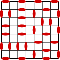
Figure 1: (Color online.) A square lattice with dimer covering. Dimers are indicated by ovals.

The exploration of QDMs has given rise to profound insights into possible realizations of short range RVB spin liquid physics, in particular on non-bipartite lattices.Moessner and Sondhi (2001); Misguich et al. (2002) It has remained challenging, however, to rigorously establish the status of simple QDMs as viable effective theories for quantum spin-$1/2$ systems within a certain parameter regime. The lack of orthogonality of the NNVB states that QDMs seek to describe makes it difficult to establish a direct mapping between QDMs and the low energy sector of quantum spin-$1/2$ models. This difficulty can be dealt with by treating the non-orthogonality as a “small parameter”, and setting up a systematic expansion in this parameter. This notion already played a central role in the original literature,Rokhsar and Kivelson (1988); Sutherland (1988) and was recently explored in great detail in a series of insightful papers.Poilblanc, Mambrini, Schwandt (2010); Schwandt, Mambrini, Poilblanc (2010) Within this scheme, one can thus get the issue of the non-orthogonality of the NNVB states under control. However, the validity of this perturbative scheme depends crucially on the fact that the NNVB states, while not orthogonal, are at least linearly independent, like their counterparts in QDMs. In technical terms, the overlap matrix obtained from the NNVB states must be invertible. The need for an invertible overlap matrix was noticed early on,Rokhsar and Kivelson (1988) and from thereon linear independence of NNVB states was routinely quoted as an assumption in the literature, e.g. in estimates of the low temperature entropy of highly frustrated quantum magnets.Elser (1989); Nussinov et al. (2007) Furthermore, exactly solvable, $SU(2)$-invariant spin-$1/2$ models with RVB and/or spin liquid ground states on simple lattices have only been constructed quite recently,Fujimoto (2005); a_seidel09 (2009); Cano and Fendley (2009); Yao and Lee (2010) in addition to work on decorated lattices.Raman et al. (2005) In Ref. a_seidel09, 2009, rigorous (albeit partial) statements on the uniqueness of the RVB-type ground states of the model constructed there were intimately tied to the linear independence of NNVB states on the kagome lattice. We also note that from a purist point of view, there is a need to demonstrate that superpositions of NNVB wave functions, which may be considered as variationalSutherland (1988); Elser (1989); Nussinov et al. (2007); Flocke et al. (1998); Noorbakhsh et al. (2007) or exactFujimoto (2005); a_seidel09 (2009); Cano and Fendley (2009) solutions to various problems, do not vanish identically, whenever the overlaps between the NNVB states forming these wave functions do not have a uniform sign. The normalizability of such wave functions is an obvious byproduct of the linear independence of NNVB states (on the respective lattice). The explicit or implicit assumption of the linear independence of the NNVB states is thus a prevalent theme in the literature on short range RVB physics, and in some cases has been studied extensively on finite clusters.Mambrini and Mila (2000); Misguich1 et al. (2002)

Rigorous proofs of this linear independence have been available since 1989, through a seminal work of Chayes, Chayes, and Kivelson.Chayes et al. (1989) The proof, however, has been limited to three different types of planar lattices, the square, honeycomb, and square-octagon lattice, and only for the case of open boundary conditions. Here we discuss a more general method, that can, in principle, be applied to any lattice, in the presence of both open and periodic boundary conditions. While we usually have Born–von Karman periodic boundary conditions in mind which give a rectangular (or parallelogram) lattice strip the topology of a torus, our method applies to other lattice topologies as well. To demonstrate this, we also apply our method to the C₆₀ lattice and other fulleren-type lattices, where the linear independence of NNVB (or “Kekulé”) states has direct applications in chemistry.Flocke et al. (1998)

Although there is no guarantee that our proof strategy works for every lattice where the linear independence holds, we demonstrate its applicability to many new two-dimensional (2D) lattices, for which the linear independence of NNVB states is first established in this work. At the same time, we generalize the aforementioned previous results on linear independence of NNVB states to the case of periodic boundary conditions. It is well known that the physics of short range RVB states becomes enriched in subtle ways when periodic boundary conditions are imposed. On a toroidal square lattice, e.g., NNVB states come in a large number of topological sectors characterized by two integer winding numbers $(n_{x},n_{y})$. (For a review, see e.g. Ref. Misguich and Lhuillier, 2005). When the same lattice is viewed as a rectangle with open boundary conditions, the remaining allowed NNVB state all belong to a subset of just the $(0,0)$ sectors. In the thermodynamic limit, the number of NNVB states for open boundary conditions thus becomes a vanishing fraction of the corresponding number for periodic boundary conditions. It is thus clear that the statement of linear independence becomes considerably stronger for periodic boundary conditions, and is often desirable in applications.

We proceed by applying and refining a method that has recently been developed for the kagome lattice,a_seidel09 (2009) making it amenable to more general lattice structures. In Section II.1 we review this method. In Section II.2 we report that this method can be applied without much alteration to the honeycomb lattice, the star lattice, the square-octagon lattice, the squagome lattice, two types of pentagonal lattices (studied in a magnetic context, e.g., in Refs. Moessner and Sondhi, 2001 and Raman et al., 2005), three types of “martini” lattices,Ziff and Scullard (2006) and two types of archimedean lattices. In Section II.3, we apply the same method to fulleren-type lattices. We find that the case of the square lattice requires a generalization of this method, which is introduced and applied in Section II.4. In Section III we summarize our results and discuss possible further applications.

II Method and results

II.1 Derivation of the linear independence condition

In this section we review the method used in Ref. a_seidel09, 2009 to prove the linear independence of the nearest neighbor valence bond states on the kagome lattice. We find that this method can be extended straightforwardly to most other lattices to be considered here. A refinement necessary to study the case of the square lattice will be given further below.

The general starting point of this method is the identification of a suitable (ideally, smallest) cell for which a rather strong local linear independence property holds true. This local linear independence property can conveniently be verified numerically, although in many cases an analytic proof seems feasible as well. As shown in Ref. a_seidel09, 2009, this local property then implies the linear independence of nearest neighbor valence bond states on arbitrarily large lattices that can, in a certain sense, be covered by such cells.not (a) To make this paper self-contained, we will repeat the proof in the following. For the kagome lattice, the smallest possible cell that satisfies these requirements is the 19-site “double star” shown in Fig. (2).

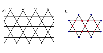
Figure 2: (Color online.) The kagome lattice. a) shows the structure of the kagome lattice, while b) shows the minimal (smallest) cell for which the local independence property defined in the text was proven.a_seidel09 (2009) Different dots are used to label the sites which are defined as inner and outer sites, respectively.

For any given cell of a lattice, we define as interior or inner sites of the cell those sites for which all nearest neighbors are also contained within the cell. Here, the nearest neighbors of a site are all sites connected to it through a link of the lattice. Sites that are not interior are called the boundary sites of the cell. For the kagome cell depicted in Fig. (2), all sites belonging to one of the internal hexagons are interior, while the remaining ones are boundary sites, unless the cell happens to be at a boundary of the lattice itself. In this work we will, however, mostly consider lattices without boundary. Statements about lattices with boundary can then be obtained as simple corollaries. Therefore, the distinction between interior and boundary sites within a cell such as shown in Fig. (2) will not depend on the position of the cell within the lattice.

To proceed, we will now define a certain class of states living on the local cells. We will refer to these states as “local valence bond states”. This does, however, not imply that these states completely dimerize the cell, i.e. that every site of the cell must participate in a valence bond within the cell. Rather, we think of these states as local “snapshots” of a lattice that is in a (globally defined) nearest neighbor valence bond state. In such a snapshot, every internal site of the cell must certainly form a valence bond with one of its nearest neighbors within the cell. A boundary site of the cell, however, may or may not participate in a valence bond with a site within the cell under consideration. In particular, it may participate in a valence bond with a site outside that cell. In the latter case, the local density matrix describing the state of the cell contains no information about the state of the spin of such a boundary site. This motivates the following definition of local valence bond “snapshot” states on the cell $\cal C$. Let us consider states of the form

$$|D\rangle\times|\psi_{f}\rangle\;.$$ (1)

Here, $D$ represents a dimer covering of the cell $\cal C$. By this we mean a pairing of the sites of the cell $\cal C$ into nearest neighbor pairs, where each internal site is a member of a pair, but not necessarily each boundary site. An example for such a pairing is given for the cell of the star lattice shown in Fig. (3d), and that of the square lattice shown in Fig. (10c). By $|D\rangle$ we denote a state where each pair of $D$ forms a singlet, with an arbitrary phase convention. In Eq. (1), the state $|\psi_{f}\rangle$ then denotes any state of the “free” sites that are left untouched by the dimer covering $D$. This can again be seen in Figs. (3d), (10c). In (10c), every dimer covering $D$ leaves behind at least one free site, because of the odd number of sites in this cell. For cells of even size, we leave it understood that the factor $|\psi_{f}\rangle$ in Eq. (1) is absent if $D$ covers all sites of the cell.

We find it convenient to denote by ${\cal H}(D,{\cal C})$ the linear space formed by all local states of the form (1), for a fixed dimer covering $D$, and will also write ${\cal H}(D)$ instead of ${\cal H}(D,{\cal C})$ whenever it is clear what cell is being referred to. The space spanned by all states of this form, without fixing $D$, is called the local valence bond space of the cell ${\cal C}$, $VB({\cal C})$:

$$VB({\cal C})=\sum_{D}{\cal H}(D,{\cal C})\;.$$ (2)

Here, the sum denotes the linear span. For a given cell ${\cal C}$, we will now ask whether the sum in Eq. (2) is direct. This means that the expansion of any state in $VB({\cal C})$ into members of the various spaces ${\cal H}(D)$ is possible in one and only one unique way. Whenever this property holds for some cell ${\cal C}$, we will say that the NNVB states are “locally independent” on the cell ${\cal C}$, or satisfy the “local independence property” on the cell ${\cal C}$.

The local independence property, whenever it can be established for some cell ${\cal C}$, extends to arbitrarily large lattices that can be covered by cells of this topology. Said more precisely, we require that every link of the lattice belongs to a cell that has the topology of ${\cal C}$.not (a) The linear independence of NNVB states defined on the entire lattice can then be seen as follows.a_seidel09 (2009) If the sum in Eq. (2) is direct, then linear projection operators $P_{D}$ acting on the cell ${\cal C}$ are well defined, which project onto the subspaces ${\cal H}(D)$. Said differently, the defining properties of these operators are

$$\begin{split}P_{D}\;{|D^{\prime}\rangle}\otimes{|\psi_{f}\rangle}&=\delta_{D,D^{\prime}}\,{|D^{\prime}\rangle}\otimes{|\psi_{f}\rangle}\,,\\ \text{hence}\;\;P_{D}P_{D^{\prime}}&=\delta_{D,D^{\prime}}P_{D}\;.\end{split}$$ (3)

We note that since the spaces ${\cal H}(D)$ are not orthogonal, the linear projection operators thus defined are not Hermitian. We also mention that to define these operators in within the full $2^{|{\cal C}|}$ dimensional Hilbert space of the cell ${\cal C}$, we need to specify their action on a suitably chosen complement of the local valence bond space $VB({\cal C})$, which can be done in an arbitrary way. In the following, we will only need to know the action of these operators within the subspace $VB({\cal C})$.

The operators $P_{D}$ can now be defined for any cell ${\cal C}$ of some lattice ${\cal L}$, for which the nearest neighbor valence bond states are locally independent in the sense defined above. We may write $P^{\cal C}_{D}$ to explicitly refer to the cell ${\cal C}$ on which these operators act, but will continue to write $P_{D}$ instead whenever no confusion is possible. Armed with these operators, we may consider a general linear relation of the form

$$\sum_{D^{\prime}}\lambda_{D^{\prime}}|D^{\prime}\rangle=0\;.$$ (4)

Here, $D^{\prime}$ now represents a full dimerization of the entire lattice, and for simplicity, we assume that the lattice has no boundary, and can be covered by a single type of cell, as defined above. We will comment on the (simpler) case where the lattice has a boundary below. The states $|D^{\prime}\rangle$ are thus NNVB states of the lattice ${\cal L}$. For definiteness, we may think of, e.g., a honeycomb lattice with periodic boundary conditions. The honeycomb lattice and its smallest cell for which the local independence property holds are shown in Fig. (4). We want to show that Eq. (4) implies that all coefficients $\lambda_{D^{\prime}}$ are zero. For this we first focus on a single cell ${\cal C}$ of the lattice that has the topology shown in Fig. (4b), and a fixed dimer covering $D$ of the entire lattice. The dimer covering $D$ determines a dimer covering $D_{\cal C}$ of the cell ${\cal C}$, consisting of those dimers of $D$ that are fully contained in ${\cal C}$. Consider the action of the operator $P_{D_{\cal C}}$ defined for the cell ${\cal C}$ on any of the states $|D^{\prime}\rangle$ in Eq. (4). Clearly, the dimer covering $D^{\prime}$ determines a local dimer covering of ${\cal C}$, $D^{\prime}_{\cal C}$, defined analogous to $D_{\cal C}$. From the definition of the projection operators, Eq. (3), we see that

$$P_{D_{\cal C}}|D^{\prime}\rangle=\delta_{D_{\cal C},D^{\prime}_{\cal C}}|D^{\prime}\rangle\,.$$ (5)

This is so since the state $|D^{\prime}\rangle$ is contained in the tensor product ${\cal H}(D^{\prime}_{{\cal C}},{\cal C})\otimes{\cal H}({\cal L}\setminus{\cal C})$, where the second factor denotes the Hilbert space associated with all lattice sites not contained in ${\cal C}$. $P_{D_{\cal C}}$ only acts on the first factor, and does so according to Eq. (3). Some further (but trivial) details are explicitly written in Ref. a_seidel09, 2009. Hence, when $P_{D_{\cal C}}$ acts on Eq. (4), one obtains a similar linear combination on the left hand side, but with all dimer coverings $D^{\prime}$ omitted for which the cell ${\cal C}$ does not contain exactly the same dimers as for $D$. We can proceed by successively acting on this new linear relation with the operators $P_{D_{{\cal C}^{\prime}}}$, where $D$ is the same as before, but ${\cal C}^{\prime}$ now runs over all cells of the lattice with the same topology as ${\cal C}$. Since by assumption, these cells cover the lattice in the sense defined above, only those states $|D^{\prime}\rangle$ in Eq. (4) survive this procedure whose underlying dimer covering $D^{\prime}$ looks the same as $D$ everywhere, i.e., only the term with $D^{\prime}=D$ survives. The resulting equation is thus $\lambda_{D}|D\rangle=0$, which implies $\lambda_{D}=0$. Hence $\lambda_{D^{\prime}}=0$ for each dimer covering $D^{\prime}$, since $D$ was arbitrary. This then proves the linear independence of the nearest neighbor valence bond states on the lattice ${\cal L}$.

So far we have considered lattices with periodic boundary conditions. The above result, however, immediately carries over to lattices with a boundary. Let us consider any lattice ${\cal L}^{\prime}$ with an edge that can be obtained from a lattice ${\cal L}$ with periodic boundary conditions, for which the linear independence of NNVB states has been proven, by means of the removal of certain boundary links. Then the set of full dimerizations $D$ of ${\cal L}^{\prime}$ is just a subset of those of ${\cal L}$, and likewise the corresponding set of NNVB states. Hence, if the linear independence of NNVB states holds for ${\cal L}$, it must also hold for ${\cal L}^{\prime}$. More generally, it is easy to see that our result applies to any sublattice ${\cal L}^{\prime}$ of ${\cal L}$, such that ${\cal L}={\cal L}^{\prime}\cup{\cal L}^{\prime\prime}$ is a disjoint union, and both ${\cal L}^{\prime}$ and ${\cal L}^{\prime\prime}$ are fully dimerizable.

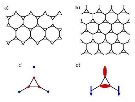
Figure 3: (Color online.) The star lattice (a), and its minimal cell (c) for which the local independence property could be established. (b) shows the martini-A lattice, with the same minimal cell (c). Different shades (colors) of dots identify internal and boundary sites. (d) shows a possible dimer covering: the internal sites must be touched by a dimer, boundary sites may or may not form a dimer (valence bond) with an internal site. In a local valence bond state, boundary sites not participating in valence bonds may be in an arbitrary spin configuration.

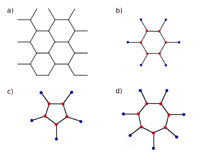
Figure 4: (Color online.) Honeycomb and related structures. (a) The honeycomb lattice. (b) its minimal cell with internal and boundary sites identified. (c) The minimal cell of the buckyball lattice (Fig. (9)). (d) A similar heptagonal cell that also satisfied the local independence property.

II.2 Twelve different 2D lattices

We now discuss the applicability of this method to various two-dimensional lattices. As discussed in Section II.1, this merely requires the identification of a cell of the lattice, for which the local independence property holds, and which can cover the entire lattice in the sense defined there. Such cells have also been dubbed “bricks of linear independence” in Ref. a_seidel09, 2009. For brevity, we will refer to the cells identified by us as “minimal cells”, since there are presumably (in some case obviously) no smaller cells with this property on the respective lattices. We have, however, not carefully ruled out the existence of smaller cells in all cases, since this is of limited interest once sufficiently small “bricks of linear independence” have been identified. For the cell ${\cal C}$ in question, we pick an appropriate basis $|D\rangle\otimes|\psi_{i}\rangle$ for each space ${\cal H}(D)$, where $i=1\dots 2^{n_{D}}$, and $n_{D}$ is the number of sites of the cell ${\cal C}$ that do not participate in the local dimer recovering $D$. The local independence property introduced in the preceding section is then equivalent to the statement that the overlap matrix

$$M_{D^{\prime},j;D,i}=(\langle D^{\prime}|\otimes\langle\psi_{j}|)\,(|D\rangle\otimes|\psi_{i}\rangle)$$ (6)

has full rank. It is clear that for a suitable choice of the factors $|\psi_{i}\rangle$, e.g. “Ising”-type basis states with well-defined local $S_{z}$, and suitable overall normalization factors, the matrix elements $M_{D^{\prime},j;D,i}$ are integer. The question of the rank of this matrix can then be addressed using integer arithmetic free of numerical errors. We did this by using the LinBox package.Lin (2008) By choosing the $\psi_{i}$ from an Ising-$S_{z}$ basis, the matrix in Eq. (6) is also block diagonal with blocks of definite total $S_{z}$. This let to manageable matrix sizes in all the cases discussed in this section.

We present twelve different 2D lattices which we successfully studied using the method described above, and their respective minimal cells ${\cal C}$, for which the local independence has been found to hold, Figs. 2-8. These are, in order, the kagome lattice (treated in Ref. a_seidel09, 2009), the star lattice, the martini-A lattice, the honeycomb lattice, the square-octagon lattice, the squagome lattice, the pentagonal and the “Cairo” pentagonal lattice, 2 more types of the“martini” lattice (martini-B and martini-C), and two types of so called archimedean lattices, denoted archimedean-A and archimedian-B. As proven above, for all these lattices, the identification proper “bricks of linear independence” implies the linear independence NNVB states for arbitrarily large lattices of this type (which must also be large enough to contain the minimal cell), for both open and periodic boundary conditions. For the square-octagon and the honeycomb lattices, the case of open boundary conditions had already been treated in Ref. Chayes et al., 1989 by a different method.

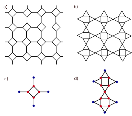
Figure 5: (Color online.) The square-octagon lattice (a) and the squagome lattice (b). (c) and (d) show the respective minimal cells.

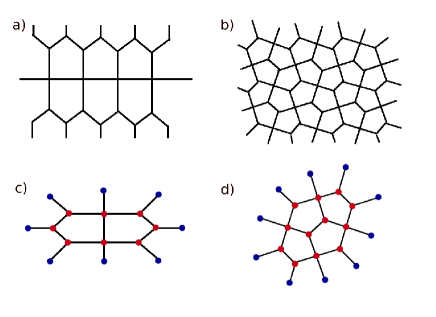
Figure 6: (Color online.) Two types of pentagonal lattices. (a) shows the pentagonal lattice and (b) shows the “Cairo” pentagonal lattice structure, (c) and (d) the respective minimal cells.

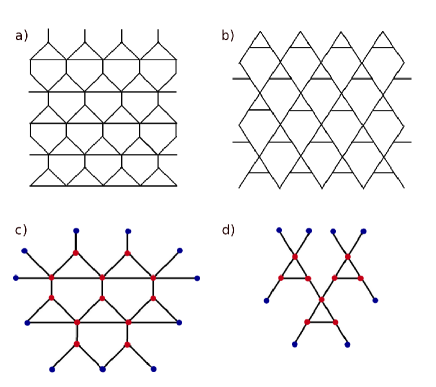
Figure 7: (Color online.) Two more types of martini lattices. (a) and (b) show the lattice structures of the martini-B lattice and the martini-C lattice, respectively, (c) and (d) the respective minimal cells.

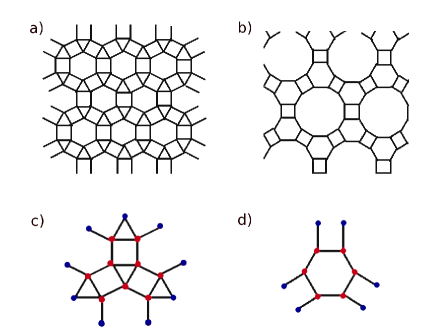
Figure 8: (Color online.) Two types of archimedean lattices. (a) shows the archimedean-A lattice and (b) shows the archimedean-B lattice structures, (c) and (d) the respective minimal cells. Note that the minimal cell in (d) is the same as that of the honeycomb lattice, Fig. (4b).

It is interesting to note that the size of the matrix in Eq. (6) differs quite significantly for the 2D lattices discussed here: for the star and the martini-A lattice, which share the same minimal cell (Fig. (3)), the total matrix dimension (over all $S_{z}$-blocks) is only 13. For others, the matrix dimension is on the order of a few thousand, and for the square lattice cell treated separately in Section II.4, the set of “local valence bond” states $|D\rangle\otimes|\psi_{i}\rangle$ defining the matrix has more than half a million elements.

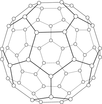
Figure 9: The lattice of the C₆₀ molecule, or “buckyball”. The lattice can be covered by the minimal cell of the honeycomb lattice, Fig. (4b). The actual minimal cell of this lattice is the pentagonal cell shown in Fig. (4c).

II.3 Fullerene-type lattices

We now consider fullerene-type lattices, where each site has three nearest neighbors, and belongs to at least one hexagonal plaquette, where no two members of the same hexagonal plaquette share a nearest neighbor outside that plaquette. Such lattices can be covered, in the sense defined in Section II.1, by the minimal cell of the honeycomb lattice, Fig. (4b). A famous example is the “Buckyball” lattice, Fig. (9). By the results of the preceding sections, the NNVB states on these types of lattices are are linearly independent. This also demonstrates that our method, being essentially local, can be applied to general lattice topologies. not (a)

The Heisenberg model on fulleren-type lattices has been extensively studied within the NNVB subspace in Ref. Flocke et al., 1998 (there called Kekulé subspace). Good agreement with exact diagonalization results within the full Hilbert space was found. The authors also point out the central importance of the linear independence of the NNVB states to their approach. Since the fullerene lattices are finite in size, conventional brute-force numerics may in principle be used to establish this, although the feasibility of this depends, of course, on the actual lattice size. In contrast, the result derived here holds for arbitrarily large systems, and, given the small size of the minimal cells involved, could be obtained purely analytically. In this regard, it is worth noting that the actual minimal cell of the C₆₀ molecule is not that of the honeycomb lattice, Fig. (4b), but the smaller pentagonal cell of Fig. (4c). We have verified that it likewise satisfies the local independence property, and each link of the Buckyball lattice belongs to such a cell. For this rather small cell, an analytic proof of the local independence property seems feasible using the Rumer-Pauling method Rumer (1932); Pauling (1933); Mazumdar and Soos (1979); Ramasesha and Soos (1984) referred to in the next section.

Based on the observations made thus far, we conjecture that all cells where the $n$ inner sites form a single polygon, and each inner site is linked to exactly one of $n$ boundary sites, have the local independence property. Examples of such cells, for which we have verified this, are given in Figs. (3c), (5c), and (4b-d), corresponding to $n=3,4,5,6,7$. For all lattices that can be covered by any combination of such cells (see Ref. not, a), we thus have the linear independence of NNVB states.

II.4 The square lattice

Figure 10: (Color online.) The square lattice. The general lattice structure is shown in Fig. (1). (a) The minimal cell for which the refined local independence property of Section II.4 holds. (b) A local valence bond state with the central site forming a bond with its upper neighbor, corresponding to $\sigma=\uparrow$ as defined in the text.

We find that the method presented in Sec. II.1 cannot immediately be applied to the square lattice. The problem can be traced back to the fact that any local cell on this lattice necessarily that 90 degree corners. It turns out that by using the degrees of freedom near these corners, one can always form non-trivial relations between the states in different subspaces ${\cal H}(D)$. The projection operators in Eq. (3) are then ill-defined. We thus have to modify our method in order to deal with this case. Luckily, the local independence property introduced in Sec. II.1, while it is found to hold for many lattice types, is overly restrictive. In fact, whenever this property holds, it can be literally extended to arbitrarily large lattices with an edge.a_seidel09 (2009) That is, for an arbitrarily large lattice ${\cal L}$, not only states $|D\rangle$ corresponding to full dimerizations of ${\cal L}$ are then linearly independent, but in fact all states of the form $|D\rangle\otimes|\psi_{i}\rangle$, where $D$ does not necessarily cover all boundary sites of ${\cal L}$, and the factors $|\psi_{i}\rangle$ form a basis of the space associated with “free” boundary sites. Clearly, this is a stronger statement than just the linear independence of NNVB states corresponding to full dimerizations of the lattice. However, for the square lattice this stronger property simply does not hold. On the other hand, this “strong” linear independence property is not of primary interest. We are still interested in the linear independence of NNVB states associated with full dimerizations of the lattice, for which the stronger property is not necessary.

It turns out that a weaker version of the local independence property is sufficient to construct suitable projection operators for our purpose. To see this, note that the operators $P_{D}$ defined in Eq. (3) are sensitive to the entire configuration of valence bonds fully contained within the cell on which they act. To prove the linear independence of NNVB states, it is sufficient to work with operators that are sensitive, say, to the bonding state of any given site, as determined by which nearest neighbor this central site is bonding with. To accomplish this, we consider a square lattice ${\cal L}$ satisfying periodic boundary conditions, which is large enough to contain the cell ${\cal C}$ depicted in Fig. (10b). For this cell, we consider four subspaces of $VB({\cal C})$, according to the bonding state of the central site. We define local dimer coverings $D$ of ${\cal C}$ as before, where boundary sites of ${\cal C}$ need not be covered. By $\sigma(D)$ we denote the bonding state of the central site, i.e., $\sigma(D)=\uparrow,\downarrow,\leftarrow,\rightarrow$, depending on whether this site is paired with its upper, lower, left, or right neighbor in the covering D, respectively. As mentioned initially, the sum Eq. (2) defining the space of local valence bond states, $VB({\cal C})$, is not direct for the present cell. However, we may also write the space $VB({\cal C})$ as a “courser” sum of fewer spaces, each of which is formed by all valence bond states that have the central site in a certain bonding state:

$$VB({\cal C})=\sum_{\sigma^{\prime}}VB_{\sigma^{\prime}}({\cal C})\;,$$ (7)

where

$$VB_{\sigma^{\prime}}({\cal C})=\sum_{\begin{subarray}{c}D\\ \sigma(D)=\sigma^{\prime}\end{subarray}}{\cal H}(D,{\cal C})\;,$$ (8)

and $\sigma^{\prime}$ runs over all possible values $\uparrow,\downarrow,\leftarrow,\rightarrow$.

The key observation that renders the square lattice amenable to our method is that the sum in Eq. (7) is still direct. To show this, one must show that the dimensions of the spaces on the right hand side add up to the dimension of the space $VB({\cal C})$. For this it is sufficient to consider the matrix $M$ defined in Eq. (6), together with the matrices $M_{\sigma^{\prime}}$ that are the submatrices of $M$ corresponding to the subspaces $VB_{\sigma^{\prime}}({\cal C})$, and show that the ranks of the $M_{\sigma^{\prime}}$’s add up to that of $M$. Intuitively speaking, this means that while the states $|D\rangle\otimes|\psi_{i}\rangle$, as defined below Eq. (6), satisfy non-trivial linear relations, all these linear relations can be restricted to involve members of the same subspace $VB_{\sigma^{\prime}}({\cal C})$; there are then no further linear relation between members of different subspaces. If the sum in Eq. (7) is indeed direct, we may introduce projection operators $P_{\sigma^{\prime}}$ onto the components on the right hand side. The defining property of these operators is

$$P_{\sigma^{\prime}}\;{|D\rangle}\otimes{|\psi_{i}\rangle}=\delta_{\sigma^{\prime},\sigma(D)}\,{|D\rangle}\otimes{|\psi_{i}\rangle}\,.$$ (9)

When acting on local valence bond states ${|D\rangle}\otimes{|\psi_{i}\rangle}$ living on the cell ${\cal C}$, the operator $P_{\sigma}$ will thus annihilate the state if the bonding state of the central site in the dimer covering $D$ is different from $\sigma$, and otherwise leave the state invariant. It is clear that any site $i$ of the periodic (and sufficiently large) lattice ${\cal L}$ can be made the central site of a cell that has the topology of ${\cal C}$, Fig. (10b). The operators $P_{\sigma}$ defined above can then be extended to the full Hilbert space of the large lattice, and there is an operator $P^{i}_{\sigma}$ for any cell of the type ${\cal C}$ with central site $i$. The defining property (9) then extends to valence bond states $|D\rangle$ corresponding to full dimerizations $D$ of the lattice: $|D\rangle$ survives the action of $P^{i}_{\sigma}$ unchanged if the bonding state of site $i$ in the dimer covering $D$ is $\sigma$, otherwise it is annihilated. Detailed arguments for this are identical to those referred to in Sec. II.1. It is then clear that by successive action with the operators $P^{i}_{\sigma}$, one can single out any dimer covering $D$ in the linear combination Eq. (4), just as carried out in Section II.1, and thus prove that the states $|D\rangle$ are linearly independent.

We have verified that for the cell in Fig. (10b), the sum in Eq. (7) is indeed direct. The numerics were somewhat more challenging, due to size of the 25-site cell under consideration. To wit, this cell admits a total of 5376 different dimer coverings. Each of the dimer coverings has seven “free” outer sites not touched by a dimer, thus the total dimension of the $M$-matrix is a staggering 5376 x 2⁷ = 688128. To reduce the problem to blocks of manageable size, we use the full rotational invariance of the spaces appearing in Eq. (7). That is, we chose the basis $|\psi_{i}\rangle$ for the seven free sites to have a well-defined total spin $S$, in addition to a well-defined $S_{z}$. A suitable choice for a basis is obtained by choosing states corresponding to Rumer-Pauling diagrams.Rumer (1932); Pauling (1933); Mazumdar and Soos (1979); Ramasesha and Soos (1984) The advantage of this is that for appropriate normalization, the matrix elements of the $M$-matrix then remain integer, and we may again make use of exact integer arithmetic.Lin (2008) We further used the mirror symmetry of the cell ${\cal C}$ along one of its diagonals. The largest blocks occurring then had dimensions on the order of 30,000.

The above then establishes that for any sufficiently large square lattice with periodic boundary conditions, the set of all NNVB states is linearly independent. The same statement then follows for lattices with an edge as discussed at the end of Section II.1. The case of general open boundaries conditions has also been treated previously with different methods in Ref. Chayes et al., 1989.

III Summary and discussion

In the preceding sections, we have described a method for proving linear independence of nearest neighbor valence bond states on certain 2D lattices with and without periodic boundary conditions. This method, originally designed for the kagome lattice,a_seidel09 (2009) was successfully extended here to the following lattice types: honeycomb, squagome, pentagonal and Cairo pentagonal, square-octagon, martini-A, -B, and -C, archimedian-A and archimedean-B, and to the star lattice, and furthermore to fullerene-type lattices. Subsequently, a refined method has been developed, which is applicable even in some cases where the original method is inadequate. Specifically, this was found to be the case for the square lattice.

Our method is based on the identification of a certain local independence property for finite clusters, which, when established, implies the linear independence of NNVB states for arbitrarily large lattices. Though here we prefer to validate the local independence property using exact numerical schemes, in those cases where smaller clusters are sufficient, a fully analytic approach is certainly feasible. Further remarks on this for the kagome case, where the cluster size is fairly large, can be found in Ref. a_seidel09, 2009.

We note again that the linear independence of the NNVB states for the square, the honeycomb, and the square-octagon lattice was already established in a paper by Chayes, Chayes, and KivelsonChayes et al. (1989) in 1989. Their result, however, applies only to the case of open boundary conditions. For these lattices, our result extends the one by Chayes et al. to the case of periodic boundary conditions, using a different approach. We have also discussed various applications of these results in RVB inspired approaches to quantum spin-$1/2$ systems.

A case of much interest, which we have not studied here, is that of the triangular lattice. We remark that since the square lattice can be thought of as a triangular lattice endowed with a coarser topology, obtained by removing certain nearest neighbor links, a candidate cell for the triangular lattice would have to be at least as large as our square lattice cell, Fig. (10b), with many more links included. This renders the $M$-matrix so large that we did not find this problem tractable at present. We currently see, however, no fundamental reason why the refined method of the preceding section should not be applicable to this case as well. In all cases thus far studied, we have found that local cells large enough to have more internal sites than boundary sites generally have a sufficiently strong local independence property, which then implies the desired linear independence of globally defined NNVB states. The only exception to this rule seem to be lattices where this “global” linear independence does not hold, for obvious, “local” reasons: These include the checkerboard and the pyrochlore lattice, or any lattice featuring tetrahedral units. By looking at the three dimerizations of a single tetrahedron, it is easy to see that for such lattices, linear independence of NNVB states does not hold. (That is, as long as there is any dimer covering of the lattice with two dimers on the same tetrahedron.)

Thus far, we are not aware of rigorous results on the problem studied here for any three-dimensional lattices (except for finite clusters). We are optimistic, however, that our method is at least applicable to the hyperkagome case, which has recently enjoyed much attention in the study of frustrated quantum magnets.Okamoto et al. (2007); Chen and Balents (2009); Lawler et al. (2008); Zhou et al. (2008); Lawler2 et al. (2008); Bergholtz et al. (2010) A brute force study of the relevant local cell has so far been barred by its size. However, a formal analogy with the kagome case suggests that a partially analytic treatment of the local cell is possible.a_seidel09 (2009) We leave this and other unexplored cases of interest for future studies.