Breakup of the aligned H₂ molecule by xuv laser pulses: A time-dependent treatment in prolate spheroidal coordinates

Abstract

We have carried out calculations of the triple-differential cross section for one-photon double ionization of molecular hydrogen for a central photon energy of $75$ eV, using a fully ab initio, nonperturbative approach to solve the time-dependent Schrödinger equation in prolate spheroidal coordinates. The spatial coordinates $\xi$ and $\eta$ are discretized in a finite-element discrete-variable representation. The wave packet of the laser-driven two-electron system is propagated in time through an effective short iterative Lanczos method to simulate the double ionization of the hydrogen molecule. For both symmetric and asymmetric energy sharing, the present results agree to a satisfactory level with most earlier predictions for the absolute magnitude and the shape of the angular distributions. A notable exception, however, concerns the predictions of the recent time-independent calculations based on the exterior complex scaling method in prolate spheroidal coordinates [Phys. Rev. A 82, 023423 (2010)]. Extensive tests of the numerical implementation were performed, including the effect of truncating the Neumann expansion for the dielectronic interaction on the description of the initial bound state and the predicted cross sections. We observe that the dominant escape mode of the two photoelectrons dramatically depends upon the energy sharing. In the parallel geometry, when the ejected electrons are collected along the direction of the laser polarization axis, back-to-back escape is the dominant channel for strongly asymmetric energy sharing, while it is completely forbidden if the two electrons share the excess energy equally.

I Introduction

A measurement of the complete breakup of the atomic helium target by xuv radiation was achieved over $10$ years ago Brauning1998 . Since then, rapid developments in strong xuv light sources and momentum imaging techniques have made it possible to record all the reaction fragments, nuclei and electrons, in double photoionization of the simplest two-electron hydrogen/deuterium molecule by one-photon absorption Weber-1 ; Weber-2 ; Weber-3 ; Gisselbrecht2006 , and most recently also for two-photon absorption Jiang2010 . For the double ionization of H₂ by single-photon absorption, only randomly oriented molecules were investigated in earlier experiments (e.g. Wightman1998 ). Using “fixed-in-space” molecules, more recent experimental efforts include the measurements of energy- and angle-resolved differential cross sections by Weber et al. for either equal energy sharing Weber-1 ; Weber-2 or asymmetric energy sharing Weber-3 , and by Gisselbrecht et al. Gisselbrecht2006 for equal energy sharing at a photon energy of $76$ eV. These experimental studies were at least partially stimulated by the goal of understanding the similarities and differences between the hydrogen molecule and its atomic counterpart helium. However, all recorded fully differential cross sections to date suffer from some experimental uncertainties regarding the alignment angle of the molecule with respect to the polarization vector of the laser and the emission angles of the photoelectrons.

From a theoretical point of view, the hydrogen molecule exhibits a significant complexity compared to helium and, therefore, provides an enormous challenge to a fully ab initio description inherent in a multi-center, multi-electron system. The single-center convergent close-coupling method was used to model the double ionization of H₂ by Kheifets and Bray Kheifets2005-1 ; Kheifets2005-2 . Later McCurdy, Rescigno, Martín and their collaborators Van2004 ; Van2006-1 ; Van2006-2 implemented a formulation based on time-independent exterior complex scaling (ECS) in spherical coordinates, with the origin of the coordinate system placed at the center of the molecule, to treat the double photoionization at a photon energy of $75$ eV. The radial coordinates of the two electrons are measured from the center, and the radial parts of the wave function were either expanded in $B$-splines or using a finite-element discrete-variable representation (FE-DVR).

The time-dependent close-coupling (TDCC) method Colgan2007 , again in spherical coordinates, was also extended to calculate the triple-differential cross section (TDCS) for double photoionization of the H₂ molecule. While the agreement between the published TDCSs from the ECS Van2006-1 ; Van2006-2 and TDCC Colgan2007 calculations is basically acceptable, noticeable discrepancies remained for a few particular geometries. In the parallel geometry, for instance, where the molecular axis $\bm{\zeta}$ is chosen along the laser polarization vector $\bm{\epsilon}$, the coplanar TDCS predictions from the ECS and TDCC calculations differ by up to $40$ percent when one of the electrons (we will refer to it as the “fixed electron” below) is observed along the direction perpendicular to the $\bm{\epsilon}$-axis. In some other cases, there exists a noticeable “wing” structure in the published TDCC predictions for equal energy sharing. Additional TDCC calculations Colgan2010 suggest that the agreement can be systematically improved, albeit the above-mentioned discrepancy still exists at a somewhat reduced level.

Another independent approach Tao2010 to this problem is the very recent time-independent ECS treatment, formulated – as in the current work – in prolate spheroidal coordinates. Quite surprisingly, the results of that calculation differed from both the earlier ECS and also the TDCC predictions, both obtained in spherical coordinates. Specifically, the ECS prolate spheroidal calculations showed differences from the earlier spherical coordinate calculation for the TDCSs, at a level of about $20\%$ depending on the details of the energy sharing. As will be demonstrated below, we have gone to considerable lengths in an attempt to resolve these discrepancies. However, significant differences between the present results and those of the ECS Tao2010 still remain.

Both the ECS Van2006-1 ; Van2006-2 and the TDCC Colgan2007 calculations made some attempt to deal with the experimental uncertainties in the scattering angles. Given the experimental uncertainties and the differences in the previous calculations, however, it appeared worthwhile to investigate the computational effort required to obtain accurate TDCSs before averaging over any experimental acceptance angles. Consequently, the present calculation represents an independent implementation of the time-dependent FE-DVR approach in prolate spheroidal coordinates. As in the other approaches mentioned above, the internuclear separation ($R$) was held fixed at its equilibrium distance of $1.4$ bohr. The two-center prolate system, with the foci located on the nuclei, provides a suitable description for the two-center characteristics of the H₂ molecule. The formulation of the Schrödinger equation in prolate spheroidal coordinates for diatomic molecules is not new. The pioneering work of Bates, Öpik, and Poots Bates1953 for the H${}_{2}^{+}$ ion, which is exactly separable in prolate spheroidal coordinates, already revealed the appealing features of the prolate system. In particular, the electron-nuclear interaction is rendered benign in this coordinate system. A partial list of recent applications of prolate spheroidal coordinates to diatomic molecules can be found in Bachau2003 ; Barmaki2004 ; Vanne2004 ; Bandrauk2005 ; Tao2009 .

As has been demonstrated in a number of recent publications, a grid-based approach provides a very appropriate description of laser-driven atomic and molecular physics when combined with an efficient time-propagation method such as the short iterative Lanczos (SIL) method Park1986 ; Tannor2007 . In the present work, we employ the FE-DVR/SIL approach in prolate spheroidal coordinates to study the correlated response of a two-electron molecule in the double ionization process.

The remainder of this manuscript is organized as follows. After presenting the Hamiltonian of the hydrogen molecule in Section II and providing some details about the discretization of the system in an FE-DVR basis in Sec. III, the solution of the two-center Poisson equation is presented in Sec. IV. This is followed by a description of the procedure for extracting the cross sections of interest in Sec. V. The results are presented and discussed in Sec. VI, before we finish with a summary in Sec. VII.

II The Schrödinger equation in prolate spheroidal coordinates

The prolate spheroidal coordinates with the two foci separated by a distance $R$ are defined by

$$\xi=\frac{r_{1}+r_{2}}{R},\hskip 8.53581pt\eta=\frac{r_{1}-r_{2}}{R},$$ (1)

and the azimuthal angle $\varphi$. Here $r_{1}$ and $r_{2}$ are the distances measured from the two nuclei, respectively. These coordinates are specified in the ranges $\xi\in[1,+\infty)$, $\eta\in[-1,+1]$, and $\varphi\in[0,2\pi]$. The volume element is $dV=(R/2)^{3}(\xi^{2}-\eta^{2})d\xi d\eta d\varphi$. According to the asymptotic behaviors as $r_{1},r_{2}\rightarrow+\infty$, $\xi$ and $\eta$ approach $2r/R$ and $\cos\theta$, respectively, where $r$ and $\theta$ are the standard spherical coordinates. Consequently, $\xi$ is the “quasi-radial” coordinate, while $\eta$ is “quasi-angular”. The Hamiltonian of a single electron, ${\cal H}_{q}$, ($q=1,2$ for the two electrons in H₂ below), is written as

$${\cal H}_{q}= -\frac{2}{R^{2}(\xi_{q}^{2}-\eta_{q}^{2})}\Bigg{[}\frac{\partial}{\partial\xi_{q}}(\xi_{q}^{2}-1)\frac{\partial}{\partial\xi_{q}}+\frac{\partial}{\partial\eta_{q}}(1-\eta_{q}^{2})\frac{\partial}{\partial\eta_{q}}$$ (2)

$$+ \frac{1}{(\xi_{q}^{2}-1)}\frac{\partial^{2}}{\partial\varphi_{q}^{2}}+\frac{1}{(1-\eta_{q}^{2})}\frac{\partial^{2}}{\partial\varphi_{q}^{2}}\Bigg{]}-\frac{4\xi_{q}}{R(\xi_{q}^{2}-\eta_{q}^{2})}.$$

We solve the time-dependent Schrödinger equation (TDSE) of the laser-driven H₂ molecule (with two electrons) in the dipole length gauge:

$$i\frac{\partial}{\partial t}\Psi(1,2,t)=\Big{[}{\cal H}_{1}+{\cal H}_{2}+\frac{1}{r_{12}}+\bm{E}(t)\cdot(\bm{r}_{1}+\bm{r}_{2})\Big{]}\Psi(1,2,t).$$ (3)

Here ${\bm{r}}_{q}$ is the coordinate of the $q$-th electron measured relative to the center of the molecule and $r_{12}=|\bm{r}_{1}-\bm{r}_{2}|$ is the interelectronic distance. Without loss of generality, we choose the molecular axis along the $z$ axis, and the plane formed by the molecular axis and the polarization vector as the $xz$ plane. Generally, we can decompose the polarization vector into its two components, $\bm{\epsilon}=\cos\theta_{N}\bm{e}_{z}+\sin\theta_{N}\bm{e}_{x}$, where $\theta_{N}$ is the angle between the $\bm{\varsigma}$ and $\bm{\epsilon}$ axes, and $\bm{e}_{z}$ and $\bm{e}_{x}$ are the unit vectors along the $z$ and $x$ axes, respectively. The dipole interaction is therefore given as

$$\bm{E}(t)\cdot(\bm{r}_{1}+\bm{r}_{2})= E(t)\Big{[}(z_{1}+z_{2})\cos\theta_{N}$$

$$+ (x_{1}+x_{2})\sin\theta_{N}\Big{]},$$ (4)

where the rectangular coordinates $x$ and $z$ and the prolate spheroidal coordinates are related through

$$x=\frac{R}{2}\sqrt{(\xi^{2}-1)(1-\eta^{2})}\cos\varphi,\hskip 8.53581ptz=\frac{R}{2}\xi\eta.$$ (5)

We expand the wave function for the H₂ molecule in the body-frame as

$$\Psi(1,2,t)= \sum_{m_{1}m_{2}}\Pi_{m_{1}m_{2}}(\xi_{1},\eta_{1},\xi_{2},\eta_{2},t)$$

$$\times \Phi_{m_{1}m_{2}}(\varphi_{1},\varphi_{2}).$$ (6)

Here $\Phi_{m_{1}m_{2}}(\varphi_{1},\varphi_{2})=e^{i(m_{1}\varphi_{1}+m_{2}\varphi_{2})}/(2\pi)$ is the angular function, where $m_{1}$ and $m_{2}$ denote the magnetic quantum numbers of the two electrons along the molecular axis.

Next, $\Pi_{m_{1}m_{2}}(\xi_{1},\eta_{1},\xi_{2},\eta_{2},t)$ is expanded in a product of normalized “radial” $\{f_{i}(\xi)\}$ and “angular” $\{g_{k}(\eta)\}$ DVR bases:

$$\begin{split}\Pi_{m_{1}m_{2}}(\xi_{1},\eta_{1},\xi_{2},\eta_{2},t)=\\ &\sum_{ijk\ell}f_{i}(\xi_{1})f_{j}(\xi_{2})g_{k}(\eta_{1})g_{\ell}(\eta_{2})C_{ijk\ell}^{m_{1}m_{2}}(t).\end{split}$$ (7)

Note that the basis is not symmetrized with respect to the coordinates of the two electrons. Since we always begin the calculation with a properly symmetrized initial state, however, that symmetry will be preserved in the calculation.

To discretize this partial differential equation, we employ the FE-DVR approach for both the $\xi$ and $\eta$ variables Tao2009 ; Guan2010 . If we normalize the DVR bases according to

$$\int d\xi f_{i}(\xi)f_{i^{\prime}}(\xi)=\delta_{ii^{\prime}}\hskip 5.69054pt\mbox{and}\hskip 2.84526pt\int d\eta g_{k}(\eta)g_{k^{\prime}}(\eta)=\delta_{kk^{\prime}},$$ (8)

respectively, the overall $(\xi,\eta)$ DVR basis is not normalized with respect to the volume element in the prolate coordinate system. This is corrected by defining the two-electron basis

$$b_{ijk\ell}^{m_{1}m_{2}}(1,2)= \Big{(}\frac{2}{R}\Big{)}^{3}\frac{1}{\sqrt{(\xi_{i}^{2}-\eta_{k}^{2})(\xi_{j}^{2}-\eta_{\ell}^{2})}}$$ (9)

$$\times f_{i}(\xi_{1})f_{j}(\xi_{2})g_{k}(\eta_{1})g_{\ell}(\eta_{2})\Phi_{m_{1}m_{2}}(\varphi_{1},\varphi_{2}),$$

which satisfies the desired normalization

$$\iint dV_{1}dV_{2}b_{ijk\ell}^{m_{1}m_{2}*}(1,2)b_{i^{\prime}j^{\prime}k^{\prime}\ell^{\prime}}^{m^{\prime}_{1}m^{\prime}_{2}}(1,2)=$$

$$\delta_{ii^{\prime}}\delta_{jj^{\prime}}\delta_{kk^{\prime}}\delta_{\ell\ell^{\prime}}\delta_{m_{1}m^{\prime}_{1}}\delta_{m_{2}m^{\prime}_{2}},$$ (10)

to expand $\Pi_{m_{1}m_{2}}(\xi_{1},\eta_{1},\xi_{2},\eta_{2},t)$. Specifically, we have

$$\Psi(1,2,t)=\sum_{m_{1}m_{2}}\sum_{ijk\ell}b_{ijk\ell}^{m_{1}m_{2}}(1,2)X_{ijk\ell}^{m_{1}m_{2}}(t).$$ (11)

Introducing the normalized $(\xi,\eta)$ DVR basis eliminates the complexities of matrix operations related to the overlap matrix at each time, and hence makes the standard SIL algorithm directly applicable to study the temporal response of the molecule to laser pulses.

III The FE-DVR basis

In our current implementation of the FE-DVR approach for the time-dependent wave function in prolate spheroidal coordinates, we have chosen to work directly in the FE-DVR basis. This differs from what is usually done for atoms in spherical coordinates, where spherical harmonics are used for the angular variables and an FE-DVR for the radial coordinates. Consequently, the boundary conditions in prolate spheroidal coordinates require some more discussion. Analyzing the asymptotics reveals that in the region near the boundaries of $\xi=1$ and $\eta=\pm 1$, which correspond to the molecular axis, the single-electron wave function behaves like $(\xi^{2}-1)^{|m|/2}(1-\eta^{2})^{|m|/2}$. This indicates that the physical wave function is finite for $|m|=0$, whereas it goes to zero in the region close to the molecular axis for $|m|\neq 0$. More importantly, the behavior of the wave function for odd $|m|$ contains a square-root factor, giving a decidedly nonpolynomial behavior to the wave function that is impossible to capture in a straightforward fashion using a DVR basis.

The former problem is readily treated by using a Gauss-Radau quadrature in the first DVR element for $\xi$, where only the right-most point is constrained to lie on the boundary between the first and second finite element. The volume element ensures that the integrand is well behaved near the end points and makes it unnecessary to invoke a separate quadrature for different $m$ values. For all the other elements, a Gauss-Lobatto quadrature is employed. This allows us to make the FE-DVR basis continuous everywhere and to satisfy the $|m|$-dependent boundary condition.

To overcome the nonanalytic behavior of the basis for odd $m$, Bachau and collaborators Bachau2003 explicitly factored out the $(\xi^{2}-1)^{|m|/2}(1-\eta^{2})^{|m|/2}$ part before the wave function was expanded in terms of $B$-splines in the discretization approach. We have adopted a similar idea in our FE-DVR treatment of the two-center problem to achieve much faster convergence, as was also done in Ref. Tao2009 . For the case of even $|m|$, no changes need to be made to define the DVR basis, i.e., the normalized basis is written as

$$f_{i}(\xi)=\frac{1}{\sqrt{\omega_{\xi}^{i}}}\prod_{k\neq i}\frac{\xi-\xi_{k}}{\xi_{i}-\xi_{k}}\hskip 8.53581pt\text{and}\hskip 8.53581ptg_{i}(\eta)=\frac{1}{\sqrt{\omega_{\eta}^{i}}}\prod_{k\neq i}\frac{\eta-\eta_{k}}{\eta_{i}-\eta_{k}}.$$ (12)

For odd $|m|$, however, we define the DVR basis as

$$f_{i}(\xi)=\frac{1}{\sqrt{\omega_{\xi}^{i}}}\frac{(\xi^{2}-1)^{1/2}}{(\xi^{2}_{i}-1)^{1/2}}\prod_{k\neq i}\frac{\xi-\xi_{k}}{\xi_{i}-\xi_{k}}$$ (13)

and

$$g_{i}(\eta)=\frac{1}{\sqrt{\omega_{\eta}^{i}}}\frac{(1-\eta^{2})^{1/2}}{(1-\eta^{2}_{i})^{1/2}}\prod_{k\neq i}\frac{\eta-\eta_{k}}{\eta_{i}-\eta_{k}}.$$ (14)

Here $\omega_{\xi}^{i}$ and $\omega_{\eta}^{i}$ are the weight factors related to the DVR bases $f_{i}(\xi)$ and $g_{i}(\eta)$, respectively. The goal of using a unique set of mesh points, which are $|m|$-independent, to discretize the $(\xi,\eta)$ coordinates has now been achieved in this scheme. The same technique was employed in recent calculations of one- and two-photon double ionization of H₂ Tao2010 ; Guan2010 . In principle, it is also possible to introduce the factors $(\xi^{2}-1)^{|m|/2}(1-\eta^{2})^{|m|/2}$ into the DVR bases to circumvent the difficulties related to the nonanalytic behavior near the boundary. However, this results in an $|m|$-dependence of the DVR bases and quadrature points. This, in turn, leads to a number of unnecessary complications in the practical implementation of the computational methodology. One might argue that an $|m|$-dependent discretization procedure could be useful for a system in which the magnetic quantum number $m$ is conserved. An example is the H${}_{2}^{+}$ ion in external magnetic fields along the molecular axis Guan2003 . However, that is not the situation in the current calculation.

IV The Electron-Electron Coulomb Interaction in prolate spheroidal coordinates

Similar to the expansion of the electron-electron interaction in terms of spherical coordinates, a counterpart exists in prolate spheroidal coordinates Morse1953 through the Neumann expansion

$$\frac{1}{r_{12}}= \frac{1}{a}\sum_{l=0}^{\infty}\sum_{m=-l}^{l}(-1)^{|m|}(2l+1)\bigg{(}\frac{(l-|m|)!}{(l+|m|)!}\bigg{)}^{2}$$ (15)

$$\times P_{l}^{|m|}(\xi_{<})Q_{l}^{|m|}(\xi_{>})P_{l}^{|m|}(\eta_{1})P_{l}^{|m|}(\eta_{2})e^{im(\varphi_{1}-\varphi_{2})},$$

where $a\equiv R/2$. The two nuclei are located at $\pm R/2$ along the $z$ axis and $\xi_{>(<)}=\max(\min)(\xi_{1},\xi_{2})$. Both the regular $P_{l}^{|m|}(\xi)$ and irregular $Q_{l}^{|m|}(\xi)$ Legendre functions Handbook , which are defined in the region $(1,+\infty)$, are involved in the expansion as the “radial” part, while the “angular” part is only related to $P_{l}^{|m|}(\eta)$. Note that we chose to work in terms of an un-normalized “angular” basis rather than the usual spherical harmonics. The matrix elements of $1/r_{12}$ in a traditional basis, for example, a $B$-spline or Slater-type basis, can be computed through the well-known Mehler-Ruedenberg transformation Vanne2004 ; Mehler1969 . Due to the discontinuous derivative along the line of $\xi_{1}=\xi_{2}$ in the Neumann expansion, the straightforward computation of the matrix element of $1/r_{12}$, using the value of this interaction potential at the mesh points, is very slowly convergent. We seek a more robust representation of the $1/r_{12}$ matrix which retains both the underlying Gauss quadrature and the DVR property of all potentials being exactly diagonal with respect to the highly localized DVR basis.

In the following, we use the simplified notation $|ijk\ell m_{1}m_{2}\rangle=|f_{i}(\xi_{1})f_{j}(\xi_{2})g_{k}(\eta_{1})g_{\ell}(\eta_{2})\Phi_{m_{1}m_{2}}(\varphi_{1},\varphi_{2})\rangle$ to denote the basis. Essentially, we need the integral

$$\Big{\langle}ijk\ell m_{1}m_{2}\Big{|}P_{l}^{|m|}(\xi_{<})Q_{l}^{|m|}(\xi_{>})P_{l}^{|m|}(\eta_{1})P_{l}^{|m|}(\eta_{2})$$ (16)

$$\hskip 45.52458pt\times e^{im(\varphi_{1}-\varphi_{2})}\Big{|}i^{\prime}k^{\prime}j^{\prime}\ell^{\prime}m^{\prime}_{1}m^{\prime}_{2}\Big{\rangle}.$$

After integrating over $\varphi_{1}$ and $\varphi_{2}$, the matrix element of $1/r_{12}$ can be written as

$$\Big{\langle}ijk\ell m_{1}m_{2}|\frac{1}{r_{12}}|i^{\prime}j^{\prime}k^{\prime}\ell^{\prime}m^{\prime}_{1}m^{\prime}_{2}\Big{\rangle}$$ (17)

$$=\frac{1}{a}\sum_{l=|m|}^{\infty}(-1)^{|m|}(2l+1)\bigg{(}\frac{(l-|m|)!}{(l+|m|)!}\bigg{)}^{2}{\cal I}_{ijk\ell}^{i^{\prime}j^{\prime}k^{\prime}\ell}(l),$$

where the selection rule $m=m_{1}-m^{\prime}_{1}=m^{\prime}_{2}-m_{2}$ has been used. Hence $m$ is uniquely determined for a given pair of angular partial waves. Above we introduced the reduced ($\xi,\eta$) integral

$${\cal I}_{ijk\ell}^{i^{\prime}j^{\prime}k^{\prime}\ell^{\prime}}(l)$$ (18)

$$=\big{\langle}ijk\ell\big{|}P_{l}^{|m|}(\xi_{<})Q_{l}^{|m|}(\xi_{>})P_{l}^{|m|}(\eta_{1})P_{l}^{|m|}(\eta_{2})\big{|}i^{\prime}j^{\prime}k^{\prime}\ell^{\prime}\big{\rangle}.$$

Since $|m|$ is fixed in the above equation, we omitted it in ${\cal I}_{ijk\ell}^{i^{\prime}j^{\prime}k^{\prime}\ell^{\prime}}(l)$ and will do so in the related quantities below as well. It is now worthwhile to define the two electron densities McCurdy2004 :

$$\begin{split}\rho_{A}(\xi,\eta)&=f_{i}(\xi)g_{k}(\eta)f_{i^{\prime}}(\xi)g_{k^{\prime}}(\eta),\\ \rho_{B}(\xi,\eta)&=f_{j}(\xi)g_{\ell}(\eta)f_{j^{\prime}}(\xi)g_{\ell^{\prime}}(\eta).\end{split}$$ (19)

After truncating the radial integral to the edge of the box, $\xi_{\rm max}$, this yields

$$\begin{split}{\cal I}_{ijk\ell}^{i^{\prime}j^{\prime}k^{\prime}\ell^{\prime}}(l)&=\iint dV_{\xi}dV_{\xi^{\prime}}\rho_{B}(\xi,\eta)P_{l}^{|m|}(\xi_{<})Q_{l}^{|m|}(\xi_{>})\\ &\times P_{l}^{|m|}(\eta)P_{l}^{|m|}(\eta^{\prime})\rho_{A}(\xi^{\prime},\eta^{\prime})\\ &=\int_{1}^{\xi_{\rm max}}dV_{\xi}P_{l}^{|m|}(\eta)\rho_{B}(\xi,\eta){\cal U}_{l}(\xi).\end{split}$$ (20)

Here a convention for the volume element was made in such a way that, for any function $F(\xi,\eta)$, we define $dV_{\xi}F(\xi,\eta)\equiv d\xi a^{3}\int_{-1}^{+1}(\xi^{2}-\eta^{2})F(\xi,\eta)d\eta$ to simplify the notation. Most importantly, the function ${\cal U}_{l}(\xi)$ is defined by

$${\cal U}_{l}(\xi)= Q_{l}^{|m|}(\xi)\int_{1}^{\xi}dV_{\xi^{\prime}}\rho_{A}(\xi^{\prime},\eta^{\prime})P_{l}^{|m|}(\xi^{\prime})P_{l}^{|m|}(\eta^{\prime})$$ (21)

$$+ P_{l}^{|m|}(\xi)\int_{\xi}^{\xi_{{\rm max}}}dV_{\xi^{\prime}}\rho_{A}(\xi^{\prime},\eta^{\prime})Q_{l}^{|m|}(\xi^{\prime})P_{l}^{|m|}(\eta^{\prime}).$$

Instead of evaluating the above integrals directly, we solve the differential equation satisfied by ${\cal U}_{l}(\xi)$. As will become apparent later, this equation can be shown to be the “radial” Poisson equation in the prolate spheroidal coordinate system. The differential equations satisfied by the Legendre functions $P_{l}^{|m|}(\xi)$ and $Q_{l}^{|m|}(\xi)$ suggests that we introduce the operator

$$\nabla_{\xi}^{2}=\frac{d}{d\xi}(\xi^{2}-1)\frac{d}{d\xi}-l(l+1)-\frac{m^{2}}{\xi^{2}-1}$$ (22)

for given quantum numbers $l$ and $m$. This is the one-dimensional Laplacian operator in the $\xi$ coordinate.

After some algebra, we obtain

$$\frac{d}{d\xi}{\cal U}_{l}(\xi)= \frac{dQ_{l}^{|m|}(\xi)}{d\xi}\int_{1}^{\xi}dV_{t}\rho_{A}(t,\tau)P_{l}^{|m|}(t)P_{l}^{|m|}(\tau)$$ (23)

$$+ \frac{dP_{l}^{|m|}(\xi)}{d\xi}\int_{\xi}^{\xi_{\rm max}}dV_{t}\rho_{A}(t,\tau)Q_{l}^{|m|}(t)P_{l}^{|m|}(\tau).$$

and

$$\begin{split}\frac{d^{2}}{d\xi^{2}}{\cal U}_{l}(\xi)=&\frac{d^{2}Q_{l}^{|m|}(\xi)}{d\xi^{2}}\int_{1}^{\xi}dV_{t}\rho_{A}(t,\tau)P_{l}^{|m|}(t)P_{l}^{|m|}(\tau)\\ +&\frac{d^{2}P_{l}^{|m|}(\xi)}{d\xi^{2}}\int_{1}^{\xi}dV_{t}\rho_{A}(t,\tau)Q_{l}^{|m|}(t)P_{l}^{|m|}(\tau)+\\ +W(P_{l}^{|m|}&(\xi),Q_{l}^{|m|}(\xi))a^{3}\int_{-1}^{+1}\!\!d\tau(\xi^{2}\!-\!\eta^{2})\rho_{A}(\xi,\tau)P_{l}^{|m|}(\tau).\end{split}$$ (24)

Here the Wronskian of the Legendre functions $P_{l}^{|m|}(\xi)$ and $Q_{l}^{|m|}(\xi)$ is given by

$$W(P_{l}^{|m|}(\xi),Q_{l}^{|m|}(\xi))=\frac{(-1)^{|m|}}{(1-\xi^{2})}\frac{(l+|m|)!}{(l-|m|)!}.$$ (25)

Consequently, we obtain

$$\nabla_{\xi}^{2}{\cal U}_{l}(\xi)=\varrho(\xi).$$ (26)

This is the second-order inhomogeneous Poisson equation satisfied by ${\cal U}_{l}(\xi)$ with the “source” term given by

$$\varrho(\xi)= (-1)^{|m|+1}\frac{(l+|m|)!}{(l-|m|)!}a^{3}$$ (27)

$$\times \int_{-1}^{+1}d\eta^{\prime}(\xi^{2}-\eta^{\prime 2})\rho_{A}(\xi,\eta^{\prime})P_{l}^{|m|}(\eta^{\prime}).$$

After carrying out the integral over $\eta^{\prime}$ via Gauss quadrature, we recast the source term as

$$\begin{split}\varrho(\xi)=&\delta_{kk^{\prime}}(-1)^{|m|+1}\frac{(l+|m|)!}{(l-|m|)!}a^{3}f_{i}(\xi)f_{i^{\prime}}(\xi)\\ \times&(\xi^{2}-\eta_{k}^{2})P_{l}^{|m|}(\eta_{k}).\end{split}$$ (28)

As one might expect, the inhomogeneous equation reduces to the homogeneous one if $k\neq k^{\prime}$. The solution to the Poisson equations (26) and (28) can be uniquely determined by enforcing the boundary conditions

$${\cal U}_{l}(1)=P_{l}^{|m|}(1)\int_{1}^{\xi_{\rm max}}dV_{\xi^{\prime}}\rho_{A}(\xi^{\prime},\eta^{\prime})Q_{l}^{|m|}(\xi^{\prime})P_{l}^{|m|}(\eta^{\prime})$$ (29)

at $\xi=1$ and

$${\cal U}_{l}(\xi_{\rm max})=Q_{l}^{|m|}(\xi_{\rm max})\int_{1}^{\xi_{\rm max}}dV_{\xi^{\prime}}\rho_{A}(\xi^{\prime},\eta)P_{l}^{|m|}(\xi^{\prime})P_{l}^{|m|}(\eta^{\prime})$$ (30)

at $\xi=\xi_{\rm max}$, respectively.

There are two important points to realize, namely: First, on the right-hand boundary, the function ${\cal U}_{l}(\xi)$ assumes a nonzero value, which is given by Eq. (30), for all possible $|m|$ values. Its asymptotic behavior relies on the function $Q_{l}^{|m|}(\xi)$ at large $\xi$, which behaves like $1/\xi_{\rm max}^{l+1}$. This indicates that it is nonzero generally, although it could be small at the large $\xi_{\rm max}$ values used in practical calculations. Second, on the left-hand boundary, the situation depends on the value of $|m|$. ${\cal U}_{l}(\xi)$ takes a nonzero value if $|m|=0$, while it becomes zero if $|m|\neq 0$.

Following the philosophy employed to handle the spherical case McCurdy2004 , we first seek a solution, ${\cal U}_{l}^{0}(\xi)$, to the Poisson equations (26)-(30) that satisfies the zero-value boundary condition at $\xi_{\rm max}$ by using exactly the same $\xi$ mesh points as those for the wave functions. In other words, we have $\nabla^{2}_{\xi}{\cal U}_{l}^{0}(\xi)=\varrho(\xi)$ with ${\cal U}_{l}^{0}(1)={\cal U}_{l}(1)$ and ${\cal U}_{l}^{0}(\xi_{\rm max})=0$. After substituting the DVR expansion ${\cal U}_{l}^{(0)}(\xi)=\sum_{\mu}c_{\mu}f_{\mu}(\xi)$ of the solution into the differential equation, we obtain a system of linear equations for the unknown coefficients $\{c_{\mu}\}$:

$$\begin{split}\sum_{\mu^{\prime}}c_{\mu^{\prime}}T_{\mu\mu^{\prime}}^{|m|}=&(-1)^{|m|}\frac{(l+|m|)!}{(l-|m|)!}\frac{1}{\sqrt{\omega_{\xi}^{i}}}a^{3}\delta_{\mu i}\delta_{ii^{\prime}}\delta_{kk^{\prime}}\\ \times&(\xi^{2}_{i}-\eta_{k}^{2})P_{l}^{|m|}(\eta_{k}).\end{split}$$ (31)

The matrix $T$ is defined by its elements

$$T_{\mu\mu^{\prime}}^{|m|}=- \int_{1}^{\xi_{\rm max}}d\xi f_{\mu}(\xi)\bigg{[}(\xi^{2}-1)\frac{d^{2}}{d\xi^{2}}+2\xi\frac{d}{d\xi}$$ (32)

$$- l(l+1)-\frac{m^{2}}{\xi^{2}-1}\bigg{]}f_{\mu^{\prime}}(\xi).$$

Therefore, the coefficient $c_{\mu}$ can formally be written as

$$c_{\mu}=\frac{[T^{|m|}]^{-1}_{\mu i}}{\sqrt{\omega_{\xi}^{i}}}(-1)^{|m|}\frac{(l\!+\!|m|)!}{(l\!-\!|m|)!}a^{3}\delta_{ii^{\prime}}\delta_{kk^{\prime}}(\xi_{i}^{2}-\eta_{k}^{2})P_{l}^{|m|}(\eta_{k}),$$ (33)

where $[T^{|m|}]^{-1}$ denotes the inverse of the matrix $T^{|m|}$. In this case ${\cal U}_{l}^{0}(\xi)$ fulfills the left-hand boundary condition ${\cal U}_{l}^{0}(1)=0$, and so does ${\cal U}_{l}(1)$. Recall, however, that its right-hand boundary condition differs from those of ${\cal U}_{l}(\xi_{\rm max})$. This suggests that the final answer to the function ${\cal U}_{l}(\xi)$ can be constructed as ${\cal U}_{l}(\xi)={\cal U}_{l}^{0}(\xi)+F_{l}(\xi)$, i.e., we add the difference function $F_{l}(\xi)$ to ${\cal U}_{l}^{0}(\xi)$. The function $F_{l}(\xi)$ is also a solution to the homogeneous Poisson equation, subject to the boundary condition $F_{l}(1)=0$ and $F_{l}(\xi_{\rm max})={\cal U}_{l}(\xi_{\rm max})$. After writing it as a linear combination of $P_{l}^{|m|}(\xi)$ and $Q_{l}^{|m|}(\xi)$, and imposing the boundary conditions, $F_{l}(\xi)$ takes the form

$$\begin{split}F_{l}(\xi)=&\delta_{ii^{\prime}}\delta_{kk^{\prime}}a^{3}(\xi_{i}^{2}-\eta_{k}^{2})P_{l}^{|m|}(\xi_{i})P_{l}^{|m|}(\eta_{k})\\ \times&\frac{Q_{l}^{|m|}(\xi_{\rm max})}{P_{l}^{|m|}(\xi_{\rm max})}P_{l}^{|m|}(\xi).\end{split}$$ (34)

We finally arrive at

$$\begin{split}{\cal U}_{l}(\xi)=&\frac{(-1)^{|m|}}{\sqrt{\omega_{\xi}^{i}}}\frac{(l+|m|)!}{(l-|m|)!}a^{3}\delta_{ii^{\prime}}\delta_{kk^{\prime}}(\xi_{i}^{2}-\eta_{k}^{2})P_{l}^{|m|}(\eta_{k})\\ \times&\sum_{\mu}[T^{|m|}]^{-1}_{\mu i}f_{\mu}(\xi)+\delta_{ii^{\prime}}\delta_{kk^{\prime}}(\xi_{i}^{2}-\eta_{k}^{2})P_{l}^{|m|}(\xi_{i})\\ \times&P_{l}^{|m|}(\eta_{k})\frac{Q_{l}^{|m|}(\xi_{\rm max})}{P_{l}^{|m|}(\xi_{\rm max})}P_{l}^{|m|}(\xi).\end{split}$$ (35)

At this point, the DVR version of the solution ${\cal U}_{l}(\xi)$ is ready for all possible values of $|m|$, either $|m|\neq 0$ or $|m|=0$. Substituting Eq. (35) into Eq. (20) allows us to obtain the kernel integral,

$$\begin{split}{\cal I}_{ijk\ell}^{i^{\prime}j^{\prime}k^{\prime}\ell^{\prime}}(l)&=\delta_{ii^{\prime}}\delta_{jj^{\prime}}\delta_{kk^{\prime}}\delta_{\ell\ell^{\prime}}a^{6}(\xi_{i}^{2}-\eta_{k}^{2})(\xi_{j}^{2}-\eta_{\ell}^{2})P_{l}^{|m|}(\eta_{\ell})\\ \times&\Bigg{[}\frac{(-1)^{|m|}}{\sqrt{\omega_{\xi}^{i}\omega_{\xi}^{j}}}\frac{(l+|m|)!}{(l-|m|)!}[T^{|m|}]^{-1}_{ji}P_{l}^{|m|}(\eta_{k})+\\ +&P_{l}^{|m|}(\xi_{i})P_{l}^{|m|}(\xi_{j})P_{l}^{|m|}(\eta_{k})\frac{Q_{l}^{|m|}(\xi_{\rm max})}{P_{l}^{|m|}(\xi_{\rm max})}\Bigg{]}.\end{split}$$ (36)

The matrix element of $1/r_{12}$ can finally be written as

$$\begin{split}\big{<}ijk\ell m_{1}m_{2}\big{|}\frac{1}{r_{12}}\big{|}i^{\prime}j^{\prime}k^{\prime}\ell^{\prime}m^{\prime}_{1}m^{\prime}_{2}\big{>}=&\delta_{ii^{\prime}}\delta_{jj^{\prime}}\delta_{kk^{\prime}}\delta_{\ell\ell^{\prime}}a^{5}(\xi_{i}^{2}-\eta_{k}^{2})(\xi_{j}^{2}-\eta_{\ell}^{2})\sum_{l\geqslant|m|}^{l_{\rm max}}(2l+1)\frac{(l-|m|)!}{(l+|m|)!}P_{l}^{|m|}(\eta_{k})P_{l}^{|m|}(\eta_{\ell})\\ \times&\Bigg{[}\frac{1}{\sqrt{\omega_{\xi}^{i}\omega_{\xi}^{j}}}[T^{|m|}]^{-1}_{ji}+(-1)^{|m|}\frac{(l-|m|)!}{(l+|m|)!}P_{l}^{|m|}(\xi_{i})P_{l}^{|m|}(\xi_{j})\frac{Q_{l}^{|m|}(\xi_{\rm max})}{P_{l}^{|m|}(\xi_{\rm max})}\Bigg{]},\end{split}$$ (37)

where we truncated the $l$ summation in the Neumann expansion to $l_{\rm max}$. The above equation can be converted to the normalized $(\xi,\eta)$ bases with the help of Eq. (9). This results in a diagonal representation of the matrix elements of the electron-electron Coulomb interaction and thus considerably simplifies the FE-DVR discretization procedure. The above treatment of the $1/r_{12}$ matrix was successfully applied to the two-photon double ionization of H₂ Guan2010 . The implementation of this representation will be illustrated below.

V Time Evolution and Extraction of Cross Sections

The time-dependent laser-driven electronic wave packet in the hydrogen molecule is obtained by solving the TDSE on the $(\xi,\eta)$ grid. Launched from the previously determined ground state, the time evolution of the system is achieved by using our recently developed SIL method Guan2008 ; Guan2009 . The ground state is determined by relaxing the system in imaginary time from an initial guess of the wave function on the grid points. At each time step we only need to generate the values of the discretized wave function on the selected grid points. If desired, the information at arbitrary points within the spatial box can be obtained from the interpolation procedure in terms of the DVR bases.

A few remarks seem appropriate regarding the efficient implementation of the SIL algorithm. The highest energy, $E_{\rm max}$, which essentially depends on the smallest separation between the $(\xi,\eta)$ mesh points and also on the maximum values of $|m_{1}|$ and $|m_{2}|$, determines the largest time step $\Delta t$ for the propagation in real time. Typically, $E_{\rm max}$ is about $6,000$ atomic units (a.u.) in our calculations. Although the chances of electrons populating states with such high energies are practically negligible for short time scales of the laser-molecule interaction, we generally require $\Delta t\lesssim 2\pi/E_{\rm max}$ in order to resolve the most rapid oscillations in the time evolution. This means that at least a few time steps are needed during one period of $2\pi/E_{\rm max}$. We refer readers to Refs. Guan2008 ; Guan2009 ; Taylor2003 for further details and discussions behind the SIL method.

In order to ensure that the double-ionization wave packet is sufficiently far away from the nuclei, and also that the two photoelectrons are well separated, we allow the system to evolve for a few more cycles in the field-free Hamiltonian, i.e., after the laser pulse has died off. This is the wave packet we use to extract the physical information. The ionization probabilities and the corresponding cross sections are extracted by projecting the time-dependent wave packet onto uncorrelated two-electron continuum states satisfying the standard incoming boundary conditions. The latter states of H₂ are constructed from the one-electron continuum state of the H${}_{2}^{+}$ ion described in the following subsection.

V.1 Continuum states of H${}_{2}^{+}$

The field-free wave function $\Phi(\xi,\eta,\varphi)$ of the one-electron molecular ion is completely separable in prolate spheroidal coordinates. For a given, and conserved, magnetic quantum number $m$, the wave function takes the form $\Phi(\xi,\eta,\varphi)=T_{m}(\xi)\Xi_{m}(\eta)\Phi_{m}(\varphi)$, where the azimuthal dependence, is given by $\Phi_{m}(\varphi)\equiv e^{im\varphi}/\sqrt{2\pi}$. The “radial” part $T_{mq}(\xi)$ and the “angular” part $\Xi_{mq}(\eta)$ of the wave function satisfy the equations

$$\bigg{[}\frac{\partial}{\partial\xi}(\xi^{2}\!-\!1)\frac{\partial}{\partial\xi}-\frac{m^{2}}{(\xi^{2}\!-\!1)}+2R\xi+c^{2}\xi^{2}-A_{mq}\bigg{]}T_{mq}(\xi)=0$$ (38)

and

$$\bigg{[}\frac{\partial}{\partial\eta}(1-\eta^{2})\frac{\partial}{\partial\eta}-\frac{m^{2}}{(1-\eta^{2})}-c^{2}\eta^{2}+A_{mq}\bigg{]}\Xi_{mq}(\eta)=0,$$ (39)

respectively. Here $c=kR/2$ for the continuum state whose momentum vector has the magnitude $k$. In addition, we need to introduce another quantum number $q$, which denotes the number of nodes of $\Xi_{m}(\eta)$ in the region $\eta\in[-1,+1]$, to label the states, and finally the separation constant $A_{mq}$.

When the angular function $\Xi_{m}(\eta)\Phi_{m}(\varphi)$ is discretized in terms of the relevant DVR bases, a few “spurious” solutions might be encountered. This is caused by the residual errors associated with the Gauss quadratures. Consequently, we expand the angular function, or “spheroidal harmonics” function ${\cal Y}_{\ell m}(\eta,\varphi)\equiv\Xi_{mq}(\eta)\Phi_{mq}(\varphi)$ with $\ell=|m|+q$ instead in terms of spherical harmonics. These functions are normalized according to

$$\int_{-1}^{+1}d\eta\int_{0}^{2\pi}d\varphi{\cal Y}_{\ell m}^{*}(\eta,\varphi){\cal Y}_{\ell^{\prime}m^{\prime}}(\eta,\varphi)=\delta_{mm^{\prime}}\delta_{\ell\ell^{\prime}}.$$ (40)

After obtaining the separation constant $A_{mq}$ by solving Eq. (39), the “radial” function $T_{mq}(\xi)$ is again expanded in terms of the DVR bases. The last DVR point at $\xi=\xi_{\rm max}$ needs to be kept for the continuum state. Asymptotically, the radial function behaves like

$$T_{mq}(\xi)\rightarrow\frac{1}{\xi R}\sqrt{\frac{8}{\pi}}\sin\bigg{[}c\xi+\frac{R}{c}\ln(2c\xi)-\frac{\ell\pi}{2}+\Delta_{mq}(k)\bigg{]}$$ (41)

as $\xi\rightarrow+\infty$. Here $\Delta_{mq}(k)$ is the two-center Coulomb phase shift. The normalization factor on either the energy or the momentum scale and the Coulomb phase shift can be determined by matching the numerical solution of $T_{mq}(\xi)$ according to its asymptotic behavior given in Eq. (41).

The plane wave in prolate spheroidal coordinates can be written as Flammer

$$e^{i\bm{k}\cdot\bm{r}}=4\pi\sum_{\ell m}i^{\ell}{\cal Y}_{\ell m}(\eta_{r},\varphi_{r}){\cal Y}_{\ell m}^{*}(\eta_{k},\varphi_{k})R_{\ell m}^{(k)}(\xi),$$ (42)

where $R_{\ell m}^{(k)}(\xi)\rightarrow 1/(c\xi)\sin\big{[}c\xi-\ell\pi/2\big{]}$ in the asymptotic region. Note that $\eta_{k}$ and $\eta_{r}$ are related to the directions of $\bm{k}$ and $\bm{r}$ in spherical coordinates through $\eta_{k,r}=\cos\theta_{k,r}$. The partial-wave expansion of the plane wave $e^{i\bm{k}\cdot\bm{r}}$ reminds us that the two-center Coulomb wave satisfying the incoming boundary condition can be expanded as

$$\Phi_{\bm{k}}^{(-)}(\bm{r})= \frac{1}{k}\sum_{m=-\infty}^{+\infty}\sum_{\ell\geqslant|m|}i^{\ell}e^{-i\Delta_{mq}(k)}$$

$$\times{\cal Y}_{\ell m}^{*}(\bm{k}){\cal Y}_{\ell m}(\eta_{r},\varphi_{r})T_{mq}^{(k)}(\xi).$$ (43)

This function is normalized in momentum space according to $\langle\Phi_{\bm{k}}^{(-)}|\Phi_{\bm{k}^{\prime}}^{(-)}\rangle=\delta(\bm{k}-\bm{k}^{\prime})$, provided the asymptotic solution in Eq. (41) is satisfied.

Uncorrelated two-electron continuum states with total spin angular momentum $S$ ($S=0$ in our case) can generally be constructed as follows:

$$\Phi_{\bm{k}_{1}\bm{k}_{2}}^{(-)}(\bm{r}_{1},\bm{r}_{2})=$$ (44)

$$\frac{1}{\sqrt{2}}\Big{[}\Phi_{\bm{k}_{1}}^{(-)}(\bm{r}_{1})\Phi_{\bm{k}_{2}}^{(-)}(\bm{r}_{2})+(-1)^{S}\Phi_{\bm{k}_{2}}^{(-)}(\bm{r}_{1})\Phi_{\bm{k}_{1}}^{(-)}(\bm{r}_{2})\Big{]}.$$

With the help of Eq. (43), its partial-wave representation can be written as

$$\Phi_{\bm{k}_{1}\bm{k}_{2}}^{(-)}(\bm{r}_{1},\bm{r}_{2})=\Big{(}\frac{2}{R}\Big{)}^{3}\frac{1}{\sqrt{2}}\frac{1}{k_{1}k_{2}}\sum_{\ell_{1}m_{1}\ell_{2}m_{2}}i^{\ell_{1}+\ell_{2}}$$

$$\hskip 17.07164pt\times\sum_{ijk\ell}b_{ijk\ell}^{m_{1}m_{2}}(1,2)\sqrt{(\xi_{i}^{2}-\eta_{k}^{2})(\xi_{j}^{2}-\eta_{\ell}^{2})}$$ (45)

$$\hskip 17.07164pt\times\Bigg{[}e^{-i\big{(}\Delta_{|m_{1}|\ell_{1}}(k_{1})+\Delta_{|m|_{2}\ell_{2}}(k_{2})\big{)}}{\cal Y}_{\ell_{1}m_{1}}^{*}(\bm{k}_{1}){\cal Y}_{\ell_{2}m_{2}}^{*}(\bm{k}_{2})$$

$$\hskip 36.98857ptC_{ijk\ell}^{\ell_{1}m_{1}\ell_{2}m_{2}}(k_{1},k_{2})+(-1)^{S}(\bm{k}_{1}\leftrightarrow\bm{k}_{2})\Bigg{]}.$$

Here we introduced

$$C_{ijk\ell}^{\ell_{1}m_{1}\ell_{2}m_{2}}(k_{1},k_{2})=$$ (46)

$${\tilde{T}}_{\ell_{1}|m_{1}|}^{(k_{1})}(\xi_{i}){\tilde{T}}_{\ell_{2}|m_{2}|}^{(k_{2})}(\xi_{j}){\tilde{\Xi}}_{\ell_{1}|m_{1}|}^{(k_{1})}(\eta_{k}){\tilde{\Xi}}_{\ell_{2}|m_{2}|}^{(k_{2})}(\eta_{\ell}),$$

by representing the radial and angular parts on the $(\xi,\eta)$ grid points:

$$T_{\ell m}^{(k)}(\xi)=\sum_{i}f_{i}(\xi){\tilde{T}}_{\ell m}^{(k)}(\xi_{i}),$$ (47)

$$\Xi_{\ell m}^{(k)}(\eta)=\sum_{\mu}g_{\mu}(\eta){\tilde{\Xi}}_{\ell m}^{(k)}(\eta_{\mu}).$$ (48)

Here the exchange symmetry

$$C_{ji\ell k}^{\ell_{2}m_{2}\ell_{1}m_{1}}(k_{2},k_{1})=C_{ijk\ell}^{\ell_{1}m_{1}\ell_{2}m_{2}}(k_{1},k_{2})$$ (49)

is satisfied.

V.2 Extraction of double-ionization cross sections

It has been demonstrated Colgan2001 ; Guan2008 ; Guan2010 that using uncorrelated two-electron continuum states is a good approximation in a time-dependent propagation approach, provided the two ejected electrons are well separated from each other. The probability amplitude of double ionization is then given by

$$\langle\Phi_{\bm{k}_{1}\bm{k}_{2}}^{(-)}|\Psi(t)\rangle=$$ (50)

$$\frac{1}{k_{1}k_{2}}\sum_{m_{1}\ell_{1}m_{2}\ell_{2}}(-i)^{\ell_{1}+\ell_{2}}e^{i\big{(}\Delta_{|m_{1}|\ell_{1}}(k_{1})+\Delta_{|m|_{2}\ell_{2}}(k_{2})\big{)}}$$

$$\times{\cal Y}_{\ell_{1}m_{1}}(\bm{k}_{1}){\cal Y}_{\ell_{1}m_{2}}(\bm{k}_{2})\mathfrak{F}_{\ell_{1}m_{1}\ell_{2}m_{2}}(k_{1},k_{2}),$$

where

$$\mathfrak{F}_{\ell_{1}m_{1}\ell_{2}m_{2}}(k_{1},k_{2})=$$ (51)

$$\sqrt{2}\sum_{ijk\ell}C_{ijk\ell}^{\ell_{1}m_{1}\ell_{2}m_{2}*}(k_{1},k_{2}){X}_{ijk\ell}^{m_{1}m_{2}}(t).$$

Here the exchange symmetry

$$\mathfrak{F}_{\ell_{2}m_{2}\ell_{1}m_{1}}(k_{2},k_{1})=(-1)^{S}\mathfrak{F}_{\ell_{1}m_{1}\ell_{2}m_{2}}(k_{1},k_{2})$$ (52)

is satisfied. We also see that the probability amplitude formulated in prolate spheroidal coordinates takes a similar form as for the atomic case in spherical coordinates. However, a subtle difference from the atomic case is worth pointing out. Strictly speaking, the spheroidal harmonics involved in the probability amplitude generally depend on the magnitude of the momenta $k_{1}$ and $k_{2}$, in addition to their directions.

The energy sharing of the two photoelectrons can be specified by introducing the hyperangle $\alpha=\tan^{-1}(k_{2}/k_{1})$. This describes the double-ionization reaction with kinetic energies $E_{1}=E_{\rm exc}\cos^{2}\alpha$ and $E_{2}=E_{\rm exc}\sin^{2}\alpha$ for the two ionized electrons, respectively. Here $E_{\rm exc}$ is the available excess energy above the double-ionization threshold. In the present work, specifically, $E_{\rm exc}=23.6$ eV for absorption of a $75$-eV photon.

For double ionization by one-photon absorption, the triple differential cross section with respect to one of the kinetic energies and the two solid angles $\hat{\bm{k}}_{1}$ and $\hat{\bm{k}}_{2}$ can be extracted using the same formalism as in the corresponding He case Colgan2001 ; Guan2008 , i.e.,

$$\frac{\mbox{d}^{3}\sigma}{\mbox{d}E_{1}\mbox{d}\hat{\bm{k}}_{1}\mbox{d}\hat{\bm{k}}_{2}}=\frac{1}{k_{1}k_{2}\cos^{2}\alpha}\frac{\omega}{I_{0}}\frac{1}{T_{\rm eff}^{(1)}}\int_{0}^{k_{\rm max}}\mbox{d}k^{\prime}_{1}\int_{0}^{k^{\prime}_{1}}\mbox{d}k^{\prime}_{2}$$

$$\times k^{\prime}_{1}\delta(k_{2}^{\prime}-k_{1}^{\prime}\tan\alpha)\Bigg{|}\sum_{m_{1}\ell_{1}m_{2}\ell_{2}}(-i)^{\ell_{1}+\ell_{2}}e^{i\big{(}\Delta_{|m_{1}|\ell_{1}}+\Delta_{|m|_{2}\ell_{2}}\big{)}}$$

$$\times{\cal Y}_{\ell_{1}m_{1}}(k^{\prime}_{1},\hat{\bm{k}}_{1}){\cal Y}_{\ell_{2}m_{2}}(k^{\prime}_{2},\hat{\bm{k}}_{2})\mathfrak{F}_{\ell_{1}m_{1}\ell_{2}m_{2}}(k^{\prime}_{1},k^{\prime}_{2})\Bigg{|}^{2}.$$ (53)

Here $\omega$ and $I_{0}$ are the central photon energy and the peak intensity of the laser pulse, respectively, while $T_{\rm{eff}}^{(1)}$ denotes the effective interaction time between the temporal electric laser field and the electrons in the one-photon absorption process. For a laser pulse of time duration $\tau$ with a sine-squared envelope for the field amplitude, $T_{\rm{eff}}^{(1)}=(3/8)\tau$. Note that $T_{\rm eff}^{(1)}$ corresponds to the special case of the generalized $N$-photon effective interaction time $T_{\rm eff}^{(N)}$ Nikolo2006 for a one-photon reaction. Generalized cross sections for two-photon double ionization of the hydrogen molecule were extracted in the same formalism Guan2010 .

In the TDCC treatment Colgan2007 , different strategies were employed to describe the linear one-photon and the nonlinear two-photon double ionization processes of atoms and molecules. For the one-photon case, the cross sections were obtained through the time derivative of the double-ionization probability, $\partial P_{\rm ion}^{2+}(t)/\partial t$. The laser field does not need to be turned off in this case. On the other hand, a true laser pulse was used for the two-photon case and an effective time, defined as the time integral under a flat-top pulse with a smooth turn-on and turn-off, was introduced. In the present work, we employed a unified formulation through an effective interaction time for both one-photon and multi-photon ionization in laser pulses.

For the one-photon double ionization initialized from the lowest $X\,^{1}\Sigma_{g}$ state, the two ejected electrons can only populate the final ${}^{1}\Sigma_{u}$ and ${}^{1}\Pi_{u}$ continuum states, with the specifics depending on the relative orientation of the molecular axis and the laser polarization vector. Consequently only partial waves with ungerade parity [i.e., $(-1)^{\ell_{1}+\ell_{2}}=-1$] need to be included in Eq. (53).

VI RESULTS

VI.1 Preparation of the initial electronic $X\,^{1}\Sigma_{g}$ state

For the nonsequential double-ionization process induced by one- or two-photon absorption, electronic correlation plays a dominant role, as the two photoelectrons must share the available excess energy $E_{\rm exc}$. Double ionization by a single photon would not occur at all if the two-electron atom or molecule were approximated by an independent-electron model. Therefore, the quality of the description of electron-electron correlation in a laser-driven system is crucially important for accurate results to be obtained. The Coulomb interaction between the two electrons has to be described in a consistent manner for both the initial bound state and the time-evolved wave packet. Before we go any further, it is worth discussing how we prepare the initial $X\,^{1}\Sigma_{g}$ state at the equilibrium distance of $R=1.4$ bohr.

As seen from Eq. (37), the magnetic quantum number in the Neumann expansion of the matrix element of $1/r_{12}$ is uniquely determined by the angular bases. However, this is not the case for the index $l$, if we choose to discretize the coordinate $\eta$, rather then expanding that part of the wave function into spherical harmonics. In practice, the summation over $l$ must be truncated at a finite value of $l_{\rm max}$. In principle, the higher-order expansion terms always guarantee well-converged results. However, as mentioned earlier, we approximate the relevant $\eta$-integrals by using Gauss-Legendre quadrature. This is the price we have to pay for making the dielectronic Coulomb potential diagonal in the DVR bases. As a consequence, we need to determine how the approximation introduced in the $\eta$-integrals for the two-electron integrals affects the results for the cross sections of interest.

To answer this question, we first investigate the dependence of the energy obtained for the initial $X\,^{1}\Sigma_{g}$ state on the value of $l_{\rm max}$ used in the Neumann expansion. Figure 1 shows the variation of the initial-state electronic energy of the hydrogen molecule with respect to $l_{\rm max}$, obtained with a $\xi$ setup of ten elements in the region of $1<\xi\leqslant 15.82$, five in the region $1<\xi\leqslant 5$ and another five in $5\leqslant\xi\leqslant 15.82$. Each element, in turn, contains five DVR points to further discretize the configuration space. Furthermore, we employ $9$th-order DVR points for $\eta$. For a given number of $\eta$ mesh points ($n_{\eta}$) and $|m|_{\rm max}=|m_{1}|_{\rm max}=|m_{2}|_{\rm max}$, we observe that the resulting energy typically exhibits a plateau-like behavior with increasing $l_{\rm max}$. For given $n_{\eta}$, when $l_{\rm max}$ is relatively small, the $\eta$-integral can be computed very accurately by using Gauss quadrature. However, when $l_{\rm max}$ is too large, the numerical errors introduced from the Gauss quadrature cause the energy value to fluctuate. This occurs when $l_{\rm max}$ approaches $2n_{\eta}$ and is shown by the grey stripes in Fig. 1. In this region of $l_{\rm max}$ an unphysically low energy can be produced. Beyond that point, the calculated energy increases to the next plateau.

Ultimately, this is not too surprising, since any Gauss quadrature is only reasonably accurate up to a limited polynomial order of the integrand. Consequently, if we want to keep more terms in the Neumann expansion, we have to increase $n_{\eta}$ correspondingly. This finding is further substantiated by the dependence of the energy found for $n_{\eta}=11$ and $13$. The plateaus are indeed extended to the correspondingly larger values of $2n_{\eta}$. Most importantly, the amplitude of the energy fluctuation is systematically reduced with increasing $n_{\eta}$. The error in the energy is lowered from $2.13\times 10^{-3}$ to $1.45\times 10^{-3}$ and finally $1.05\times 10^{-3}$ a.u., when $n_{\eta}$ increases from $9$ to $11$ and then $13$ for $|m|_{\rm max}=4$. We obtained the energy at $R=1.4$ bohr as $-1.8887324$ a.u. for $l_{\rm max}=10$, $n_{\eta}=9$, and $|m|_{\rm max}=4$, resulting in a double-ionization potential of $51.394$ eV. Keeping the other parameters unchanged, we obtained an energy of $-1.8887128$ a.u. for $n_{\eta}=11$. The benchmark energy in the literature is $-1.888761428$ a.u. at the same $R$ Sims2006 , after we take out the nucleus-nucleus interaction of $1/1.4$ a.u.

To summarize: Unlike for other expansion parameters, it is important to be consistent in the size of the angular quadrature and the largest $l_{\rm max}$ employed in the Neumann expansion in practical calculations, if we discretize the coordinate $\eta$. However, this provides a way to examine a potential sensitivity of the physical observables of interest (here the differential cross sections) to the ground-state wave functions generated by varying $l_{\rm max}$ and other parameters. This will be further discussed below.

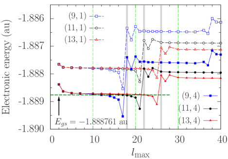
Figure 1: (Color online) Energy of the lowest electronic $X\,^{1}\Sigma_{g}$ state at $R=1.4$ bohr as a function of the $l_{\rm max}$ value used in the Neumann expansion of $1/r_{12}$. The number of $\eta$ points, $n_{\eta}$, and the largest magnetic quantum number, $|m|_{\rm max}$, are labeled as $(n_{\eta},|m|_{\rm max})$. The open symbols correspond to $|m|_{\rm max}=1$, while the filled symbols are for $|m|_{\rm max}=4$. The benchmark energy ($E_{gs}$) from Ref. Sims2006 is shown as well.

VI.2 Convergence of the TDCS

Before we present our results for the cross sections, let us take a closer look at the survival probability

$$P_{\rm surv}=|\langle\Psi_{\rm gs}|\Psi(t)\rangle|^{2}$$ (54)

of the aligned H₂ molecule in its ground state $\Psi_{\rm gs}$. This is shown in Fig. 2. For homonuclear molecules, the independent alignment angle $\theta_{N}$ between the molecular axis and the polarization vector can be confined to the region from $0^{\circ}$ to $90^{\circ}$. In the xuv regime, we observe that the hydrogen molecule shows a larger probability of being ionized or excited (i.e., a lower probability of staying in the initial state) at the end of the pulse in an aligned geometry. This indicates that the perpendicular component of the temporal electric field exerts more influence on the ionization process due to the larger dipole momentum. Interestingly, at the earlier stages of the time evolution (e.g., $t\lesssim 9$ a.u.), when the ionized wave packet is driven back by the change in direction of the electric field, the tilted molecule has a larger probability of staying in its ground state. This happens near the various minima in $P_{\rm surv}$. However, once the electric field has become sufficiently strong ($t\gtrsim 9$ a.u.), the wave packet is driven out and spread into a larger space. This leads to lower minima in $P_{\rm surv}$ for the tilted molecule.

When the wave packet is driven back to the nuclear region and therefore has a chance to recombine with the H${}_{2}^{+}$ ion, a maximum in $P_{\rm surv}$ appears. Not surprisingly, the parallel geometry always has the largest probability for this to happen. Although the wave packet can also be scattered for the untilted molecule in the plane perpendicular to the molecular axis, the probability is undoubtedly larger if the laser electric field is perpendicular to the molecular axis. A similar behavior of H${}_{2}^{+}$ in xuv pulses was observed in Ref. Hu2009 .

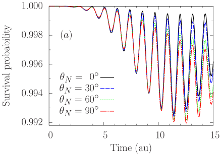
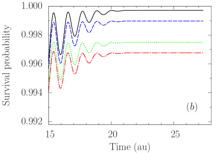
Figure 2: (Color online) Survival probability of the hydrogen molecule subjected to a sine-squared laser pulse with a peak intensity of $10^{15}$ W/cm². The laser pulse lasts for $10$ optical cycles and the system is followed for a period of another $2$ cycles of field-free propagation. The central photon energy of the laser pulse is $75$ eV.

For most calculations performed in this study, we expose the hydrogen molecule to a laser pulse with a peak intensity of $10^{15}$ W/cm². Looking at Fig. 2 we see that the depletion of the initial ground state can be safely neglected for our typical interaction times. Even for $\theta_{N}=90^{\circ}$, $P_{\rm surv}=0.99677$ remains very close to unity. The negligible depletion of the ground state suggests that the concept of cross sections is valid and applicable. On the other hand, it also presents a numerical challenge to predict the cross sections accurately from a time-dependent treatment, due to the generally small ionization probability.

At first glance, a peak intensity of $10^{15}$ W/cm² might seem very intense for most atomic and molecular targets. Here, however, we consider an xuv rather than an IR pulse. For an xuv pulse with central photon energy of $75$ eV, such laser fields definitely fall into the “weak-field” regime. The ponderomotive energy in the xuv regime is much smaller than the photon energy of interest.

Table 1: The discretization and expansion parameters of the H₂ wave function in prolate spheroidal coordinates. Here $\xi_{b}$ stands for the border between the inner and outer regions in the $\xi$ coordinate, while $\xi_{\rm max}$ is the size of the $\xi$ box. In addition, $n_{\xi}$ denotes the number of $\xi$ mesh points in each element. The numbers of $\xi$ elements in the inner and outer region are $n_{\rm inn}$ and $n_{\rm out}$, respectively. These $\xi$ parameters produce the total number of $\xi$ mesh points $N_{\xi}$. The $\xi$ grid I and $\xi$ grid II are used to examine the convergence of our results.

	$\xi_{b}$	$n_{\rm inn}$	$n_{\rm out}$	$\xi_{\rm max}$	$n_{\xi}$	$N_{\xi}$
$\xi$ grid I	$5$	$5$	$67$	$150$	$5$	$288$
$\xi$ grid II	$9$	$1$	$11$	$97$	$14$	$156$

In this work, we are mainly interested in the triple-differential cross section, since it reveals the fine details of possible energy sharings and preferred directions of the ejected electrons in the double-ionization process. Given the discrepancies between results from various calculations found in the literature, we carried out comprehensive convergence tests for our predictions of the TDCSs. These tests are essentially divided into two groups. The first group concerns the laser parameters, while the second one deals with the discretization and expansion parameters. An example of two different parameter sets for the $\xi$ grid is given in Table 1 and will be further discussed below.

In order to obtain a good handle on the sensitivity of the results to the various parameters and the resulting level of “convergence”, we try to only vary a single parameter while keeping all others fixed if possible. For the dependence on the laser parameters, we use the $\xi$ grid I combined with $(n_{\eta},|m|_{\rm max},l_{\rm max})=(9,4,10)$. For the tests regarding the discretizations and expansions, the peak intensity of laser was fixed at $10^{15}$ W/cm² and a time scale of “$10+2$” optical cycles (o.c.) was used. Here “$10+2$” refers to a $10$-cycle laser pulse with a sine-squared envelope for the field amplitude, followed by a $2$-cycle field-free propagation.

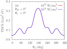
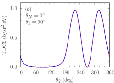
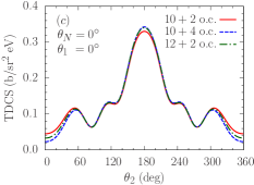
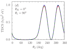
Figure 3: (Color online) Convergence of the coplanar TDCS results for the hydrogen molecule for asymmetric energy sharing with respect to the laser peak intensity and the time scale. The central photon energy is $75$ eV. The slow reference electron, observed at the fixed angle $\theta_{1}$, takes away $20\%$ of the available excess energy $(E_{1}=4.7$ eV), while the other electron takes $80\%$ of $E_{\rm exc}$ $(E_{2}=18.9$ eV). The peak laser intensity in panels $(b)$-$(d)$ is $10^{15}$ W/cm². The two columns show the corresponding convergence of the TDCS for $\theta_{1}=0^{\circ}$ (left) and $\theta_{1}=90^{\circ}$ (right), respectively. $1$ barn (b) $=10^{-24}$ cm².

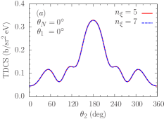
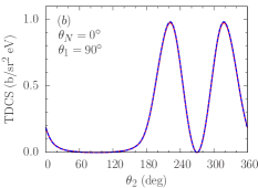
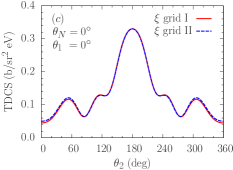
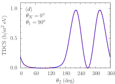
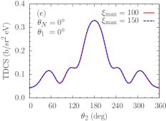
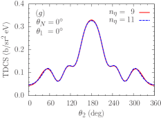
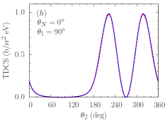
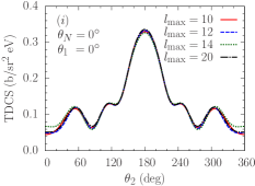
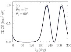
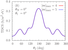
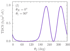
Figure 4: (Color online) Same as Fig. 3, but for the convergence of the TDCS results with respect to the discretization and expansion parameters. See text for the details.

Figures 3 and 4 show the convergence pattern of our TDCS results for asymmetric energy sharing in the parallel geometry ($\theta_{N}=0^{\circ}$). The energy sharing between electron $1$ (observed at the fixed angle $\theta_{1}$) and electron $2$ (observed at the variable angle $\theta_{2}$) is $20\%:80\%$. Only the electron that takes away $20\%$ of the excess energy is recorded at fixed positions either parallel or perpendicular to the polarization axis.

Since the laser pulse is explicitly involved in our time-dependent treatment, we first have to be sure that the extracted cross sections are essentially independent of the laser intensity and the time scales. Only then are the calculations of cross sections meaningful. This also allows us to compare the physical information extracted from our time-dependent scenario to that obtained through conventional time-independent treatments, which are effectively equivalent to the weak-field approximation and “infinitely” long interaction times. Rather than computing the cross sections, it would be more appropriate to consider ionization rates if the cross sections were found to be sensitive to the laser parameters.

In Fig. 3, we display the dependences of our TDCS results upon the laser parameters. Note that the TDCSs extracted from $I_{0}=10^{15}$ W/cm² and $10^{14}$ W/cm² at fixed time evolution of “$10+2$” cycles are nearly identical and agree with each other to better than the thickness of the line. When we turn to the dependence of time scales at a fixed intensity of $10^{15}$ W/cm², we use the same pulse, but allow the system to freely evolve for a few additional cycles to extract the TDCS. This corresponds to the time scale of “$10+4$” o.c. Also, we may increase the laser-molecule interaction time, but extract the TDCSs at the same cycles of field-free time evolution after the pulse died off. This gives the scenario of “$12+2$” o.c. Since the total time durations are the same ($14$ o.c.), they allow us to examine the extracted TDCSs from different perspectives. The increased interaction time yields a reduced bandwidth of the photon energy, while the longer field-free propagation ensures that the double-ionization wave packet is further away from the nuclear region Madsen2007 . The calculated TDCSs indeed show a slight, though in our opinion acceptable, sensitivity to the time scales. Not surprisingly, the sensitivity is most visible for the smaller cross sections, when the two ejected electrons travel nearly parallel along the same direction (c.f. Fig. 3$(c)$).

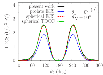
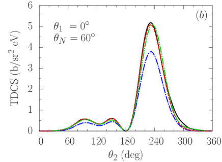
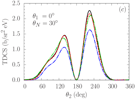
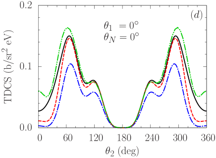
Figure 5: (Color online) Coplanar TDCS of the aligned hydrogen molecule for equal energy sharing ($E_{1}=E_{2}=11.8$ eV). The central photon energy is $75$ eV. One electron is detected at the fixed direction of $\theta_{1}=0^{\circ}$ with respect to the laser polarization axis. Also shown are the one-center spherical ECS results Van2006-1 , the two-center prolate spheroidal results Tao2010 , and one-center spherical TDCC results Colgan2010 .

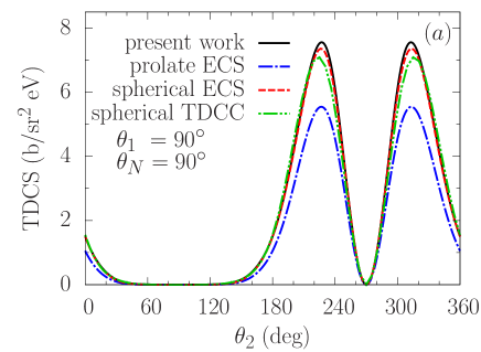
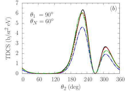
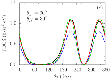
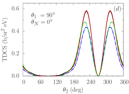
Figure 6: (Color online) Same as Fig. 5, except that the fixed electron is detected at the angle $\theta_{1}=90^{\circ}$ with respect to the laser polarization axis. Since there was a plotting error in Fig. 3 of Tao et al. Tao2010 , we are comparing here with the proper numbers Rescigno2010 from that calculation.

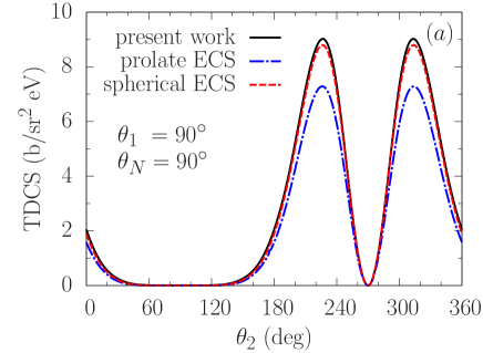
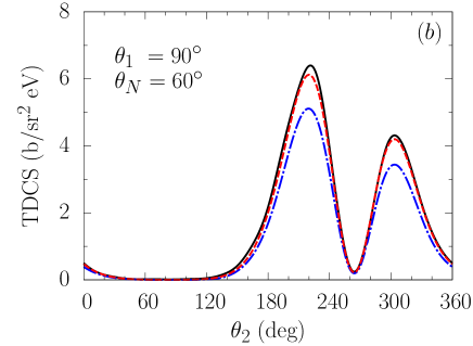
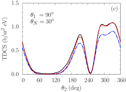
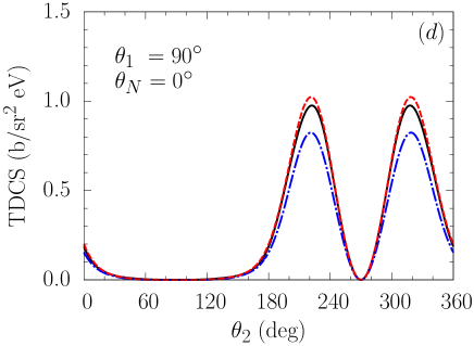
Figure 7: (Color online) Coplanar TDCS of the aligned hydrogen molecule for asymmetric energy sharing. The electron detected at the fixed angle $\theta_{1}=90^{\circ}$ takes away $20\%$ of the available excess energy, while the second electron takes away $80\%$ of $E_{\rm exc}$. The present time-dependent FE-DVR results are compared with those from time-independent one-center spherical ECS Van2006-1 and two-center prolate spheroidal ECS Tao2010 calculations.

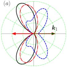
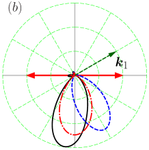
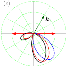
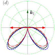
Figure 8: (Color online) Comparison of predicted relative coplanar TDCSs between H₂ in the perpendicular (solid lines) and parallel (dashed lines) geometries, and He (chain lines) Guan2008-2 for equal-energy sharing in polar coordinates. The polarization axis is taken along the horizontal direction. The photon energies for H₂ and He are $75$ eV and $99$ eV, respectively. The fixed observation angles for one of the electrons are $0^{\circ}$ (a), $30^{\circ}$ (b), $60^{\circ}$ (c), and $90^{\circ}$ (d) with respect to the laser polarization vector. Scaling factors were used to emphasize the shape comparison.

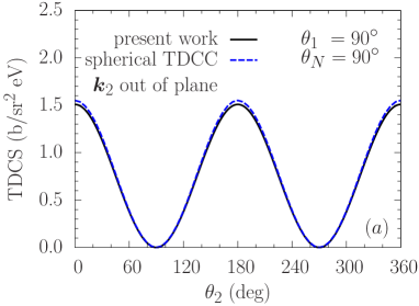
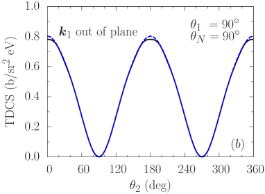
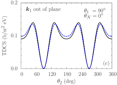
Figure 9: (Color online) Noncoplanar TDCS of the aligned hydrogen molecule for equal energy sharing. The present time-dependent FE-DVR results are compared with TDCC predictions Colgan2010 .

Having confidence in using the current sets of laser parameters, we now turn our attention to the scheme of spatial discretization ($n_{\xi}$, $\xi_{\rm max}$, $n_{\eta}$) and the convergence of the expansion ($l_{\rm max}$, $|m|_{\rm max}$). The results are displayed in Fig. 4.

For the discretization parameters, we obtain well-converged TDCSs by increasing $n_{\xi}$ from $5$ to $7$, $n_{\eta}$ from $9$ to $11$, and extending the spatial box of $\xi_{\rm max}$ from $100$ to $150$. Most importantly, however, we consider two sets of $\xi$ mesh points: $\xi$ grid I and $\xi$ grid II (see Table 1). The principal motivation was to see whether or not we can reproduce the much lower TDCS values (by about $20\%$ compared to the one-center spherical results) that were recently obtained in an ECS calculation in two-center elliptical coordinates by Tao et al. Tao2010 .

We emphasize that these two grids in the “radial” $\xi$ coordinate are completely different regarding both the distribution of the elements and the number of grid points per element. In the $\xi$ grid I, we divide the $\xi$ space into two parts, an inner and an outer region with a border at $\xi_{b}=5$. We place a narrow span of elements in the inner region, and then wider elements in the outer region. In contrast to that, $\xi$ grid II does not distinguish between inner and outer regions, i.e., the elements uniformly span the region from $1$ to $\xi_{\rm max}$. The mesh setup in $\xi$ grid II is the same as that used in Ref. Tao2010 , except for the complex rotation. The $\xi$ grid I has a much denser distribution of mesh points than $\xi$ grid II. Nevertheless, the extracted TDCSs from both sets of $\xi$ grids are in excellent agreement with each other, even for the smallest cross sections. This strongly suggests that the results are well converged at least with regard to the $\xi$ grid. Both $\xi$ sets are good enough to capture the physics of interest. Differences at the $20\%$ level are unlikely to be caused by using different sets of $\xi$ meshes.

Finally, we discuss the convergence of our results with respect to the expansion parameters, $|m|_{\rm max}$ and $l_{\rm max}$. As expected for a one-photon process, $|m|_{\rm max}=4$ produced well-converged results.

Recall the discussion above regarding the ground state, especially how the truncated Neumann expansion of $1/r_{12}$ in our present FE-DVR implementation affects the initial-state energy and therefore the quality of the wave function. For consistency, we use the same $l_{\rm max}$ in the real-time propagation and in the ground-state wave function. As seen from Figs. 4$(i)$ and 4$(j)$, our truncated Neumann expansion has little effect on the calculated TDCS values. Well-converged results can be obtained even with an inappropriately large value of $l_{\rm max}=20$, which yields a slightly higher energy of the ground state (c.f. Fig. 1).

Overall, our detailed convergence tests only reveal a very weak sensitivity of the TDCS results to both the time scales and the values of $l_{\rm max}$. Well-converged TDCS results can be obtained by using either $\xi$ grid I or $\xi$ grid II combined with $(n_{\eta},|m|_{\rm max},l_{\rm max})=(9,4,10)$. In the production calculations for the TDCSs shown in the next subsection, we used the $\xi$ grid I to discretize the two-electron wave packet and a “$10+2$” sine-squared laser pulse with a peak intensity of $10^{15}$ W/cm².

VI.3 TDCSs for the aligned H₂ molecule

Figures 5, 6, and 7 display the coplanar TDCSs of the aligned hydrogen molecule at equal and asymmetric ($E_{1}:E_{2}=20\%:80\%$) energy sharing. The two electrons are detected in the same (coplanar) plane defined by the $\bm{\zeta}$ and $\bm{\epsilon}$ axes. The angles $\theta_{1}$, $\theta_{2}$, and $\theta_{N}$ are all measured with respect to the laser linear polarization axis. We compare our TDCS predictions with those obtained in the time-independent one-center spherical ECS calculation Van2006-1 , the time-independent two-center spheroidal ECS model Tao2010 , and the time-dependent one-center spherical TDCC approach Colgan2010 . The TDCC numbers were recently recalculated with a bigger box size and differ, in some cases substantially, from those published originally Colgan2007 . Except for the recent two-center prolate spheroidal ECS results of Tao et al. Tao2010 ; Rescigno2010 , the agreement between the other three sets of results is very satisfactory. Once again, the largest relative differences occur when the cross sections are small (see Figs. 5$(d)$ and 6$(d)$).

Using spheroidal coordinates as well, as an illustrative example of their two-center ECS approach, Serov and Joulakian Serov2009 recently presented the TDCS at the same photon energy, but only for a single geometry of $\theta_{N}=20^{\circ}$ and $\theta_{1}=40^{\circ}$ for asymmetric energy sharing of $E_{1}:E_{2}=80\%:20\%$. Although not shown here, there is again good agreement between their results, Vanroose et al.’s one-center spherical ECS numbers Van2006-1 , and our time-dependent FE-DVR predictions.

It is also interesting to investigate the dominant escape modes for the various scenarios. These modes are strongly dependent on how the electrons share the excess energy. In an arbitrary geometry ($0^{\circ}\leqslant\theta_{N}\leqslant 90^{\circ}$), for example, the back-to-back escape mode $(\theta_{12}=180^{\circ})$ is forbidden for equal energy sharing. On the other hand, it becomes the dominant mode for significantly asymmetric energy sharing, including the 20%:80% scenario discussed in the present paper (see Fig. 3).

These results can be understood from a symmetry analysis Maulbetsch1995 . Equal-energy sharing and back-to-back emission is equivalent to $\bm{k}_{1}=-\bm{k}_{2}$. When we consider the exchange and parity operations simultaneously in Eq. (V.1), we have $\Phi_{-\bm{k}_{2},-\bm{k}_{1}}=P(-1)^{S}\Phi_{\bm{k}_{1},\bm{k}_{2}}$. Here $P=\pm 1$ is the parity for the gerade and ungerade states, respectively. For the singlet double-continuum state with ungerade parity, we therefore must have $\Phi_{-\bm{k},\bm{k}}(\bm{r}_{1},\bm{r}_{2})=0$ at any configuration of $\bm{r}_{1}$ and $\bm{r}_{2}$. Although the magnitudes of the momenta $k^{\prime}_{1}$ and $k^{\prime}_{2}$ are not exactly conserved in the time-dependent picture, the ionization events we collect must satisfy the condition $k^{\prime}_{1}=k^{\prime}_{2}$ (because of the $\delta$ function in Eq. (53)) for the equal-energy sharing. This is the reason behind the forbidden back-to-back ($\theta_{12}=180^{\circ}$) escape mode for the equal energy sharing, as we observed in Figs. 5 and 6. Since the argument does not involve the relative alignment angles, it is valid for all possible values of $\theta_{N}$. On the other hand, this is not the case when the excess energy is not evenly distributed among the two electrons. Indeed, Figs. 3$(a)$ and 3$(c)$ show maxima in the back-to-back emission, thereby illustrating the dramatic change in the dominant escape mode.

For equal-energy sharing in the parallel geometry ($\theta_{N}=0^{\circ}$), the electron-electron Coulomb repulsion suggests that the TDCS should be dynamically small if the two electrons travel along the same direction. This is in agreement with the numerically small cross sections (not exactly zero, however) at $\theta_{2}=0^{\circ}$ or $360^{\circ}$ seen in Fig. 5$(d)$.

Recall that the one-photon double-photoionization process in helium Colgan2001 ; Guan2008-2 shares the same property. The back-to-back mode is forbidden for equal-energy sharing, and this can be explained by the above argument. It is one of the similarities between the molecular hydrogen and the atomic helium targets for double photoionization. However, Figs. 5, 6, and 7 also reveal significant molecular effects in the TDCS results. These are missing for the helium atom, not only in the shape of the angular distributions, but also in the magnitudes of the cross sections. Depending on the relative orientation $(0^{\circ}<\theta_{N}<90^{\circ})$, there is interference between the $\Sigma_{u}$ and $\Pi_{u}$ symmetries in H₂. A nice example of this effect was presented by Reddish et al. Reddish2008 . Even without interference (i.e., for $\theta_{N}=0^{\circ}$ or $90^{\circ}$), the perpendicular geometry shows much larger magnitudes of the TDCS than the parallel geometry. Figure 8 shows the three cases of angular distributions: H₂ $\bm{\zeta}\perp\bm{\epsilon}$, H₂ $\bm{\zeta}\parallel\bm{\epsilon}$, and He at equal energy sharing. Interestingly, in most cases the angular distributions of the perpendicular geometry resemble those of helium. The molecular effect can definitely not be ignored in the parallel geometry for $\theta_{1}=0^{\circ}$ (c.f. Fig. 8$(a)$). The forward escape mode of the second electron is dominant for the H₂ parallel geometry. In contrast, the backward mode is dominant for the H₂ perpendicular geometry and also for helium.

In Fig. 9, we show the TDCS for noncoplanar geometries. Again, all angles are defined with respect to the polarization vector. For the perpendicular geometry, Fig. 9$(a)$ depicts the escape modes for the configuration of $\bm{k}_{1}\parallel\bm{\zeta}$ (the fixed electron) and at the same time $\bm{k}_{2}$ in the plane perpendicular to the plane formed by $\bm{\epsilon}$ and $\bm{\zeta}$. Figure 9$(b)$ shows the TDCS after exchanging the directions of $\bm{k}_{1}$ and $\bm{k}_{2}$ in Fig. 9$(a)$. With the same directions of $\bm{k}_{1}$ and $\bm{k}_{2}$ as in Fig. 9$(b)$, Fig. 9$(c)$ is for the case of the molecular axis orientated along the polarization vector. In the parallel case ($\theta_{N}=0^{\circ}$), we observe that any escape modes of both electrons ejected in the direction perpendicular to $\bm{\epsilon}$ are forbidden. This can be understood by analyzing the spheroidal harmonics in Eq. (53). In this case, only the ${}^{1}\Sigma_{u}$ states can be populated. Hence, only partial waves with $(m_{1},m_{2})=(-m,m)$ and $(-1)^{\ell_{1}+\ell_{2}}$ can contribute to the cross sections, since ${\cal Y}_{\ell_{1}m_{1}}(k^{\prime},\hat{\bm{k}}_{1}){\cal Y}_{\ell_{2}m_{2}}(k^{\prime},\hat{\bm{k}}_{2})$ at the angles of $\theta_{1}=\theta_{2}=90^{\circ}$ vanish in spherical coordinates. Once again, the agreement between our FE-DVR noncoplanar TDCSs and the refined TDCC results Colgan2010 is excellent.

VII Summary

We have presented calculations for one-photon double ionization of the hydrogen molecule at a photon energy of $75$ eV by solving the time-dependent Schrödinger equation in prolate spheroidal coordinates. The triple-differential cross sections were extracted through the projection of the time-dependent wave packet onto uncorrelated two-electron continuum states, a few cycles of field-free time evolution after the laser pulse died off.

Exhaustive convergence studies of the TDCS results were performed with respect to a number of discretization and expansion parameters, as well as the details of the laser field. These tests provide a strong indication that the results for the triple-differential cross sections presented here are well converged and numerically accurate. Excellent agreement was obtained between the current time-dependent results in prolate spheroidal coordinates, those obtained with the ECS approach in spherical coordinates Van2006-1 and, finally, larger TDCC calculations Colgan2010 than those published earlier Colgan2007 .

The present calculations do not confirm the significant reduction by about $20\%$ in the TDCS results predicted in recent ECS calculations in the two-center prolate spheroidal coordinates Tao2010 . Furthermore, our results did not show the level of sensitivity to the description of the ground state that was also reported by Tao et al. Tao2010 .

The detailed analysis reported in this study provides a high level of confidence in the present results. We hope that they will be used as benchmarks for comparison in future investigations. Tables of these results are available in electronic format from the authors upon request.

References

- (1) H. Bräuning, R. Dörner, C. L. Cocke, M. H. Prior, B. Krässig, A. S. Kheifets, I. Bray, A. Bräuning-Demian, K. Carnes, S. Dreuil, V. Mergel, P. Richard, J. Ullrich, and H. Schmidt-Böcking, J. Phys. B 31, 5149 (1998).
- (2) Th. Weber, A. Czasch, O. Jagutzki, A. Müller, V. Mergel, A. Kheifets, J. Feagin, E. Rotenberg, G. Meigs, M. H. Prior, S. Daveau, A. L. Landers, C. L. Cocke, T. Osipov, H. Schmidt-Böcking, and R. Dörner, Phys. Rev. Lett. 92 163001 (2004).
- (3) T. Weber, A. O. Czasch, O. Jagutzki, A. K. Müller, V. Mergel, A. Kheifets, E. Rotenberg, G. Meigs, M. H. Prior, S. Daveau, A. Landers, C. L. Cocke, T. Osipov, R. Díez Muiño, H. Schmidt-Böcking, and R. Dörner, Nature (London) 431, 437 (2004).
- (4) Th. Weber, PhD. Thesis, Universität Frankfurt (unpublished, 2003).
- (5) M. Gisselbrecht, M. Lavollée, A. Huetz, P. Bolognesi, L. Avaldi, D. P. Seccombe, and T. J. Reddish, Phys. Rev. Lett. 96, 153002 (2006).
- (6) Y. H. Jiang, A. Rudenko, E. Plésiat, L. Foucar, M. Kurka, K. U. Kühnel, Th. Ergler, J. F. Pérez-Torres, F. Martín, O. Herrwerth, M. Lezius, M. F. Kling, J. Titze, T. Jahnke, R. Dörner, J. L. Sanz-Vicario, M. Schöffler, J. van Tilborg, A. Belkacem, K. Ueda, T. J. M. Zouros, S. Düsterer, R. Treusch, C. D. Schröter, R. Moshammer, and J. Ullrich, Phys. Rev. A 81, 021401(R) (2010).
- (7) J. P. Wightman, S. Cvejanović, and T. J. Reddish, J. Phys. B 31, 1753 (1998).
- (8) A. S. Kheifets, Phys. Rev. A 71, 022704 (2005).
- (9) A. S. Kheifets and I. Bray, Phys. Rev. A 72, 022703 (2005).
- (10) W. Vanroose, F. Martín, T. N. Rescigno, and C. W. McCurdy, Phys. Rev. A 70, 050703(R) (2004).
- (11) W. Vanroose, D. A. Horner, F. Martín, T. N. Rescigno, and C. W. McCurdy, Phys. Rev. A 74, 052702 (2006).
- (12) W. Vanroose, F. Martín, T. N. Rescigno, and C. W. McCurdy, Science 310, 1787 (2006).
- (13) J. Colgan, M. S. Pindzola, and F. Robicheaux, Phys. Rev. Lett. 98, 153001 (2007).
- (14) J. Colgan, private communication (2010).
- (15) L. Tao, C. W. McCurdy, and T. N. Rescigno, Phys. Rev. A 82, 023423 (2010).
- (16) D. R. Bates, U. Öpik, and G. Poots, Proc. Phys. Soc. A 66, 1113 (1953).
- (17) S. Barmaki, S. Laulan, H. Bachau, and M. Ghalim, J. Phys. B 36, 817 (2003).
- (18) S. Barmaki, H. Bachau, and M. Ghalim, Phys. Rev. A 69, 043403 (2004).
- (19) Y. V. Vanne and A. Saenz, J. Phys. B 37, 4101 (2004).
- (20) G. Lagmago Kamta and A. D. Bandrauk, Phys. Rev. A 71, 053407 (2005).
- (21) L. Tao, C. W. McCurdy, and T. N. Rescigno, Phys. Rev. A 79, 012719 (2009).
- (22) T. J. Park and J. C. Light, J. Chem. Phys. 85, 5870 (1986).
- (23) D. J. Tannor, in Introduction to Quantum Mechanics, A Time-dependent Perspective, Chap. 11, p318 (University Science Books, Sausalito, California 2007).
- (24) X. Guan, K. Bartschat, and B. I. Schneider, Phys. Rev. A 82, 041404(R) (2010).
- (25) X. Guan, B. Li, and K. T. Taylor, J. Phys. B 36, 3569 (2003).
- (26) P. M. Morse and H. Feshbach, in Methods of Theoretical Physics, Parts I and II (McGraw-Hill, 1953).
- (27) I. A. Stegun, in Handbook of Mathematical Functions with Formulas, Graphs, Mathematical Tables, Chap. 8, p331, eds. M. Abramowitz and I. A. Stegun (1964).
- (28) E. L. Mehler and K. Ruedenberg, J. Chem. Phys. 50, 2575 (1969).
- (29) C. W. McCurdy, M. Baertschy, and T. N. Rescigno, J. Phys. B 37, R137 (2004).
- (30) X. Guan, K. Bartschat, and B. I. Schneider, Phys. Rev. A 77, 043421 (2008).
- (31) X. Guan, C. J. Noble, O. Zatsarinny, K. Bartschat, and B. I. Schneider, Comp. Phys. Comm. 180, 2401 (2009).
- (32) K. T. Taylor, J. S. Parker, D. Dundas, K. J. Meharg, L. R. Moore, E. S. Smyth, and J. F. McCann, in Many-Particle Quantum Dynamics in Atomic and Molecular Fragmentation, Chap. 9, p153, eds. J. Ullrich and V. Shevelko (Springer-Verlag, Berlin Heidelberg 2003).
- (33) C. Flammer, in Spheroidal Wave Functions, (Dover Publications, Inc., Mineola, New York 2005).
- (34) J. Colgan, M. S. Pindzola, and Robicheaux, J. Phys. B 34, L457 (2001).
- (35) L. A. A. Nikolopoulos and P. Lambropoulos, Phys. Rev. A 74, 063410 (2006).
- (36) J. Sims and S. Hagstrom, J. Chem. Phys. 124, 094101 (2006).
- (37) S. X. Hu, L. A. Collins, and B. I. Schneider, Phys. Rev. A 80, 023426 (2009).
- (38) L. B. Madsen, L. A. A. Nikolopoulos, T. K. Kjeldsen, and J. Fernández, Phys. Rev. A 76, 063407 (2007).
- (39) T. N. Rescigno, private communication (2010).
- (40) V. V. Serov and B. B. Joulakian, Phys. Rev. A 80, 062713 (2009).
- (41) F. Maulbetsch and J. S. Briggs, J. Phys. B 28, 551 (1995).
- (42) X. Guan, unpublished (2008).
- (43) T. J. Reddish, J. Colgan, P. Bolognesi, L. Avaldi, M. Gisselbrecht, M. Lavollée, M. S. Pindzola, and A. Huetz, Phys. Rev. Lett. 100, 193001 (2008).