Infall and outflow motions in the high-mass star forming complex G9.62+0.19

Abstract

We present the results of a high resolution study with the Submillimeter Array towards the massive star forming complex G9.62+0.19. Three sub-mm cores are detected in this region. The masses are 13, 30 and 165 M_☉ for the northern, middle and southern dust cores, respectively. Infall motions are found with HCN (4-3) and CS (7-6) lines at the middle core (G9.62+0.19 E). The infall rate is $4.3\times 10^{-3}~{}M_{\odot}\cdot$yr^-1. In the southern core, a bipolar-outflow with a total mass about 26 M_☉ and a mass-loss rate of $3.6\times 10^{-5}~{}M_{\odot}\cdot$yr^-1 is revealed in SO ($8_{7}-7_{7}$) line wing emission. CS (7-6) and HCN (4-3) lines trace higher velocity gas than SO ($8_{7}-7_{7}$). G9.62+0.19 F is confirmed to be the driving source of the outflow. We also analyze the abundances of CS, SO and HCN along the redshifted outflow lobes. The mass-velocity diagrams of the outflow lobes can be well fitted by a single power law. The evolutionary sequence of the cm/mm cores in this region are also analyzed. The results support that UC Hii regions have a higher blue excess than their precursors.

1 Introduction

High-mass stars play a major role in the evolution of the Galaxy. They are the principal sources of heavy elements and UV radiation (Zinnecker & Yorke, 2007). However, the formation and evolution of high-mass stars are still unclear. A possible evolution sequence of high-mass stars from infrared dark clouds to classic Hii regions has been suggested (Van der Tak & Menten, 2005). But one of the major topics whether high-mass stars form through accretion-disk-outflow, like low-mass ones (Shu, Adams & Lizano, 1987), or form via collision-coalescence (Wolfire, & Cassinelli, 1987; Bonnell et al., 1998) is still far from solved.

Yet more and more observations at various resolutions seem to support the accretion-disk-outflow models rather than collision-coalescence models. Disks are detected in several high-mass star forming regions (Patel et al., 2005; Jiang et al., 2005; Sridharan, Williams, & Fuller, 2005). Outflows are found with a high detection rate as in low-mass cores in single-dish surveys (Wu et al., 2004; Zhang et al., 2005; Qin et al., 2008a). High resolution studies have also confirmed that molecular outflows are common in high-mass star forming regions (Su, Zhang, & Lim, 2004; Qiu et al., 2007; Qin et al., 2008b, c; Qiu et al., 2009). Searching for inflow motions also has made large progress in recent years (Wu & Evans, 2003; Fuller, Williams, & Sridharan, 2005; Wyrowski et al., 2006; Klaassen, & Wilson, 2007; Wu et al., 2007, 2009; Furuya, Cesaroni, & Shinnaga, 2011). Both infall and outflow motions in the massive core JCMT 18354-0649S are detected (Wu et al., 2005), and further confirmed by higher resolution observations (Liu et al., 2011). Although accretion-disk-outflow systems are found in high-mass star forming regions, there may be differences between low- and high-mass formation.

The infall motion can be detected via ”blue profile”, a double-peaked profile with the blueshifted peak being stronger for optically thick lines and a single peak at the absorption part of optically thick lines for optically thin lines, which is caused by self absorption of the cooler outer infalling gas towards the warmer central region (Zhou et al., 1993). In contrast, the ”red profile” where the redshifted peak of a double-peaked profile being stronger for optically thick lines is suggested as indicators for outflow motions. Mardones et al. (1997) defined the ”blue excess” in a survey, E, as E = (N_B-N_R)/N_T (Mardones et al. 1997), where N_T is number of sources, N_B and N_R mark the number of sources with blue and red profiles, respectively. The blue excess seems to be no significant differences among the low-mass cores in different evolutionary phases. However, using the IRAM 30 m telescope, Wu et al. (2007) found that UC Hii regions show a higher blue excess than their precursors, indicating fundamental differences between low- and high-mass-star forming conditions. The searches need to be expanded.

Located at a distance of 5.7 kpc (Hofner et al., 1994), G9.62+0.19 is a well studied high-mass star forming region containing a cluster of Hii regions, which are probably at different evolutionary stages. Multiwavelength VLA observations have identified nine radio continuum sources (denoted from A-I) (Garay et al., 1993; Testi et al., 2000), and components C-I are very compact ($<5\arcsec$ in diameter) (Garay et al., 1993; Testi et al., 2000). As revealed in NH₃ (4,4), (5,5) and CH₃CN (J=6-5), component F is a hot molecular core (HMC) and hence likely the youngest source in the region (Cesaroni et al., 1994; Hofner et al., 1994, 1996b). G9.62+0.19 E is a young massive star surrounded by a very small UC Hii region and a dusty envelope (Hofner et al., 1996b), while G9.62+0.19 D a small cometary UC Hii region excited by a B0.5 ZAMS star (Hofner et al., 1996b; Testi et al., 2000). Both G9.62+0.19 E and G9.62+0.19 D seem to be at a more evolved stage than G9.62+0.19 F. Thus G9.62 complex is an ideal sample to examine massive star forming activities including outflow and infall motions.

Maser emissions of NH₃, H₂O, OH, and CH₃OH, as well as the strong thermal NH₃ emissions were detected along a narrow region with projected length $20\arcsec$ and width$\leq 2\arcsec$ (Hofner et al., 1994). A possible explanation for this alignment is compression of the molecular gas by shock front originating from an even more evolved Hii region to the west of the star-forming front (Hofner et al., 1994). High-velocity molecular outflows also have been detected in this region, and G9.62+0.19 F is believed to be the driving source (Gibb, Wyrowski, & Mundy , 2004; Hofner, Wiesemeyer, & Henning , 2001; Su et al., 2005). However, most of previous work was carried out at low frequencies, probing low excitation conditions. To exam the hot dust/gas environment and dynamical processes in this region, higher resolution studies at high frequencies are needed. In this paper we report the results of the Submillimeter Array (SMA) observations toward G9.62+0.19 region at 860 $\micron$.

2 Observations

The observations of G9.62+0.19 with the SMA were carried out on July 9th, 2005 with seven antennas in its compact configuration at 343 GHz for the lower sideband (LSB) and 353 GHz for the upper sideband (USB). The T_sys ranges from 210 to 990 K with a typical value of 380 K at both sidebands during the observations. The observations had two fields for the G9.62+0.19 complex to cover the entire region with emissions. One phase reference center was RA(J2000) = 18^h06^m14.21^s and DEC(J2000) = -$20\arcdeg 31\arcmin 46.2\arcsec$, and the other was RA(J2000) = 18^h06^m15.00^s and DEC(J2000) = -$20\arcdeg 31\arcmin 34.20\arcsec$. Uranus and Neptune were observed for antenna-based bandpass calibration. QSOs 1743-038 and 1911-201 were employed for antenna-based gain correction. Neptune was used for flux-density calibration. The frequency spacing across the spectra band was 0.8125 MHz, corresponding to a velocity resolution of $\sim$0.7 km s^-1.

MIRIAD was employed for calibration and imaging (Sault et al., 1995). The imaging was done to each field separately and the mosaic continuum map was made using a linear mosaicing algorithm (task ”linmos” in MIRIAD). The 860 $\micron$ continuum data was acquired by averaging over all the line-free channels in both sidebands. The spectral cubes were constructed using the continuum-subtracted spectral channels smoothed into a velocity resolution of 1 km s^-1. Additional self-calibration with models of the clean components from previous imaging process was performed on the continuum data in order to remove residual errors due to phase and amplitude problems, and the gain solutions obtained from the continuum data were applied to the line data. The synthesized beam size of the continuum emission with robust weighting of 0.5 is $2.76\arcsec\times 1.88\arcsec$ (P.A.=$21.4\arcdeg$).

3 Results

3.1 Continuum emission

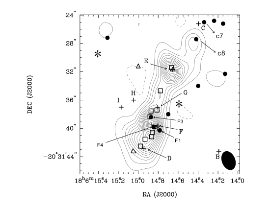
Figure 1: The 860 $\micron$ continuum emission image. The contour levels are from 0.03 Jy beam^-1 (3$\sigma$) in steps of 0.06 Jy beam^-1 (6$\sigma$). The known cm and mm continuum components (Testi et al., 2000) of B, C, D, E, F, G, H, and I are marked by plus signs. Water masers (Hofner, & Churchwell, 1996a) are marked by open squares and methanol masers (Norris et al., 1993) by triangles. The near-IR sources (Persi et al., 2003; Testi et al., 1998; Linz et al., 2005) are marked by filled circles. IRAC sources are marked with asterisks.

The 860 $\micron$ continuum image combining the visibility data from both sidebands is shown in Figure 1 . Three sub-mm cores are detected. The known cm and mm continuum components (Testi et al., 2000) of B, C, D, E, F, G, H, and I are marked by plus signs. Water masers (Hofner, & Churchwell, 1996a) are marked by open squares and methanol masers (Norris et al., 1993) by triangles. The near-IR sources (Persi et al., 2003; Testi et al., 1998; Linz et al., 2005) are marked by filled circles. IRAC sources are taken from the database of Galactic Legacy Infrared Mid-Plane Survey Extraordinaire (GLIMPSE) and labeled with asterisks. The northern core is located at south-east of G9.62+0.19 C, and the middle core is associated with G9.62+0.19 E. The 860 $\micron$ continuum emission at the southern core is concentrated on the hot molecular core G9.62+0.19 F and extends to G9.62+0.19 D in the south and to G9.62+0.19 G in the north.

Gaussian fits were made to the continuum. The northern core seems to be a point-like source. The middle core is very compact with a deconvolved size of $\sim 1.4\arcsec$. The southern core is found to be elongated from north to south with an average size of $2.4\arcsec$, containing at least three sources, D, F, and G. F is at its peak position. The peak positions, sizes, peak intensities and total fluxes of these three sub-mm cores are listed in Column 2-5 in Table 1. The physical properties of these cores will be further discussed in section 4.2.

3.2 Line emission

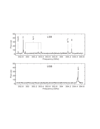
Figure 2: The full LSB and USB spectra in the UV domain over the shortest baseline. The strongest lines are identified and labeled on the plots.

Tens of molecular transitions including hot molecular lines CH₃OH, HCOOCH₃, and CH₃OCH₃ are detected toward both the middle and southern sub-mm cores, indicating these two cores are hot and dense (Qin et al., 2010). Figure 2 presents the full LSB and USB spectra in the UV domain over the shortest baseline. The strongest lines are identified and labeled on the plots. Only HCN (4-3) and CS (7-6) line emissions are detected towards the northern core with our sensitivity. Thus we mainly focus on the middle and southern cores in this paper. The systemic velocities of 2.1 km s^-1 for the middle core and 5.2 km s^-1 for the southern core are obtained by averaging the V_lsr of multiple singly peaked lines. Six transitions of the thioformaldehyde (H₂CS) and molecular transitions SO ($8_{7}$-7₇), CS (7-6), HC¹⁵N (4-3) and HCN (4-3) are analyzed here, while the others will be discussed in another paper. We have made gaussian fits to the beam-averaged spectra, and present the observed parameters of these lines in Table 2.

3.2.1 Line emission at the middle sub-mm core

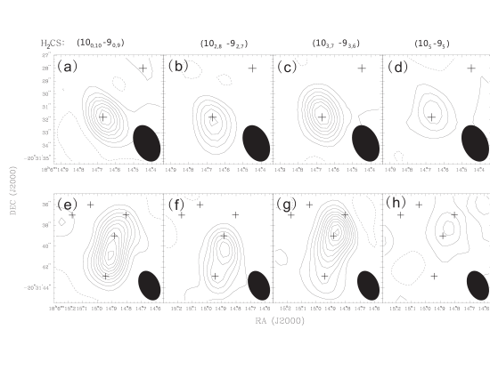
Figure 3: Integrated intensity maps of four transitions of H₂CS at the middle (upper panels) and southern cores (lower panels). The known cm and mm continuum components are marked by plus signs as in the continuum map. The contour levels in all the panels are from 3$\sigma$ in steps of 3$\sigma$. The rms levels are 0.3, 0.3, 0.3 and 0.2 Jy beam${}^{-1}\cdot$km s^-1 for H₂CS (10_0,10-9_0,9) in panels (a) and (e), H₂CS (10_2,8-9_2,7) in panels (b) and (f), H₂CS (10_3,7-9_3,6) in panels (c) and (g), and H₂CS (10₅-9₅) in panels (d) and (h), respectively.

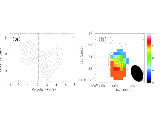
Figure 4: The P-V diagram (left) and First moment map (right) of H₂CS (10_2,8-9_2,7) emission at the middle core. (a) The contours of the P-V diagram are from 0.6 to 1.4 in steps of 0.2 Jy beam^-1 (1$\sigma$). (b) contour plot of H₂CS (10_2,8-9_2,7) integrated intensity image overlayed on the first moment map. The contours are from 0.9 (3$\sigma$) in steps of 0.9 Jy beam${}^{-1}\cdot$km s^-1. The First moment map is constructed from the data after imposing a cutoff of 3$\sigma$.

The integrated intensity maps of four transitions of H₂CS towards the middle core are shown in the upper panels of Figure 3. From (a) to (d), the upper level energy of H₂CS transitions varies from $\sim 90$ K to $\sim 400$ K. The H₂CS emission is spatially coincident with continuum emission of the middle core very well. The Position-Velocity (P-V) diagram and first moment map of H₂CS (10_2,8-9_2,7) emission are presented in Figure 4. The P-V diagram is constructed across the peak of the continuum along the N-S direction. From P-V diagram two emission peaks are clearly revealed. The velocities of the two emission peaks are at 1 and 3 km s^-1 with $1.5\arcsec$ spatial separation, indicating a velocity gradient in N-S direction. The first moment map also shows velocity changes in N-S direction. The small velocity gradient detected in H₂CS (10_2,8-9_2,7) emission may indicate a disk with a low inclination along the line of sight, which requires further confirmation with higher angular resolution observations and other molecular line tracers.

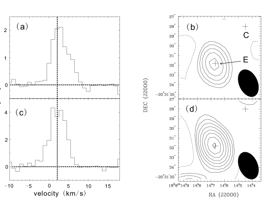
Figure 5: Spectra and integrated intensity maps of HC¹⁵N (4-3) (upper panels) and SO ($8_{7}-7_{7}$) (lower panels) at the middle core. The systemic velocity is marked with the thick vertical dashed lines at the spectra panels. The known cm and mm continuum components of C, and E are marked by plus signs at the integrated maps as the continuum map. (a) the beam-averaged spectrum of HC¹⁵N (4-3) at E, (b) the integrated intensity map of HC¹⁵N (4-3). The contour levels are -1.2 (6$\sigma$), 1.2, 2.4, 4.2, 6.6, 9.6 Jy beam${}^{-1}\cdot$km s^-1, (c) the beam-averaged spectrum of SO ($8_{7}-7_{7}$) at E. (d) the integrated intensity map of SO ($8_{7}-7_{7}$). The contour levels are -1.2 (6$\sigma$), 1.2, 2.4, 4.2, 6.6, 9.6, 13.2, 17.4, 22.2 Jy beam${}^{-1}\cdot$km s^-1.

The spectra and integrated intensity maps of HC¹⁵N (4-3) and SO ($8_{7}$-7₇) are presented in Figure 5. The two spectra seem to be symmetric, and their cores are associated with that of the continuum emission very well.

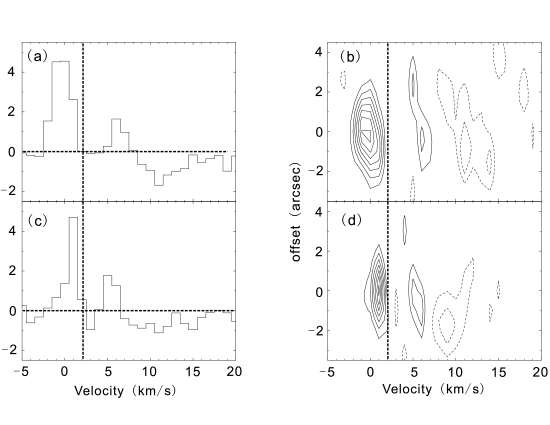
Figure 6: Beam-averaged spectra and Position-Velocity (P-V) diagrams of HCN (4-3) (upper panels) and CS (7-6) (lower panels) at the middle core. The P-V diagrams are cut along a position angle of 0$\arcdeg$. (a) the beam-averaged spectrum of HCN (4-3) at E, (b) the P-V diagram of HCN (4-3). The contour levels are -1.5 (5$\sigma$), -0.9, 0.9, 1.5, 2.1, 2.7, 3,3, 3.9, 4.5 Jy beam^-1, (c) the beam-averaged spectrum of CS (7-6) at E. (d) the P-V diagram of CS (7-6). The contour levels are -1.5 (5$\sigma$), -0.9, 0.9, 1.5, 2.1, 2.7, 3,3, 3.9, 4.5 Jy beam^-1.

Figure 6 presents the spectra and P-V diagrams of HCN (4-3) and CS (7-6) emissions of the middle core. HCN (4-3) and CS (7-6) show asymmetric profile. The blue and red emission peaks of HCN (4-3) are around 0 km s^-1 and 6 km s^-1, respectively. The blueshifted emission of CS (7-6) peaks around 1 km s^-1, while the redshifted around 4 km s^-1. We can see the blueshifted emission of both HCN (4-3) and CS (3-2) is always stronger than the redshifted emission and the absorption is also redshifted, which are blue profiles (see Sect. 1). Besides the ”blue profile”, some weak absorption dips are found around 10 km s^-1 in both the spectra and P-V diagrams of HCN (4-3) and CS (7-6), and further observations are needed to determine the properties of these absorption dips. In this paper we only pay attention to the ”blue-profile” found in CS (7-6) and HCN (4-3) emission.

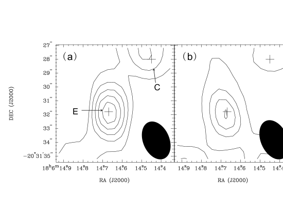
Figure 7: Integrated intensity maps of HCN (4-3) (left) and CS (7-6) (right) at the middle core. The contour levels in both maps are from 1.5 (5$\sigma$) in steps of 3 Jy beam${}^{-1}\cdot$km s^-1. HCN (4-3) is integrated from -3 to 7 km s^-1, while CS (7-6) from -1 to 6 km s^-1

The integrated intensity maps of HCN (4-3) and CS (7-6) towards the middle core are presented in Figure 7. The HCN (4-3) and CS (7-6) are associated with the dust emission.

3.2.2 Line emission at the southern core

The integrated intensity maps of four transitions of H₂CS at the southern core are shown in the lower panels of Figure 3. The upper level energy of H₂CS transitions varies from $\sim 90$ K to $\sim 400$ K from panel (e) to panel (h). As the upper level energy increases, the emission peak of the different transitions of H₂CS moves from S-E to N-W, indicating a temperature gradient in the southern core.

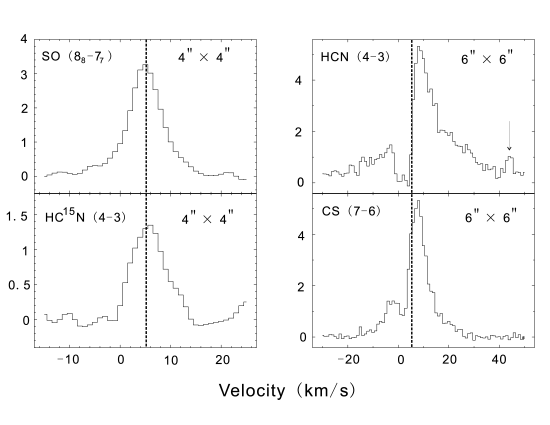
Figure 8: Averaged spectra of SO ($8_{7}-7_{7}$) (upper-left), HC¹⁵N (4-3) (lower-left), HCN (4-3) (upper-right) and CS (7-6) (lower-right) at the southern core. The spectra of SO ($8_{7}-7_{7}$) and HC¹⁵N (4-3) are averaged over a region of 4$\arcsec$, while HCN (4-3) and CS (7-6) are averaged over a region of 6$\arcsec$. HCN $\nu 2=1$ (4-3) emission is marked by the arrow in the upper-right panel, which can be clearly distinguished from the red wing of HCN (4-3).

Averaged spectra of SO ($8_{7}$-7₇), HC¹⁵N (4-3), HCN (4-3) and CS (7-6) at the southern core are presented in Figure 8. The spectra of SO ($8_{7}$-7₇) and HC¹⁵N are averaged over a region of 4$\arcsec$, while HCN (4-3) and CS (7-6) are averaged over a region of 6$\arcsec$. SO ($8_{7}$-7₇) emission has a total velocity extent of larger than 20 km s^-1. From gaussian fit to the spectrum, the peak velocity of SO emission is $5.1\pm 0.1$ km s^-1, coincident very well with the systemic velocity 5.2 km s^-1. HC¹⁵N (4-3) has a velocity extent of about 15 km s^-1. The velocity extents of CS (7-6) and HCN (4-3) are as high as 40 km s^-1 and 60 km s^-1, respectively. Emission wings are clearly detected from the spectra of the four lines. A ”red-profile” is significantly exhibited in the spectra of CS (7-6) and HCN (4-3), of which the redshifted emission is always stronger than the blueshifted emission with an absorption dip at the blueshifted side of the systemic velocity (5.2 km s^-1). This profile is caused by absorption of the colder blueshifted gas in front of the hot core, indicating outflow motions. The ”red-profile” is consistent with that detected using single dish observations (see Figure 6 of Hofner, Wiesemeyer, & Henning (2001)).

The integrated intensity maps of HC¹⁵N (4-3) and SO ($8_{7}$-7₇) at the southern core are presented in Figure 9. To avoid the influence of outflow motions, both the maps are integrated from 2 km s^-1 to 8 km s^-1. Both the emission of HC¹⁵N (4-3) and SO ($8_{7}$-7₇) coincides with the cm/mm component F, and extends from D to G.

As shown in the left panels of Figure 10, the high velocity gas of HC¹⁵N (4-3) and SO ($8_{7}$-7₇) can be identified by the vertically dashed lines in the P-V diagrams. For SO ($8_{7}$-7₇), we integrate from -4 km s^-1 $\leq$ V $\leq$ 0 km s^-1 for the blue wing and 10 km s^-1 $\leq$ V $\leq$ 14 km s^-1 for the red wing, and present the contour map in (c) of Figure 10. For HC¹⁵N (4-3), only the red wing emission is presented in (d) of Figure 10. The high velocity emission of both HC¹⁵N (4-3) and SO ($8_{7}$-7₇) is associated with core F, indicating that core F is the driven source of the outflow. The blue and red wings of SO ($8_{7}$-7₇) overlap to a large extent in the contour maps, and hence the molecular outflow revealed by SO ($8_{7}$-7₇) is observed close to its flow axis.

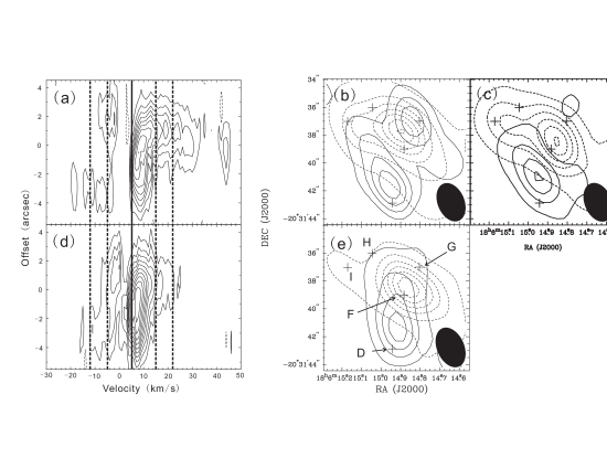
Figure 13: P-V diagrams and integrated intensity maps of HCN (4-3) (upper panels), and CS (7-6) (lower panels) at the southern core. The P-V diagrams are cut along N-S direction. The vertical solid line in P-V diagrams labels the systemic velocity. The dashed and solid contours in the right panels show the red- and blue-shifted emission, respectively. The blue- and red-shifted emission in the integrated maps are integrated from -12 km s^-1 to -5 km s^-1 and 15 km s^-1 to 22 km s^-1, respectively in (b) and (e) panels. (a) P-V diagram of HCN (4-3). The contours are from 0.9 (3$\sigma$) in steps of 1.2 Jy beam^-1. (b) Integrated intensity maps of HCN (4-3) at line wings. The contours are 1.5 (5$\sigma$), 4.5, 7.5, 10.5 Jy beam${}^{-1}\cdot$km s^-1. (c) The integrated intensity maps of HCN (4-3) at extremely high velocities. The blue- and red-shifted emission in the integrated maps are integrated from -20 km s^-1 to -13 km s^-1 and 23 km s^-1 to 39 km s^-1, respectively. The contours are from 1.5 (5$\sigma$) in steps of 3 Jy beam${}^{-1}\cdot$km s^-1 for both blue- and red-shifted emission. (d) P-V diagram of CS (7-6). The contours are from 0.9 (3$\sigma$) in steps of 1.2 Jy beam^-1. (e) Integrated intensity maps of CS (7-6) at line wings. The contours are 1.5 (5$\sigma$), 4.5, 7.5, 10.5 Jy beam${}^{-1}\cdot$km s^-1

Figure 11 presents the channel maps of CS (7-6) emission. The redshifted high-velocity gas seems to be elongated from north-east to south-west, while the blueshifted high-velocity gas from north to south. The high velocity gas revealed by CS (7-6) is also very obvious in the P-V diagram in Figure 13(d). As shown in the P-V diagram, the blueshifted high-velocity gas extends about 8$\arcsec$ from north to south. The high-velocity emission integrated over the wings (-12 km s^-1 $\leq$ V $\leq$ -5 km s^-1 for the blue wing and 15 km s^-1 $\leq$ V $\leq$ 22 km s^-1 for the red wing) is presented in Figure 13(e).

Figure 12 is the channel maps of HCN (4-3) emission. The maximum of absorptions appears at around 0 km s^-1. The redshifted high-velocity gas seems to be elongated from west to east, while the blueshifted high-velocity gas from north to south. At very high velocity channels (V$\leq$ -16 km s^-1), the blueshifted emission is totally located at south-east. By comparing the channel maps and P-V diagrams (see Figure 13) of HCN (4-3) and CS (7-6) at velocity intervals -12 km s^-1 $\leq$ V $\leq$ -5 km s^-1 and 15 km s^-1 $\leq$ V $\leq$ 22 km s^-1, we find similar structures in CS (7-6) and HCN (4-3) emissions. The high-velocity emission of HCN (4-3) integrated from -12 km s^-1 to -5 km s^-1 for the blue wing and from 15 km s^-1 to 22 km s^-1 for the red wing is presented in the panel (b) of Figure 13. As of CS (7-6), the blueshifted gas revealed by HCN (4-3) is elongated from north to south with the emission center located between G9.62+0.19 F and G9.62+0.19 D, while the redshifted gas from north-east to south-west. Two clumps are found in the blueshifted high-velocity emission of HCN (4-3), which locate at north-west and south-east of F, respectively.

In order to reveal the very high velocity emission traced by HCN (4-3) but not CS (7-6), we integrate over the wings at much higher velocities (-20 km s^-1 $\leq$ V $\leq$ -13 km s^-1 for the blue wing and 23 km s^-1 $\leq$ V $\leq$ 39 km s^-1 for the red wing), and present the integrated emission map in Figure 13(c). The redshifted emission is elongated from north-east to south-west with the emission center located between G9.62+0.19 F and G9.62+0.19 G, while the blueshifted emission center located between G9.62+0.19 F and G9.62+0.19 D. It is clearly seen that the high velocity gas traced by SO ($8_{7}$-7₇), CS (7-6) and HCN (4-3) have different spatial distributions, which should be caused by the complicated interactions between the outflow and the ambient gas. It may also indicate a change of the outflow axis. The change of outflow axis is also found in IRAS 20126+4104 (Su et al., 2007) and JCMT 18354-0649S (Liu et al., 2011).

From the integrated emission maps of SO ($8_{7}$-7₇), HCN (4-3) and CS (7-6) high velocity gas, it is clearly seen that G9.62+0.19 F is located at the middle of the redshifted and blueshifted lobes, suggesting G9.62+0.19 F is the outflow driving source.

4 Discussion

4.1 Rotational temperature of H₂CS transitions

Six transitions of H₂CS have been detected in the middle and southern cores, enabling us to estimate the rotational temperature. Under the assumptions that the gas is optically thin under local thermodynamic equilibrium and the gas emission fills the beam, the rotation temperature and beam-averaged column density can be estimated using the Rotational Temperature Diagram (RTD) by (Cummins, Linke, &Thaddeus, 1986; Turner et al., 1991; Liu, et al., 2002)

$$\textrm{ln}(\frac{N_{u}}{g_{u}})=\textrm{ln}(\frac{N_{T}}{Q_{rot}})-\frac{E_{u}}{T_{rot}}=\textrm{ln}[2.04\times 10^{20}\frac{\int~{}I(Jy~{}beam^{-1})dv(km~{}s^{-1})}{\theta_{a}\theta_{b}(arcsec^{2})g_{I}g_{K}\nu^{3}(GHz^{3})S\mu^{2}(debye^{2})}]$$ (1)

where N_u is the observed column density of the upper energy level, g_u is the degeneracy factor in the upper energy level, N_T is the total beam-averaged column density, Q_rot is the rotational partition function, E_u is the upper level energy in K, T_rot is the rotation temperature, $\int$ I dv is the integrated intensity of the specific transition, $\theta_{a}$ and $\theta_{b}$ are the FWHM beam size, g_K is the K-ladder degeneracy, g_I is the degeneracy due to nuclear spin, $\nu$ is the rest frequency, and S is line strength and $\mu$ the permanent dipole moment. For H₂CS, the interchangeable nuclei are spin $\frac{1}{2}$, leading to ortho- and para-forms with g_I equaling $\frac{3}{4}$ and $\frac{1}{4}$, respectively (Blake et al., 1987; Turner et al., 1991). The partition function Q_rot of H₂CS is (Blake et al., 1987)

$$Q_{rot}=2[\frac{\pi(kT_{rot})^{3}}{h^{3}ABC}]^{\frac{1}{2}}$$ (2)

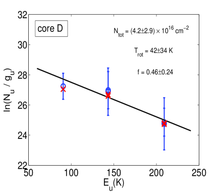
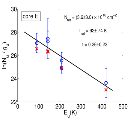
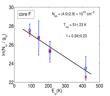
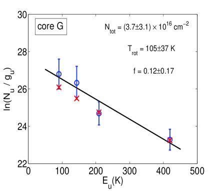
Figure 14: Population diagrams of H₂CS towards four cm/mm cores. The names of the cores are labeled on the upper-right corner of each panel. Open circles in blue represent the observed data. The vertical bars present 3$\sigma$ errors of ln(N_u/g_u) due to the uncertainties of integrated intensities. The solid line shows the linear least-squares fitting using the Rotational Temperature Diagram method. Crosses in red mark the weighted mean results from Population Diagram analysis. The inferred parameters from the Population Diagram analysis are presented on the upper-right corners of each panel.

where k and h are the Boltzmann and Planck constants, respectively, and A, B, and C are the rotation constants. Thus the rotation temperature T_rot and total column density N_T can be estimated by least-squares fitting to the multiple transitions. We applied the RTD method towards D, E, F, G (see Figure 14), and the fitting results are listed in the second and third columns of Table 3. The rotational temperature of the middle core (E) is 83$\pm$21 K. In the southern core, the rotational temperature estimated decreases from G (91 K) to F (83 K) and D (43 K), suggesting the temperature gradient in the southern core. The total column density of H₂CS ranges from 1.3$\times$10¹⁵ (G) to 3.8$\times$10¹⁵ cm^-2 (D).

However, the filling factor and the optical depth correction were not taken account of in the RTD method. To investigate their effect we applied the Population Diagram (PD) analysis (Goldsmith, & Langer, 1999; Wang et al., 2010). In the PD analysis, we have

$$\textrm{ln}(\frac{\hat{N_{u}}}{g_{u}})=\textrm{ln}(\frac{N_{T}}{Q_{rot}})-\frac{E_{u}}{T_{rot}}+\textrm{ln}(f)-\textrm{ln}(\frac{\tau}{1-e^{-\tau}})$$ (3)

where $\hat{N_{u}}$ is the inferred column density of the upper energy level from the PD analysis, f is the source filling factor and $\tau$ is the optical depth. The optical depth $\tau$ can be expressed by (Remijan et al., 2004)

$$\tau=\frac{8\pi^{3}S\mu^{2}\nu}{3k\Delta\textrm{v}T_{rot}}\frac{N_{T}}{Q_{rot}}e^{-\frac{E_{u}}{T_{rot}}}$$ (4)

where $\Delta$v is the FWHM line width. Under LTE, the upper-level populations, $\hat{N_{u}}$, can be predicted according to the right-hand side of Equation (3) for a given set of total column density, N_T, rotational temperature, T_rot, and source filling factor, f. The expected $\hat{N_{u}}$ were evaluated for the parameter space of T_rot = 10-500 K, N_T = 10¹⁴-10¹⁷ cm^-2, and f between 0.01 and 1.0. To compare the observed $N_{u}$ and the inferred $\hat{N_{u}}$, we calculate the $\chi^{2}$ as:

$$\chi^{2}=\sum(\frac{N_{u}-\hat{N_{u}}}{\delta~{}N_{u}})^{2}$$ (5)

where $\delta~{}N_{u}$ is the 1 $\sigma$ error of observed upper-state column density. Although the $\chi^{2}$ is a good representation of the goodness of fit, the parameter set with the lowest $\chi^{2}$ may not actually represent physical parameters very well due to the uncertainties of the observed data. In order to find a representative parameter set, we compute a weighted mean and standard deviation for all the parameters, with the weights being the inverse of the $\chi^{2}$. All the parameter sets where the inferred upper-level population $\hat{N_{u}}$ corresponds with the observed upper-level population $N_{u}$ within 3 $\sigma$ are used to compute the weighted means and standard deviations. The derived rotational temperature, total column density and filling factor of each component are list in the [3-5] columns of Table 3. The inferred optical depths of each line transition are listed in the last six columns of Table 3. The rotational temperatures of D, E, F, G are estimated to be 42$\pm$34, 92$\pm$74, 51$\pm$23 and 105$\pm$37 K, respectively. A temperature gradient in the southern core is also revealed as in the RTD method. The four components D, E, F, G has similar total column densities as high as 4$\times 10^{16}$ cm^-2, about an order of magnitude higher than those obtained from RTD method, which are mainly due to the small source filling factor ($<$0.5). The optical depths of H₂CS (10_0,10-9_0,9) at the four components are all much larger than one, while the other transitions are always optically thin except H₂CS (10_2,9-9_2,8) line at G.

4.2 Core properties

In the optically thin case, the total dust and gas masses of the three sub-mm cores can be obtained with the formula $M=S_{\nu}D^{2}/\kappa_{\nu}RB_{\nu}(T_{d})$ (Hildebrand , 1983), where $S_{\nu}$ is the flux at 860 $\micron$, D is the distance, R=0.01 is the mass ratio of dust to gas, and $\kappa_{\nu}$ is dust opacity per unit dust mass. $B_{\nu}(T_{d})$ is the Planck function at a dust temperature of T_d. We assume that T_d equals the rotational temperature of H₂CS. For the northern core, since only CS (7-6) (upper energy E_u = 65.8 K) and HCN (4-3) (E_u = 42.5 K) exhibit strong emission lines, we assume T_d to be 50 K. Together with the measurements at centimeter and millimeter wavelengths, Su et al. (2005) extrapolated the ionized gas emission at mm/submm wavelengths, and found that the 0.85 mm continuum associated with components D, E, and F are dominated by thermal dust emission. They have derived opacity index $\beta$ of components E and F to be 1.2, and 0.8, respectively. For the northern sub-mm core, ${\beta}=1.5$ is assumed. Using the above dust opacity indexes, we adopt $\kappa_{\nu}$=2.0, 1.8, and 1.5 cm²g^-1 for the northern, middle and southern cores, respectively (Ossenkopf & Henning, 1994). At the distance of 5.7 kpc , we get the total dust and gas masses for these three cores, and list all the parameters in Table 1. The deduced masses for the northern, middle and southern cores are 13, 30, 165 M_☉, respectively. The column density of H₂ are 1.2$\times 10^{24}$ and 2.1$\times 10^{24}$ cm^-2 for the middle and southern sub-mm cores, respectively.

4.3 Infall properties in the middle core

In the middle core, both CS(7-6) and HCN(4-3) emission exhibits ”blue profile” feature, indicating infall motions of the gas envelope toward the central star (Keto, Ho,& Haschick, 1988; Zhou et al., 1993; Zhang, Ho, & Ohashi, 1998; Wu & Evans, 2003; Wu et al., 2005, 2007; Fuller, Williams, & Sridharan, 2005; Wyrowski, 2007; Sun, & Gao, 2008). The velocity difference (0.9 km s^-1) between the absorption dip in CS (7-6) spectrum (3 km s^-1) and the systemic velocity (2.1 km s^-1) is taken as the infall velocity $V_{in}$. Since both HCN (4-3) and CS (7-6) emissions are not resolved towards the middle core, we simply take the dust core size as the radius of the infall region, which may underestimate the infall rate derived below. The kinematic mass infall rate can be calculated using dM/dt=$4{\pi}R_{in}^{2}nmV_{in}$. n=1.5$\times 10^{7}$cm^-3 is the number density of this dust core. Taking Helium into account, the mean molecular mass m is 1.36 times of H₂ molecule mass. The infall rate calculated is $4.3\times 10^{-3}~{}M_{\odot}\cdot$yr^-1. For comparison, the $V_{in}$ from pure free-infall assumption is also derived with the formula $V_{in}^{2}=2GM/R_{in}$. The pure free-infall velocity is $V_{in}=3.6~{}$km s^-1 and thus the ”gravitational” mass infall rate is $1.7\times 10^{-2}~{}M_{\sun}\cdot$yr^-1, which is larger than the kinematic infall rate.

4.4 Outflow properties in the southern core

4.4.1 Shock chemistry in the outflow region of the southern core

Observations have suggested that there are important differences in molecular abundances in different outflow regions (Bachiller et al., 1997; Choi et al., 2004; Jörgensen, Schöier, & van Dishoeck, 2004; Codella et al., 2005). Significant abundance enhancements are found in the shocked region for sulfur-bearing molecules (Bachiller et al., 1997; Jörgensen, Schöier, & van Dishoeck, 2004), and the abundance of HCN in outflow regions is related to atomic carbon abundance (Choi, 2002). However, previous studies of the chemical impact of outflows are confined to the well collimated outflows around Class 0 sources, while such studies especially high resolution studies on massive outflows are rare (Bachiller et al., 1997; Jörgensen, Schöier, & van Dishoeck, 2004; Arce et al., 2007).

A red and bright IRAC source is found to be associated with the southern core. The magnitudes of the IRAC source at 3.6 $\micron$, 4.5 $\micron$ and 5.8 $\micron$ are $10.102\pm 0.093$, $8.361\pm 0.108$ and $7.778\pm 0.302$ mag, respectively. The [3.6-4.5] color is as large as 1.74, indicating shocked emission in the southern core (Takami et al., 2010). Maser emissions of NH₃, H₂O, OH, and CH₃OH, as well as the strong thermal NH₃ emissions also uncover the existence of the shocked gas (Hofner et al., 1994). Outflows can be revealed from shocked H₂ emission probed by the strong and extended emission at the 4.5 $\micron$ band (Qiu et al., 2008; Takami et al., 2010). Thus the massive outflow in the southern core of G9.62 complex provides an ideal sample to study shock chemistry.

The fractional abundance of a certain molecule is defined as $\chi=N_{T}/N_{H_{2}}$, where $N_{T}$ is the total column density of a specific molecule and $N_{H_{2}}$ is the H₂ column density. Assuming that the gas is optically thin and the emission fills the beam, the beam-averaged total column density of a specific molecule can be obtained from:

$$N_{T}=2.04\times 10^{20}\frac{\int~{}I(Jy~{}beam^{-1})dv(km~{}s^{-1})Q_{rot}e^{E_{u}/T_{rot}}}{\theta_{a}\theta_{b}(arcsec^{2})g_{I}g_{K}\nu^{3}(GHz^{3})S\mu^{2}(debye^{2})}$$ (6)

Assuming that T_rot of HC¹⁵N equals to that of H₂CS and the gas is optically thin, $N_{T}$ of HC¹⁵N is calculated to be $3.0\times 10^{13}$ cm^-2 at the core region. At the galactocentric distance of 3 kpc for G9.62+0.19 (Scoville et al.1987,Hofner et al.1994), the abundance ratio [¹⁴N]/[¹⁵N]$~{}\approx~{}350$ (Wilson and Rood. 1994). Thus the total column density of HCN at the core region should be $1.1\times 10^{16}$ cm^-2. Therefore, the fractional abundance of HCN relative to H₂ at the core region is $5.2\times 10^{-9}$. HCN appears to be greatly enhanced in the outflow regions of the L1157 (Bachiller et al., 1997), while has similar abundances in the outflow region and the ambient cloud of NGC 1333 CIRAS 2A (Jörgensen, Schöier, & van Dishoeck, 2004). Owing to the lack of a direct estimation of the H₂ column density towards the outflow region, the fractional abundance of HCN in the outflow region is also assigned to $5.2\times 10^{-9}$ in calculating the outflow parameters. Since the HC¹⁵N emission traces outflowing gas at much lower velocity than HCN, perhaps HCN could be more enhanced in the high velocity component. With the possibility of higher opacity and the lack of direct H₂ column density measurement, the derived fractional abundance perhaps is a lower limit anyway. Su et al. (2007) estimate an HCN abundance of $\sim 1-2\times 10^{-8}$ in the massive outflow lobes of IRAS 20126+4104, which is comparable to our estimation here.

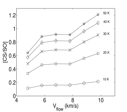
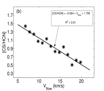
Figure 15: Abundance ratios of [CS/SO] (left) and [CS/HCN] (right) versus flow velocity along the redshifted lobe. We range the excitation temperature from 10 K to 50 K to derive the abundance ratios of [CS/SO]. The excitation temperature in calculation of abundance ratios of [CS/HCN] is assumed to be 30 K. The solid line in the right panel is the linear least-squares fitting, and the fitting results are presented in the upper-right corner.

Since the blueshifted outflow gas traced by CS (7-6) and HCN (4-3) suffers self-absorption, the abundance ratios among SO ($8_{7}-7_{7}$), CS (7-6), and HCN (4-3) were inferred from the beam-averaged spectra taken from the redshifted outflow lobe. The abundance ratio as a function of flow velocity (the outflow velocity relative to the systemic velocity) of [CS/SO] is obtained assuming five different excitation temperatures in the left panel of Figure 15. It can be seen that the abundance ratio of [CS/SO] increases with the excited temperature. At each excitation temperature, the abundance ratio of [CS/SO] has lower values at flow velocities less than 6 km s^-1, and higher values when V_flow larger than 8 km s^-1, whereas the abundance ratio seems to be constant at flow velocities between 6 km s^-1 and 8 km s^-1. There are two reasons for the lower abundance ratio when V${}_{flow}~{}<$ 6 km s^-1: first, the flux missing of CS (7-6) due to the interferometer is more serious than SO ($8_{7}-7_{7}$); second, CS (7-6) may be more optically thick at lower flow velocities than SO ($8_{7}-7_{7}$). As shown in the P-V diagrams, the emission region of CS (7-6) is much larger than SO ($8_{7}-7_{7}$) at high velocities. The higher abundance ratio when V${}_{flow}~{}>$ 8 km s^-1 is due to the smaller filling factor of SO ($8_{7}-7_{7}$) emission. We propose the mean observed value between 6 km s^-1 and 8 km s^-1 can represent the actual abundance ratio of [CS/SO]. Assuming a typical excitation temperature of T_ex=30 K (Wu et al., 2004), the abundance ratio of [CS/SO] at the redshifted lobe is inferred as 0.7. Nilsson et al. (2000) find that the [SO/CS] abundance ratios are strongly enhanced in the Orion A and NGC 2071 outflows where the [SO/CS] ratios are estimated to be about 24 and 2.2, respectively. However, the [SO/CS] abundance ratio in the outflow of G9.62+0.19 is found to be 1.4, much lower than that found in Orion A outflow.

As shown in the right panel of Figure 15, the abundance ratio of [CS/HCN] decreases linearly with the flow velocity. To avoid the missing flux difficulty, the abundance ratio is calculated at high flow velocities larger than 7 km s^-1. The decreasing of the abundance ratio with velocity is because that the emission region traced by CS (7-6) is always smaller than HCN (4-3), leading to smaller filling factor for CS (7-6), which can be verified easily by comparing the channel maps between CS (7-6) in Figure 11 and HCN (4-3) in Figure 12 at high velocities. We fitted the observed data with a linear function, and adopted the value at flow velocity of 10 km s^-1 as the actual abundance ratio of [CS/HCN] in the outflow region, which is [CS/HCN]=1.2. Since HCN fractional abundance is $5.2\times 10^{-9}$, the fractional abundances of CS and SO are deduced to be $6.2\times 10^{-9}$ and $8.9\times 10^{-9}$, respectively.

4.4.2 Properties of the bipolar-outflow traced by SO ($8_{7}-7_{7}$) emission

The SO ($8_{7}-7_{7}$) emission in the southern core shows line wings, suggesting outflow motions. From the integrated intensity map in Figure 10(c), we find the outflow lobes revealed by SO ($8_{7}-7_{7}$) emission peak at different position with different position angle compared with previously reported H₂S ($2_{2,0}-2_{1,1}$) (Gibb, Wyrowski, & Mundy , 2004) and HCO⁺ (1-0) data (Hofner, Wiesemeyer, & Henning , 2001). But in the same sense, the blue- and red-lobes revealed by SO overlap to a large extent as well as HCO⁺ (1-0) and H₂S ($2_{2,0}-2_{1,1}$) data, consistent with the argument of the outflow being viewed pole-on (Hofner, Wiesemeyer, & Henning , 2001).

The total mass of each outflow lobe is given by:

$$M_{flow}=1.04~{}\times~{}10^{-4}D^{2}\frac{Q_{rot}e^{E_{u}/T_{rot}}}{\chi\nu^{3}S\mu^{2}}\int\frac{\tau}{1-e^{-\tau}}S_{\nu}dv$$ (7)

where M_flow, D, S_ν, $\chi$, and $\tau$ are the outflow gas mass in M_☉, source distance in kpc, line flux density in Jy, relative abundance to H₂, and optical depth. The other parameters have the same units as in equation (1). The fractional abundance of SO is taken as $8.9\times 10^{-9}$ (see Sec.4.4.1). Assuming an excitation temperature of 30 K and the outflowing gas is optically thin, the inferred outflow masses are 13 M_☉ for each of red and blueshifted lobes. Thus, the momentum can be calculated by $P=\sum$M(v)dv, and the energy by $E=\sum{\frac{1}{2}}$M(v)v²dv, where $v$ is the flow velocity. The derived parameters are listed in Table 4. The momentum and energy of the red lobe are 82 M${}_{\sun}\cdot$km s^-1 and $5.4\times 10^{45}$ erg. For the blue lobe, the momentum and energy are calculated to be 86 M${}_{\sun}\cdot$km s^-1 and $5.8\times 10^{45}$ erg. The dynamical timescale t_dyn is estimated as R/V_char, where R ($\sim$ 0.06 pc) is adopted as the mean size of the outflow lobes assuming a collimation factor of unity, and V_char ($\sim$ 5.5 km s^-1) is assumed as the mass weighted mean velocity. Thus, the dynamic timescale is estimated to be $1\times 10^{4}$ year, which may be underestimated due to the uncertainty of the outflow scale. The mechanical luminosity L, and the mass-loss rate $\dot{M}$ are calculated as L=E/t, $\dot{M}=P/(tV_{w})$, where the wind velocity V_w is assumed to be 500 km s^-1 (Lamers et al., 1995). The mechanical luminosity L and the total mass-loss rate are estimated to be 9.3 L_☉ and $3.6\times 10^{-5}$ M_☉$\cdot$yr^-1, respectively.

4.4.3 Very high-velocity gas detected in CS (7-6) emission

The CS (7-6) emission at the southern core shows ”red-profile” with wide wings. We take $6.2\times 10^{-9}$ as the fractional abundance of CS relative to H₂ along the outflow lobes. Assuming T_ex = 30 K, we derive the parameters for the CS outflow (Table 4) with the same method used for SO ($8_{7}-7_{7}$). The outflow masses at very high velocities (v${}_{flow}~{}>~{}$10 km s^-1) are 3.7 M_☉ and 5.5 M_☉ for the blueshifted and redshifted lobes, respectively. The momentum and energy of the blueshifted lobe at very high velocities are calculated to be 47 M${}_{\sun}\cdot$km s^-1 and $6.0\times 10^{45}$ erg. For the redshifted lobe, the momentum and energy at extremely high velocities are calculated to be 68 M${}_{\sun}\cdot$km s^-1 and $8.7\times 10^{45}$ erg, which are similar to the blueshifted lobe.

4.4.4 Very high-velocity gas detected in HCN (4-3) emission

As discussed before, HCN (4-3) has a velocity extent of at least 60 km s^-1, which traces extremely high-velocity (EHV) gas. Adopting an excited temperature of 30 K, and an HCN-to-H₂ abundance ratio of $5.2\times 10^{-9}$, the parameters of the outflow are calculated and listed in Table 4. The outflow mass at very high velocities (v${}_{flow}~{}>~{}$10 km s^-1) are 5.2 M_☉ and 17.6 M_☉ for the blueshifted and redshifted lobes, respectively. The momentum and energy of the blueshifted lobe at very high velocities are 85 M${}_{\sun}\cdot$km s^-1 and $1.4\times 10^{46}$ erg. For the redshifted lobe, the momentum and energy at very high velocities are 294 M${}_{\sun}\cdot$km s^-1 and $5.5\times 10^{46}$ erg, which are larger than the blueshifted lobe.

4.4.5 Mass-Velocity diagrams

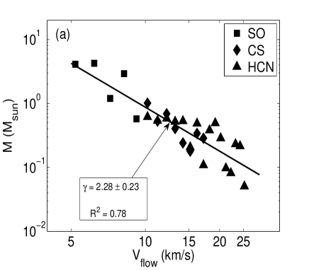
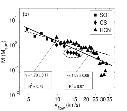
Figure 16: Mass-Velocity relationships for the outflow lobes. Left : blueshifted lobe; right: redshifted lobe. The solid lines in both panels show the power law fit towards all the data. The dashed line in the right panel shows the power law fit towards the HCN and SO data up to V_flow = 25 km s^-1. The fitting results are presented in the lower-left corners.

A broken power law, $dM(v)/dv\propto v^{-\gamma}$ usually exhibits in molecular outflows near young stellar objects (Chandler et al., 1996; Lada, & Fich, 1996; Ridge, & Moore, 2001; Su, Zhang, & Lim, 2004; Qiu et al., 2007, 2009). The slope, $\gamma$, typically ranging from 1 to 3 at low outflow velocities, and often steepens at velocities larger than 10 km s^-1 — with $\gamma$ as large as 10 in some cases (Arce et al., 2007). Assuming optically thin, the mass-velocity diagrams of the outflow at the southern core of G9.62+0.19 complex are shown in Figure 16. SO ($8_{7}-7_{7}$), CS (7-6), HCN (4-3) results were all used in the mass spectra. We calculate the outflow mass traced by CS (7-6) and HCN (4-3) from V_flow of 10 km s^-1 to avoid the absorption of the spectra. Instead of broken power law appearance, the mass-velocity diagram of blueshifted lobe can be well fitted by a single power law with a power indexes of $2.28\pm 0.23$. The mass-velocity diagram of redshifted lobe can be well fitted by a single power law with a power indexes of $1.70\pm 0.17$ even though the mass drops more rapidly after 25 km s^-1. As marked by the dashed ellipse in the right panel, the outflow mass revealed by CS (7-6) is much lower than that revealed by HCN (4-3) at very high velocities. Despite the CS data, the mass-velocity diagram of redshifted lobe at velocities smaller than 25 km s^-1 can be fitted by a single power law with a much smaller power indexes of $1.08\pm 0.09$. However, no significant slope changes are found in both the red- and blue-shifted lobes of the outflow at the southern core, which are very different from those previous works.

4.5 Different evolutionary stages of the three dust cores

The northern core has the smallest diameter and mass among the three cores. It seems likely to be a point source after deconvolution. It is located south of the nominal radio UC Hii region G9.62+0.19 C. In this region, eight near-IR sources are detected in a diffuse near-IR nebulosity at the west of the radio emission peak (Persi et al., 2003). The reddest one c7 (18^h06^m14.34^s,-20$\arcdeg$31$\arcmin$25.0$\arcsec$) is located within $1\arcsec$ of the radio peak, while the faintest one c8 (18^h06^m14.42^s,-20$\arcdeg$31$\arcmin$27.4$\arcsec$) seems to be associated with the sub-mm core detected in SMA observation. Source c8 is too faint to be detected even at H band and also shows no emission at 12.5 $\micron$. In contrast to the bright, rich molecular spectrum forest in the middle and southern sub-mm cores, the northern sub-mm core lacks strong molecular emissions. There is also no other early star forming signature such as masers associated with it. Since it is with near-IR emission and at the edge of the UC Hii region G9.62+0.19 C, the northern core may be just a remnant core in the envelope of UC Hii region G9.62+0.19 C, which needs further observations.

The middle core is associated with the hyper-compact Hii region G9.62+0.19 E (Garay et al., 1993; Kurtz, & Franco, 2002). OH, H₂O, and NH₃ (5,5) masers have been detected near the radio emission peak (Forster & Caswell, 1989; Hofner et al., 1994; Hofner, & Churchwell, 1996a). Periodic class II methanol masers are also found in G9.62+0.19 E (van der Walt, Goedhart, & Gaylard, 2009; Goedhart, Gaylard, & van der Walt, 2005; Norris et al., 1993). Methanol masers are believed to be a good tracer of young massive star forming regions at stages earlier than relatively evolved UC Hii regions (Longmore et al., 2007). No infrared source coincides with G9.62+0.19 E (Persi et al., 2003). Hot molecular CH₃CN lines are detected in this region, and a kinematic temperature of T_k = 108 K was obtained from CH₃CN emission with LVG model (Hofner et al., 1996b), which is coincident with the rotational temperature (T_rot = 92 K) obtained from H₂CS emission. A spectra forest including hot molecular lines, such as CH₃OH, is detected towards G9.62+0.20 E, suggesting this core is in a hot phase. Infall motions are traced by CS (7-6) and HCN (4-3) lines, indicating active star forming in this region. All above suggest that G9.62+0.20 E is forming a massive young star.

The 860 $\micron$ dust emission of the southern core peaks at G9.62+0.19 F, and extends from north to south. A hump structure is found to the southeast of the emission peak, indicating another possible sub-mm core. The previously recognized mm/cm cores (G9.62+0.19 D, G) are at the edges of the southern core. G9.62+0.19 G is a weak radio source (Testi et al., 2000), while G9.62+0.19 D is consistent with an isothermal UC Hii region excited by a B0.5 star (Hofner et al., 1996b). Weaker radio emission was found at core F. H₂O and OH masers are found across the whole sub-mm core from north to south (Forster & Caswell, 1989; Hofner, & Churchwell, 1996a). A near-IR source with large NIR excess is found to be associated with G9.62+0.19 F (Testi et al., 1998; Persi et al., 2003). With higher resolution observations Linz et al. (2005) found four near-IR objects (F1-F4) in this core. F4 is with little emission at K band but becomes redder at longer wavelengths, which seems to correspond to the bright IRAC source with large excess at 4.5 $\micron$. This object is the dominating and closest associated source of core F. Core F is also confirmed to be the driving source of an active outflow. All of above imply that G9.62+0.19 F is a very young massive star forming region.

4.6 Blue excess in high-mass star forming regions

Wu et al. (2007) found that UC Hii regions show a higher blue excess than UC Hii precursors with the IRAM 30 m telescope. Wyrowski et al. (2006) also detected large blue excess in UC Hii regions. ”Blue profile” was detected with CS (7-6) and HCN (4-3) lines in UC Hii region G9.62+0.19 E, while ”red profile” in hot molecular core G9.62+0.19 F, which coincides with their argument. The detection of infall signature in G9.62+0.19 E also coincides the interpretation that material is still accreted during the UC Hii phase (Wu et al., 2007; Keto, 2002). Around younger cores, the outflow is more active and cold than UC Hii regions, which leads to more ”red profile”. While in UC Hii regions, the outflows become weak. The surrounding gas of UC Hii regions is thermalized and the temperature gradient towards the central star is more likely to cause ”blue profile”, which results in the higher blue excess than UC Hii precursors.

5 Summary

We have observed the G9.62+0.19 complex with the Submillimeter Array (SMA) both in the 860 $\micron$ continuum and molecular lines emission. The main results of this study are as follows:

1. Dust continuum at 860 $\micron$ reveals three sub-mm cores in G9.62+0.19 star forming complex. With H₂CS as the rotational temperature prober, the temperatures of E and F are estimated to be 92$\pm$74 and 51$\pm$23 K, respectively. The mass calculated are 13, 30, and 165 M_☉ for the northern, middle and southern core.

2. In the middle core, HCN (4-3) and CS (7-6) spectra exhibit infall signature. The infall rate calculated is $4.3\times 10^{-3}$ M${}_{\sun}\cdot$yr^-1. The detection of infall signature in G9.62+0.19 E coincides the interpretation that material is still accreted after the onset of the UC Hii phase (Wu et al., 2007).

3. In the southern core, high-velocity gas is detected in SO ($8_{8}-7_{7}$), CS (7-6) and HCN (4-3) lines. A bipolar-outflow with a total mass about 26 M_☉ and a mass-loss rate of $3.6\times 10^{-5}$ M${}_{\sun}\cdot$yr^-1 is revealed in SO ($8_{8}-7_{7}$) line wing emission. G9.62+0.19 F is confirmed to be the driving source of the outflows in the southern sub-mm core. The abundance ratios of [CS/SO] and [CS/HCN] in the outflow region are found to be 0.7 and 1.2, respectively. The abundance ratio [CS/HCN] decreases with the flow velocity, indicating smaller outflow regions revealed by CS (7-6) than that revealed by HCN (4-3). The mass-velocity diagrams of the blueshifted and redshifted outflow lobes can be well fitted by a single power law. The power indexes for the blueshifted and redshifted lobes are $2.28\pm 0.23$ and $1.70\pm 0.17$. No significant slope changes are found in the mass-velocity diagrams.

4. The evolutionary sequence of the cm/mm cores in this region are also analyzed. The northern core may be just a remnant core in the envelope of UC Hii region G9.62+0.19 C, which needs further observations. The middle core (G9.62+0.19 E) is in a hyper-compact Hii region. Core G9.62+0.19 F is confirmed to be a hot molecular core.

5. The detection of blue profiles at the hyper-compact Hii region E and the red profiles at the hot molecular core F supports the results of single-dish observations that UC Hii regions have a higher blue excess than their precursors.

Figure 9: The integrated intensity maps of HC¹⁵N (4-3) (left panel) and SO ($8_{7}-7_{7}$) (right panel) at the southern core. To avoid the influence of outflow motions, both the maps are integrated from 2 km s^-1 to 8 km s^-1. The contour levels are (a) -1.2 (6$\sigma$), 1.2, 2.4, 4.2, 6.6, 9.6, 13.2, 17.4 Jy beam${}^{-1}\cdot$km s^-1 for HC¹⁵N (4-3), (b) -1.2 (6$\sigma$), 1.2, 2.4, 4.2, 6.6, 9.6, 13.2, 17.4, 22.2, 27.6, 33.6 Jy beam${}^{-1}\cdot$km s^-1 for SO ($8_{7}-7_{7}$)

Figure 10: P-V diagrams and integrated intensity maps of SO ($8_{7}-7_{7}$) (upper panels), and HC¹⁵N (4-3) (lower panels) at the southern core. The P-V diagrams are cut along N-S direction. The vertical solid line in P-V diagrams labels the systemic velocity. The dashed and solid contours in the right panels show the red- and blue-shifted emission, respectively. The integral velocity intervals are marked by thick dashed lines in the P-V diagrams. For both SO ($8_{7}-7_{7}$) and HC¹⁵N (4-3), the blue-shifted emission is integrated from -4 km s^-1 to 0 km s^-1, while the red-shifted emission from 10 km s^-1 to 14 km s^-1 in the integrated intensity maps. (a) P-V diagram of SO ($8_{7}-7_{7}$). The contours are from 0.6 (3$\sigma$) in steps of 0.6 Jy beam^-1. (b) P-V diagram of HC¹⁵N (4-3). The contours are from 0.6 (3$\sigma$) in steps of 0.4 Jy beam^-1. (c) Integrated intensity maps of SO ($8_{7}-7_{7}$) at line wings. The contours are from 1 (5$\sigma$) in steps of 1 Jy beam${}^{-1}\cdot$km s^-1 for both red- and blue-shifted emission. (d) Integrated intensity maps of HC¹⁵N (4-3) at red wing. The contours are 0.6 (3$\sigma$), 1.2, 2, 3 Jy beam${}^{-1}\cdot$km s^-1.

Figure 11: CS (7-6) channel maps at the southern core, which is smoothed to a velocity resolution of 3 km s^-1. The contours are -0.6 (3$\sigma$), 0.6, 1.2, 2.4, 4.8, 7.2, 9.6 Jy beam^-1.

Figure 12: HCN (4-3) channel maps at the southern core, which is smoothed to a velocity resolution of 4 km s^-1. The contours are -0.6 (3$\sigma$), 0.6, 1.2, 2.4, 3.6, 4.8, 7.2 Jy beam^-1.

Table 1: Parameters of 860 $\micron$ continuum emission

	R.A.	Decl.	Deconvolution sizes	Ipeak	Sν	Td	$\beta$	Mass	N${}_{H_{2}}$
Name	(J2000)	(J2000)	($\arcsec~{}\times~{}\arcsec$)	(Jy beam-1)	(Jy)	(K)		(M☉)	($10^{24}$ cm-2)
Northern core	18:06:14.447	-20:31:28.253	Point source	0.20$\pm$0.02	0.26	50	1.5	13
Middle core	18:06:14.668	-20:31:31.830	$1.48\arcsec\times 1.29\arcsec$ (P.A.=$-37.8\arcdeg$)	0.76$\pm$0.04	1.07	92	1.2	30	1.2
Southern core	18:06:14.889	-20:31:40.149	$4.71\arcsec\times 1.26\arcsec$ (P.A.=$-20.2\arcdeg$)	0.95$\pm$0.12	2.52	51	0.8	165	2.1

Table 2: Observed parameters of the lines

Molecule	Transition	Frequency	Eu	rms	Vlsr				Intensity				FWHM
		(GHz)	(K)	(Jy beam-1)	(km s-1)				(Jy beam-1)				(km s-1)
					D	E	F	G	D	E	F	G	D	E	F	G
H2CS	100,10-90,9	342.946	90.6	0.3	5.5$\pm$0.2	2.7$\pm$0.2	5.9$\pm$0.2	6.0$\pm$0.5	1.9$\pm$0.3	1.4$\pm$0.2	1.7$\pm$0.1	0.9$\pm$0.2	2.7$\pm$0.4	3.1$\pm$0.5	4.3$\pm$0.6	3.8$\pm$1.1
	102,9-92,8	343.322	143.3	0.3	4.0$\pm$0.5	2.2$\pm$1.1		4.9$\pm$0.3	0.9$\pm$0.2	1.4$\pm$0.3		1.1$\pm$0.3	4.0$\pm$0.6	4.4$\pm$1.6		1.9$\pm$0.6
	102,8-92,7	343.813	143.3	0.3	6.0$\pm$0.3	2.5$\pm$0.4	4.9$\pm$0.5		1.3$\pm$0.2	0.9$\pm$0.1	0.8$\pm$0.2		3.0$\pm$0.7	5.5$\pm$0.9	3.9$\pm$1.3
	103,8-93,7	343.410	209.1	0.3	6.2$\pm$0.8	2.4$\pm$0.7	5.0$\pm$0.3		1.1$\pm$0.7	1.1$\pm$0.1	2.1$\pm$0.3		3.3$\pm$0.7	4.1$\pm$0.5	2.7$\pm$0.6
	103,7-93,6	343.414	209.1	0.3	5.8$\pm$2.8	2.6$\pm$0.2	5.5$\pm$0.3	5.8$\pm$0.2	0.7$\pm$0.2	2.0$\pm$0.2	2.4$\pm$0.3	1.5$\pm$0.3	5.9$\pm$0.8	4.0$\pm$0.5	2.9$\pm$0.6	2.3$\pm$0.5
	105,6/5-95,5/4	343.203	419.2	0.2		1.8$\pm$0.4	5.9$\pm$0.3	5.9$\pm$0.2		0.6$\pm$0.2	0.7$\pm$0.2	0.9$\pm$0.2		3.2$\pm$1.0	2.4$\pm$0.8	1.5$\pm$0.4
SO	88-77	344.311	87.5	0.2	4.9$\pm$0.1	2.2$\pm$0.1	5.0$\pm$0.1	4.4$\pm$0.1	2.9$\pm$0.1	4.0$\pm$0.1	5.5$\pm$0.1	3.5$\pm$0.1	3.9$\pm$0.2	5.3$\pm$0.2	9.0$\pm$0.2	8.2$\pm$0.3
HC15N $\nu$=0	4-3	344.200	41.3	0.2	6.1$\pm$0.4	2.6$\pm$0.1	5.2$\pm$0.1	4.8$\pm$0.3	0.6$\pm$0.1	2.1$\pm$0.1	2.8$\pm$0.1	1.1$\pm$0.1	3.6$\pm$1.0	4.8$\pm$0.3	8.0$\pm$0.3	7.5$\pm$0.8
CS	7-6	342.883	65.8	0.3
HCN $\nu$=0	4-3	354.505	42.5	0.3

Table 3: The physical parameters of H₂CS transitions obtained with Rotational Temperature Diagram (RTD) method and Population Diagram (PD) analysis

Core	RTD			PD
	Trot (K)	Ntot (1015 cm-2)		Trot (K)	Ntot (1016 cm-2)	f	$\tau$
							(100,10-90,9)	(102,9-92,8)	(102,8-92,7)	(103,8-93,7)	(103,7-93,6)	(105,6/5-95,6/4)
D	43$\pm$9	3.8$\pm$2.9		42$\pm$34	4.2$\pm$2.9	0.46$\pm$0.24	6.4$\pm$4.4	0.7$\pm$0.5	0.9$\pm$0.6	0.4$\pm$0.5	0.2$\pm$0.3
E	83$\pm$21	2.5$\pm$1.6		92$\pm$74	3.6$\pm$3.0	0.26$\pm$0.23	4.1$\pm$4.3	0.7$\pm$0.7	0.6$\pm$0.6	0.7$\pm$0.8	0.7$\pm$0.8	0.1$\pm$0.1
F	83$\pm$7	2.6$\pm$0.6		51$\pm$23	4.0$\pm$2.9	0.34$\pm$0.23	3.9$\pm$3.1		1.1$\pm$0.9	1.1$\pm$1.2	1.1$\pm$1.2	0.0$\pm$0.1
G	91$\pm$17	1.3$\pm$0.7		105$\pm$37	3.7$\pm$3.1	0.12$\pm$0.18	2.5$\pm$2.7	2.4$\pm$2.3			2.4$\pm$2.1	0.3$\pm$0.3

Table 4: Outflow parameters of the southern core

Molecule	Velocity interval		M		P		E
	(km s-1)		(M☉)		(M${}_{\sun}~{}\cdot~{}km~{}s^{-1}$)		($10^{45}$erg)
Component	Blue	Red	Blue	Red	Blue	red	Blue	Red
SO	[-4,0]	[10,14]	13	13	86	82	5.8	5.4
CS	[-12,-5]	[15,22]	3.7	5.5	47	68	6.0	8.7
HCN	[-20,-5]	[15,39]	5.4	17.6	85	294	14.1	54.6

References

- Arce et al. (2007) Arce, H. G., Shepherd, D., Gueth, F., Lee, C.-F., Bachiller, R., Rosen, A., Beuther, H., 2007, Protostars and Planets V, p. 245
- Bachiller et al. (1997) Bachiller, R., Perez Gutiérrez, M. 1997, ApJ, 487, L93
- Blake et al. (1987) Blake, G. A., Sutton, E. C., Masson, C. R., & Phillips, T. G., 1987, ApJ, 315, 621
- Bonnell et al. (1998) Bonnell, I. A., Bate, M. R., & Zinnecker, H., 1998, MNRAS, 298, 93
- Cesaroni et al. (1994) Cesaroni, R., Churchwell, E., Hofner, P., Walmsley, C. M., & Kurtz, S., 1994, A&A, 288, 903
- Chandler et al. (1996) Chandler, C. J., Terebey, S., Barsony, M., Moore, T. J. T., & Gautier, T. N., 1996, ApJ, 471, 308
- Choi (2002) Choi, M., 2002, ApJ, 575, 900
- Choi et al. (2004) Choi, M., Kamazaki, T., Tatematsu, K., & Panis, J.-F., 2004, ApJ, 617, 1157
- Codella et al. (2005) Codella, C., Bachiller, R., Benedettini, M., Caselli, P., Viti, S., & Wakelam, V., 2005, MNRAS, 361, 244
- Cummins, Linke, &Thaddeus (1986) Cummins, S. E., Linke, R. A., Thaddeus, P., 1986, ApJS, 60, 819
- Forster & Caswell (1989) Forster, J. R. & Caswell, J. L., 1989, A&A, 213, 339
- Fuller, Williams, & Sridharan (2005) Fuller, G. A., Williams, S. J., & Sridharan, T. K., 2005, A&A, 442, 949
- Furuya, Cesaroni, & Shinnaga (2011) Furuya, R. S., Cesaroni, R., & Shinnaga, H., 2011, A&A, 525, 72
- Garay et al. (1993) Garay, G., Rodriguez, L. F., Moran, J. M., & Churchwell, E., 1993, ApJ, 418, 368
- Gibb, Wyrowski, & Mundy (2004) Gibb, A. G., Wyrowski, F., & Mundy, L. G., 2004, ApJ, 616, 301
- Goedhart, Gaylard, & van der Walt (2005) Goedhart, S., Minier, V., Gaylard, M. J., & van der Walt, D. J., 2005, MNRAS, 356, 839
- Goldsmith, & Langer (1999) Goldsmith, P. F., & Langer, W. D. 1999, ApJ, 517, 209
- Hildebrand (1983) Hildebrand, R. H. 1983, QJRAS, 24, 267
- Hofner et al. (1994) Hofner, P., Kurtz, S., Churchwell, E., Walmsley, C. M., & Cesaroni, R., 1994, ApJ, 429, L85
- Hofner, & Churchwell (1996a) Hofner, P., & Churchwell, E., 1996a, A&AS, 120, 283
- Hofner et al. (1996b) Hofner, P., Kurtz, S., Churchwell, E., Walmsley, C. M., & Cesaroni, R., 1996b, ApJ, 460, 359
- Hofner, Wiesemeyer, & Henning (2001) Hofner, P., Wiesemeyer, H., & Henning, T., 2001, ApJ, 549, 425
- Jiang et al. (2005) Jiang, Z., Tamura, M., Fukagawa, M., Hough, J., Lucas, P., Suto, H., Ishii, M., Yang, J., 2005, Nature, 437, 112
- Jörgensen, Schöier, & van Dishoeck (2004) Jörgensen, J. K., Hogerheijde, M. R., Blake, G. A., van Dishoeck, E. F., Mundy, L. G., Schöier, F. L., 2004, A&A, 415, 1021
- Keto, Ho,& Haschick (1988) Keto, E. R., Ho, P. T. P., & Haschick, A. D., 1988, ApJ. 324, 920
- Keto (2002) Keto, E., 2002, ApJ, 280, 580
- Klaassen, & Wilson (2007) Klaassen, P. D., & Wilson, C. D., 2007, ApJ, 663, 1092
- Kurtz, & Franco (2002) Kurtz, S., & Franco, J., 2002, RMxAC, 12, 16
- Lada, & Fich (1996) Lada, C. J. & Fich M., 1996, ApJ, 459, 638
- Lamers et al. (1995) Lamers, H. J. G. L. M., Snow, T. P., Lindholm, D. M. 1995, ApJ, 455, 269
- Linz et al. (2005) Linz, H., Stecklum, B., Henning, T., Hofner, P., Brandl, B., 2005, A&A, 429, 903
- Liu, et al. (2002) Liu, S., Girart, J. M., Remijan, A., & Snyder, L. E. 2002, ApJ, 576, 255
- Liu et al. (2011) Liu, T., Wu, Y., Zhang, Q., Ren, Z., Guan, X., & Zhu, M., 2011, ApJ, 727, 1
- Longmore et al. (2007) Longmore, S. N., Burton, M. G., Barnes, P. J., Wong, T., Purcell, C. R., & Ott, J., 2007, IAUS, 242, 125
- Mardones et al. (1997) Mardones, D., Myers, P. C., Tafalla, M., Wilner, D. J., Bachiller, R., & Garay, G., 1997, ApJ, 489, 719
- Nilsson et al. (2000) Nilsson, A., Hjalmarson, ., Bergman, P., Millar, T. J., 2000, A&A, 358, 257
- Norris et al. (1993) Norris, R. P., Whiteoak, J. B., Caswell, J. L., Wieringa, M. H., & Gough, R. G., 1993, ApJ, 412, 222
- Ossenkopf & Henning (1994) Ossenkopf, V., Henning, T. 1994, A&A, 291, 943
- Patel et al. (2005) Patel, N. A., et al., 2005, Nature, 437, 109
- Persi et al. (2003) Persi, P., Tapia, M., Roth, M., Marenzi, A. R., Testi, L., & Vanzi, L., 2003, A&A, 397, 227
- Qin et al. (2008a) Qin, S., Wang, J., Zhao, G., Miller, M., & Zhao, J., 2008a, A&A, 484, 361
- Qin et al. (2008b) Qin, S., et al., 2008b, ApJ, 677, 353
- Qin et al. (2008c) Qin, S.-L., Huang, M., Wu, Y., Xue, R., Chen, S., 2008c, ApJ, 686, L21
- Qin et al. (2010) Qin, S.-L., Wu, Y., Huang, M., Zhao, G., Li, D., Wang, J.-J., Chen, S., 2010, ApJ, 711, 399
- Qiu et al. (2007) Qiu, K., Zhang, Q., Beuther, H., & Yang, J., 2007, ApJ, 654, 361
- Qiu et al. (2008) Qiu, Keping., 2008, ApJ, 685, 1005
- Qiu et al. (2009) Qiu, K., Zhang, Q., Wu, J., & Chen, H.-R., 2009, ApJ, 696, 66
- Remijan et al. (2004) Remijan, A., Sutton, E. C., Snyder, L. E., Friedel, D. N., Liu, S.-Y., & Pei, C.-C., 2004, ApJ, 606, 917
- Ridge, & Moore (2001) Ridge, N. A., & Moore, T. J. T., 2001, A&A, 378, 495
- Sault et al. (1995) Sault, R. J., Teuben, P. J., & Wright, M. C. H. 1995, in ASP Conf. Ser. 77, Astronomical Data Analysis Software and Systems IV, ed. R. A. Shaw, H. E. Payne, & J. J. E. Hayes (San Francisco, CA: ASP), 433
- Shu, Adams & Lizano (1987) Shu, F. H., Adams, F. C., & Lizano, S., 1987, ARA&A, 25, 23
- Sridharan, Williams, & Fuller (2005) Sridharan, T. K., Williams, S. J., & Fuller, G. A., 2005, ApJ, 631, L73
- Su, Zhang, & Lim (2004) Su, Y.-N., Zhang, Q., & Lim, J., 2004, ApJ, 604, 258
- Su et al. (2005) Su Y.-N., Liu S.-Y., Lim J., Chen H.-R., 2005, in Protostars and Planets V Submillimeter Observations of the High- Mass Star Forming Complex G9.62+0.19. pp 8336
- Su et al. (2007) Su, Y-N., Liu, S.-Y.., Chen, H.-R., Zhang, Q., Cesaroni, R., 2007, ApJ, 671,571
- Sun, & Gao (2008) Sun, Y., & Gao, Y., 2008, MNRAS, 392, 170
- Takami et al. (2010) Takami, M., Karr, J. L., Koh, H., Chen, H.-H., Lee, H.-T., 2010, ApJ, 720, 155
- Testi et al. (1998) Testi, L., Felli, M., Persi, P., & Roth, M., 1998, A&A, 329, 233
- Testi et al. (2000) Testi, L., Hofner, P., Kurtz, S., & Rupen, M., 2000, A&A, 359, L5
- Turner et al. (1991) Turner B. E., 1991, ApJS, 76, 617
- van der Walt, Goedhart, & Gaylard (2009) van der Walt, D. J., Goedhart, S., & Gaylard, M. J., 2009, MNRAS, 298, 961
- Van der Tak & Menten (2005) Van der Tak, F. F. S., & Menten, K. M., 2005, A&A, 437, 947
- Wang et al. (2010) Wang, K.-S., Kuan, Y.-J., Liu, S.-Y., Charnley, S. B., 2010, ApJ, 713, 1192
- Wolfire, & Cassinelli (1987) Wolfire, M. G., & Cassinelli, J. P., 1987, ApJ, 319, 850
- Wu & Evans (2003) Wu, J., & Evans N. J. II., 2003, ApJ, 592, L79
- Wu et al. (2004) Wu, Y., Wei, Y., Zhao, M., Shi, Y., Yu, W., Qin, S., Huang, M., 2004, A&A, 426, 503
- Wu et al. (2005) Wu, Y., Zhu, M., Wei, Y., Xu, D., Zhang, Q., & Fiege, J. D., 2005, ApJ, 628, L57
- Wu et al. (2007) Wu, Y., Henkel, C., Xue, R., Guan, X., & Miller, M., 2007, ApJ, 669, L37
- Wu et al. (2009) Wu, Y., Qin, S.-L., Guan, X., Xue, R., Ren, Z., Liu, T., Huang, M., Chen, S., 2009, ApJ, 697, L116
- Wyrowski et al. (2006) Wyrowski, F., Heyminck, S., Gsten, R., & Menten, K. M., 2006, A&A, 454, L95
- Wyrowski (2007) Wyrowski, F., 2007, ASPC, 387, 3W
- Zhang, Ho, & Ohashi (1998) Zhang, Q., Ho, P. T. P., & Ohashi, N., 1998, ApJ, 494, 636
- Zhang et al. (2005) Zhang, Q, Hunter, T. R., Brand, J., Sridharan, T. K., Cesaroni, R., Molinari, S., Wang, J., Kramer, M., 2005, ApJ, 625, 864
- Zhou et al. (1993) Zhou, S., Evans, N. J. II., Koempe, C., & Walmsley, C. M., 1993, ApJ, 404, 232
- Zinnecker & Yorke (2007) Zinnecker, H., & Yorke, H. W., 2007, ARA&A, 45, 481