Robustness to systematics for future dark energy probes

Abstract

We extend the Figure of Merit formalism usually adopted to quantify the statistical performance of future dark energy probes to assess the robustness of a future mission to plausible systematic bias. We introduce a new robustness Figure of Merit which can be computed in the Fisher Matrix formalism given arbitrary systematic biases in the observable quantities. We argue that robustness to systematics is an important new quantity that should be taken into account when optimizing future surveys. We illustrate our formalism with toy examples, and apply it to future type Ia supernova (SNIa) and baryonic acoustic oscillation (BAO) surveys. For the simplified systematic biases that we consider, we find that SNIa are a somewhat more robust probe of dark energy parameters than the BAO. We trace this back to a geometrical alignement of systematic bias direction with statistical degeneracy directions in the dark energy parameter space.

1 Introduction

The discovery of the accelerating universe has been hailed as one of the most important developments in cosmology in decades. Yet the physical nature of the cause of this acceleration – the dark energy – is lacking. With that in mind, a large amount of effort has gone into measuring the parameters describing dark energy, notably its equation of state parameter, $w=p/\rho$, where $p$ and $\rho$ are the dark energy pressure and energy density. In fact, measuring $w$ to high accuracy is one of the most important goals of ongoing and upcoming large scale cosmological surveys, such as Dark Energy Survey (DES), Baryon Oscillation Spectroscopic Survey (BOSS), Large Synoptic Survey Telescope (LSST), Square Kilometre Array (SKA), Euclid (Laureijs et al., 2009).

In order to rank proposed future dark energy missions according to their potential capabilities, a series of Figures of Merit (FoMs) has been introduced, whose aim is to quantify the science return of an experiment in terms of its ability to constrain dark energy. Perhaps the most widely used FoM is the one identified by the dark energy task force (DETF) (Albrecht et al., 2006, 2009), which is a measure of the statistical power of a future dark energy mission. Other higher dimensional versions have also been considered (Huterer & Turner, 2001; Albrecht & Bernstein, 2007; Wang, 2008; Crittenden et al., 2009; Mortonson et al., 2010). The most general approach to performance forecasting involves the use of a suitably defined utility function in the Bayesian framework, and it has recently been presented in Trotta et al. (2010).

The purpose of this paper is to expand the FoM formalism to consider a new dimension of the performance of a future dark energy probe, which has been until today largely neglected – namely, its robustness to potential systematic errors. It is well known that systematic errors are going to be one of the most challenging factors limiting the ultimate statistical performance of precision measurements of $w(z)$. Yes there has been until now no formal way to quantify how prone to potential systematic a future dark energy measurement might be. This work takes a first step towards redressing this issue, by introducing a so-called “robustness” FoM which complements the statistical FoMs mainly considered so far in the literature.

This paper is organized as follows: in section 2 we introduce our statistical and robustness FoMs, whose properties are illustrated in section 3. We then apply this formalism to future supernovae type Ia and baryonic acoustic oscillation data in section 4. Our results and conclusions are presented in section 5.

2 Figures of Merit for Future Dark Energy Probes

2.1 Gaussian linear model

Suppose we have 2 different dark energy probes, whose likelihood function is assumed to be Gaussian and is characterized by a Fisher matrix $L_{i}$ ($i=1,2$), i.e.

$$\mathcal{L}_{i}(\Theta)\equiv p(d_{i}|\Theta)=\mathcal{L}_{0}^{i}\exp\left(-\frac{1}{2}(\mu_{i}-\Theta)^{t}L_{i}(\mu_{i}-\Theta)\right).$$ (1)

where $\Theta$ are the parameters one is interested in constraining and $\mu_{i}$ is the location of the maximum likelihood value in parameter space. In the absence of systematic errors, the maximum likelihood point, $\mu_{i}$, is located at the true parameters value, which can be taken to be the origin. We are here neglectic realization noise, i.e. we are working in the Fisher matrix framework, in which $\mu_{i}$ is interpreted as the expectation value of the maximum likelihood estimator averaged over many data realizations. However, the presence of unmodelled systematic errors would introduce a non–zero shift in $\mu_{i}$. Below, we will show how the systematic shifts $\mu_{i}$ can be estimated by propagating onto the parameter space the shifts resulting from plausible unmodelled systematics in the observables for dark energy.

The posterior distribution for the parameters, $p(\Theta|D)$, is obtained by Bayes theorem as

$$p(\Theta|D)=\frac{p(\Theta)p(D|\Theta)}{p(D)},$$ (2)

where $p(\Theta)$ is the prior, $p(D)$ the Bayesian evidence and $D$ are the data being used. If we assume a Gaussian prior centered on the origin with Fisher matrix $\Sigma$, the posterior from each probe is also a Gaussian, with Fisher matrix

$$F_{i}=L_{i}+\Sigma\quad(i=1,2)$$ (3)

and posterior mean

$$\overline{\mu}_{i}=F_{i}^{-1}(L_{i}\mu_{i}).$$ (4)

If we combine the two probes, we obtain a Gaussian posterior with Fisher matrix

$$F=L_{1}+L_{2}+\Sigma$$ (5)

and mean

$$\mu=F^{-1}\sum_{i=1}^{2}L_{i}\mu_{i}.$$ (6)

Notice that the precision of the posterior (i.e., the Fisher matrix) does not depend on the degree of overlap of the likelihoods from the individual probes. This is a property of the Gaussian linear model. In the presence of systematics, a FoM based on the posterior Fisher matrix is thus insufficient to quantify the power of the experiment: a future probe subject to systematic bias would have the same statistical FoM as an unbiased experiment. This motivates us to extend our considerations to a second dimension, namely robustness.

For future reference, it is also useful to write down the general expression for the Bayesian evidence. For a Normal prior $p(\Theta)\sim{\mathcal{N}}(\theta_{\pi},\Sigma)$ and a likelihood

$$\mathcal{L}(\Theta)=\mathcal{L}_{0}\exp\left(-\frac{1}{2}(\theta_{0}-\Theta)^{t}L(\theta_{0}-\Theta)\right),$$ (7)

the evidence for data $d$ is given by

$$\begin{split}p(d)&\equiv\int{\rm{d}}\Theta p(d|\Theta)p(\Theta)=\mathcal{L}_{0}\frac{|\Sigma|^{1/2}}{|F|^{1/2}}\\ &\exp\left[-\frac{1}{2}\left(\theta_{0}^{t}L\theta_{0}+\theta_{\pi}^{t}\Sigma\theta_{\pi}-\overline{\theta}^{t}F\overline{\theta}\right)\right],\end{split}$$ (8)

where $F=L+\Sigma$ and $\overline{\theta}=F^{-1}(L\theta_{0}+\Sigma\theta_{\pi})$.

2.2 The Statistical Figure of Merit

It has become customary to describe the statistical power of a future dark energy probe by the inverse area of its covariance matrix. This measure of statistical performance – widely known as the DETF FoM (Albrecht et al., 2006; Huterer & Turner, 2001) – is usually defined (up to multiplicative constants) as

$$|L_{i}|^{1/2}.$$ (9)

Here, we suggest to adopt a more statistically motivated measure of the information gain, namely the Kullback-Leibler divergence (KL) between the posterior and the prior, representing the information gain obtained when upgrading the prior to the posterior via Bayes theorem:

$$D_{KL}\equiv\int p(\Theta|D)\ln\frac{p(\Theta|D)}{p(\Theta)}d\Theta.$$ (10)

The KL divergence measures the relative entropy between the two distributions: it is a dimensionless quantity which expressed the information gain obtained via the likelihood. For the Gaussian likelihood and prior introduced above, the information gain (w.r.t. the prior $\Sigma$) from the combination of both probes is given by

$$D_{KL}=\frac{1}{2}\left(\ln|F|-\ln|\Sigma|-{\rm{tr}[1-\Sigma F^{-1}]}\right).$$ (11)

Below, we shall be interested in assessing the statistical performance of future dark energy probes, in a context where probe 1 is taken to represent present-day constraints on dark energy parameters, while probe 2 is a future dark energy mission. We normalize the KL divergence for the combination of probe 1 and probe 2, given by Eq. (11), w.r.t. the case where probe 2 is assumed to be a hypothetical experiment that would yield the same dark energy constraints as the existing ones (probe 1). This is not meant to represent a realistic dark energy probe, but merely to give a benchmark scenario for the normalization of the information gain. This choice of normalization has the added advantage of cancelling out most of the prior dependence in Eq. (11). After exponentiating the normalized KL divergence, we therefore suggest to adopt as a statistical FoM the dimensionless quantity

$$S\equiv \frac{|L_{1}+L_{2}+\Sigma|^{1/2}}{|2L_{1}+\Sigma|^{1/2}}$$ (12)

$$\times\exp\left(\frac{1}{2}\rm{tr}[\Sigma((L_{1}+L_{2}+\Sigma)^{-1}-(2L_{1}+\Sigma)^{-1})]\right).$$

2.3 Robustness of Dark Energy Probes

In order to quantify the robustness to potential systematics of a combination of probes, we wish to derive a measure of the degree of consistency between them. The gist of our new robustness FoM is that our confidence in the robustness of a new dark energy probe is increased if it returns constraints which overlap significantly with previously existing probes. If on the contrary the new probe has a small degree of consistency with previous experiments, this might point to either a failure of the underlying theoretical model or to the presence of unmodelled systematics in the new probe (or both). In the following, we focus on the latter hypothesis.

The idea is to perform a Bayesian model comparison between two hypotheses, namely $\mathcal{H}_{0}$, stating that the data $D$ are all compatible with each other and the model, versus $\mathcal{H}_{1}$, purporting that the observables are incompatible and hence tend to pull the constraints in different regions of parameter space. The Bayes factor between the two hypotheses, giving the relative probabilities (odds) between $\mathcal{H}_{0}$ and $\mathcal{H}_{1}$ is given by

$$R=\frac{p(D|\mathcal{H}_{0})}{\prod_{i=1}^{2}p(d_{i}|\mathcal{H}_{1})},$$ (13)

where the Bayesian evidence for a given hypothesis $\mathcal{H}$ is

$$p(d|\mathcal{H})=\int{\rm{d}}\Theta p(d|\Theta,\mathcal{H})p(\Theta|\mathcal{H}).$$ (14)

If $R\gg 1$, this is evidence in favour of the hypothesis $\mathcal{H}_{0}$ that the data are compatible. If instead $R\ll 1$ the alternative hypothesis $\mathcal{H}_{1}$ is preferred (namely, that the data are incompatible). Examples of the application of the statistics $R$ introduced above can be found in Hobson et al. (2002); Feroz et al. (2008) – see the Appendix of Feroz et al. (2009) for a toy model illustration. For a review of Bayesian methods in cosmology, and in particular of model selection techniques, see Trotta (2008).

We can restrict our considerations to just two probes, hence $D=\{d_{1},d_{2}\}$. Then the criterium of Eq. (13) can be written as (omitting for brevity the explicit conditioning on hypotheses)

$$R=\frac{p(d_{1},d_{2})}{p(d_{1})p(d_{2})}=\frac{p(d_{2}|d_{1})p(d_{1})}{p(d_{1})p(d_{2})}=\frac{p(d_{2}|d_{1})}{p(d_{2})}.$$ (15)

The conditional evidence for $d_{2}$ given dataset $d_{1}$ can be calculated as

$$p(d_{2}|d_{1})=\int p(d_{2}|\Theta)p(\Theta|d_{1})d\Theta,$$ (16)

where the first term is the likelihood for the second probe and the second term is the posterior from the first probe. By using the likelihood (1), and making use of Eq. (8) we obtain:

$$\begin{split}p(d_{2}|d_{1})&=\mathcal{L}_{0}^{(2)}\frac{|F_{1}|^{1/2}}{|F|^{1/2}}\\ &\exp\left[-\frac{1}{2}\left(\mu_{2}^{t}L_{2}\mu_{2}+\overline{\mu}_{1}^{t}F_{1}\overline{\mu}_{1}-\mu^{t}F\mu\right)\right],\end{split}$$ (17)

where $\mu$ is given by Eq. (6), $F$ by Eq. (5) and $\overline{\mu}_{1}$ by Eq. (4). Using again Eq. (8) we obtain for the denominator in Eq. (15)

$$p(d_{2})=\mathcal{L}_{0}^{(2)}\frac{|\Sigma|^{1/2}}{|F_{2}|^{1/2}}\exp\left[-\frac{1}{2}\left(\mu_{2}^{t}L_{2}\mu_{2}-\overline{\mu}_{2}^{t}F_{2}\overline{\mu}_{2}\right)\right],$$ (18)

so that we obtain

$$\begin{split}R&=\frac{|F_{1}|^{1/2}|F_{2}|^{1/2}}{|F|^{1/2}{|\Sigma|^{1/2}}}\\ &\exp\left[-\frac{1}{2}\left(\overline{\mu}_{1}^{t}F_{1}\overline{\mu}_{1}+\overline{\mu}_{2}^{t}F_{2}\overline{\mu}_{2}-\mu^{t}F\mu\right)\right].\end{split}$$ (19)

Therefore we can recast Eq. (13) into

$$\begin{split}\ln R&=\frac{1}{2}\mu^{t}F\mu-\frac{1}{2}\sum_{i=1}^{2}\overline{\mu}_{i}^{t}F_{i}\overline{\mu}_{i}\\ &-\frac{1}{2}\ln\frac{|F|}{|\Sigma|}+\frac{1}{2}\sum_{i=1}^{2}\ln\frac{|F_{i}|}{|\Sigma|}.\end{split}$$ (20)

We shall use below the robustness $R$ to define a new FoM. For now, let us notice that it is the product of two terms: the terms involving determinants of the Fisher matrices add up to an Occam’s razor factor, which is always $>0$. The second part (summing over quadrating forms involving the various Fisher matrices) expresses the degree of overlap of the posteriors from the two probes. This term will reduce $R$ if the posteriors from the two probes are significantly displaced from the posterior obtained using the combined data set (a smoking gun for systematic bias). The generalization of Eq. (20) to an arbitrary number of probes is derived in the Appendix.

2.4 The Robustness Figure of Merit

We now specialize to the situation where probe 1 describes our current knowledge about dark energy parameter, while probe 2 represents a proposed future dark energy mission. Notice that probe 1 does not need to be a single experiment (i.e., just SN Ia or just BAO), but it can be interpreted as being the effective joint constraint from a combination of all available present-day dark energy probes. Without loss of generality, we assume that the current constraints are unbiased, i.e. we set $\mu_{1}=0$ in the following, and we wish to evaluate the robustness of a future probe, as defined in Eq. (20), which might be subject to systematic bias.

Let us assume for the moment being that we can estimate the bias $b$ in parameter space which probe 2 might be subject to. A procedure to achieve this will be presented below for the specific cases of SN Ia and BAO observations. For now, we remain completely general, and assume that the maximum likelihood estimate for the dark energy parameters from probe 2 is displaced from their true value by a bias vector $b$, i.e. $\mu_{2}=b$. This, together with the assumption that probe 1 is unbiased (i.e., $\mu_{1}=0$) gives $\bar{\mu}_{2}=F_{2}^{-1}L_{2}b$ and the joint posterior mean from both probes is

$$\mu=F^{-1}L_{2}b.$$ (21)

Then we can write for the robustness $R$, Eq. (20)

$$\begin{split}\ln R&=\frac{1}{2}(F^{-1}L_{2}b)^{t}F(F^{-1}L_{2}b)-\frac{1}{2}(bL_{2})^{t}F_{2}^{-1}(L_{2}b)\\ &-\frac{1}{2}\ln\frac{|F|}{|\Sigma|}+\frac{1}{2}\sum_{i=1}^{2}\ln\frac{|F_{i}|}{|\Sigma|},\end{split}$$ (22)

which can be rewritten as

$$\begin{split}\ln R&=-\frac{1}{2}(bL_{2})^{t}(F_{2}^{-1}-F^{-1})(L_{2}b)+\mathcal{R}_{0}\\ &=-\frac{1}{2}b^{t}F^{*}b+\mathcal{R}_{0}\end{split}$$ (23)

where we have defined

$$F^{*} \equiv L_{2}(F_{2}^{-1}-F^{-1})L_{2}$$ (24)

$$\mathcal{R}_{0} \equiv-\frac{1}{2}\ln\frac{|F|}{|F_{1}|}\frac{|\Sigma|}{|F_{2}|}.$$ (25)

If the prior $\Sigma$ is negligible with respect to $L_{2}$ we have $F_{2}=L_{2}$ and $F^{*}=F_{2}-F_{2}F^{-1}F_{2}$.

In order to normalize the value of $R$, we adopt the ‘repeated experiment’ procedure we used for the normalization of the statistical FoM. This is defined as the hypothetical case where the new experiment (probe 2) yields exactly the same Fisher matrix as the existing probe 1, and is unbiased, i.e. $F_{1}=F_{2}$ and $b=(0,0)$. For this identically repeated case the robustness of the two probes is given by

$$R_{*}=\frac{|F_{1}|}{(|2L_{1}+\Sigma||\Sigma|)^{1/2}}.$$ (26)

Normalizing $R$ from Eq. (23) to the above value means that $R/R_{*}=1$ is the robustness that one would achieve by carrying out a new dark energy measurement that would yield exactly the same constraints as we currently have, and no bias. We therefore define the quantity

$$R_{N}\equiv\frac{R}{R_{*}}$$ (27)

as our robustness FoM, which expresses the robustness of probe 2 under the assumption that it will be affected by a bias $b$.

The robustness FoM above represents a “worst case scenario” (for a given $b$) for probe 2, because we are assuming that it will be for sure systematically biased. A more balanced approach is to average the robustness along the direction defined by the systematic bias vector $b$. This gives an “average robustness”, which accounts for different possible sizes in the strength of the bias. In order to perform the average, we rotate the coordinate axes so that the new $x$-axis is aligned with the vector $b$ (assuming here a 2-dimensional parameter space for simplicity):

$$\left(\begin{array}[]{c}1\\ 0\end{array}\right)=\Lambda b$$ (28)

where $\Lambda$ is a suitable rotation matrix, and $\Lambda^{t}=\Lambda^{-1}$. Then the average robustness along the direction defined by $b$ is given by

$$\langle R\rangle\equiv\int W(x)\frac{R}{R_{*}}dx=\frac{e^{\mathcal{R}_{0}}}{R_{*}}\int W(x)e^{-\frac{1}{2}D_{11}x^{2}}dx$$ (29)

where

$$D\equiv\Lambda F^{*}\Lambda^{t}$$ (30)

and $W(x)$ is a suitable weighting function. A natural choice for $W$ is a Gaussian with characteristic scale for the bias given by the length of the bias vector, $|b|$,

$$W(x)=\frac{1}{\sqrt{2\pi}|b|}e^{-\frac{1}{2}\frac{x^{2}}{|b|^{2}}},$$ (31)

so that Eq. (29) becomes

$$\langle R\rangle =\frac{e^{\mathcal{R}_{0}}}{R_{*}\sqrt{2\pi}|b|}\int e^{-\frac{1}{2}x^{2}\left[D_{11}+{|b|^{-2}}\right]}dx$$ (32)

$$=\frac{(|F_{2}||2L_{1}+\Sigma|)^{1/2}}{|FF_{1}|^{1/2}}||b|^{2}D_{11}+1|^{-1/2},$$

The Gaussian weight is centered at the unbiased parameter values, but it also has a tail that stretches above the characteristic scale of the bias, $|b|$, in order to account for a potentially much larger bias. We have checked that the use of other weight functions (e.g., a top-hat weight out to a maximum bias value given by the size of the bias vector) give a qualitatively similar result. We define the quantity given by Eq. (32) as the “average robustness” FoM.

Finally, we can also combine the statistical and robustness FoMs to obtain an overall FoM expressing both the statistical power and the robustness to systematic bias of the probe as

$$T_{N} \equiv R_{N}\times S,$$ (33)

$$\langle T\rangle \equiv\langle R\rangle\times S,$$ (34)

where $S$ is given by Eq. (12), while $R_{N}$ and $\langle R\rangle$ by Eqs. (27) and (29), respectively.

3 Properties of the Robustness FoM

Before applying the above formalism to future dark energy probes, we wish to gain some further insight into the behaviour of our robustness FoM by considering it in the context of a Gaussian toy model. We start with the normalized expression for the average robustness, Eq. (32) and assume now that the confidence regions of the two probes are identical up to a roto-translation (and therefore the determinants of $F_{1},F_{2}$ are equal). If moreover the prior is very weak we can approximate the posterior with the likelihood, hence

$$\langle R\rangle\approx 2\frac{|F_{1}|}{|F|}||b|^{2}D_{11}+1|^{-1/2}.$$ (35)

Let us further assume that probes 1 and 2 are aligned, i.e., they have a degeneracy direction lying along the same straight line. This means also that their Fisher matrices are simultaneously diagonalizable (i.e. they commute) and that $F$ is also diagonalizable. Since the bias vector $b$ by definition connects the maximum likelihood points of the two probes, its direction is also aligned with one of the principal axis of the probes in this particular example. Then we can write

$$D =\Lambda(F_{2}-F_{2}F^{-1}F_{2})\Lambda^{-1}$$ (36)

$$=F_{2}^{D}-F_{2}^{D}(F_{1}^{D}+F_{2}^{D})^{-1}F_{2}^{D}$$ (37)

where the superscript $D$ denotes the diagonalized version of a matrix. The last step follows because for any matrix $A$ diagonalized by $\Lambda$ and any power $k$ one has

$$\Lambda A^{k}\Lambda^{-1}=(A^{D})^{k}.$$ (38)

Now let us denote the length of the $j$-th semiaxis of the $i$-th probe by $\sigma_{i,j}$ where (after diagonalization) the semiaxis $j=1(2)$ lies along the abscissa (ordinate) . Then we have

$$D_{11}=\sigma_{2,1}^{-2}\left(1-\frac{\sigma_{1,1}^{2}}{\sigma_{1,1}^{2}+\sigma_{2,1}^{2}}\right)$$ (39)

and therefore

$$\langle R\rangle \approx\frac{2(\sigma_{2,1}\sigma_{2,2})}{(\sigma_{1,2}^{2}+\sigma_{2,2}^{2}){}^{1/2}(|b|^{2}+\sigma_{1,1}^{2}+\sigma_{2,1}^{2})^{1/2}}.$$ (40)

This expression shows that the average robustness is invariant with respect to rescaling of the axes: in fact, if the distances along the abscissa, $\sigma_{1,1},\sigma_{2,1},|b|$, are rescaled by an arbitrary factor, $\langle R\rangle$ does not change; the same applies in the $y$-direction.

Since we assumed the ellipses to be congruent, we have two qualitatively different cases: orthogonal ellipses ($\bot$), i.e. $\sigma_{2,2}=\sigma_{1,1}$ and $\sigma_{2,1}=\sigma_{1,2}$; and parallel ellipses ($\parallel$), i.e. $\sigma_{1,1}=\sigma_{2,1}$ and $\sigma_{1,2}=\sigma_{2,2}$. In the orthogonal case we obtain

$$\langle R\rangle^{\bot} =\frac{2r}{1+r^{2}}\left(1+\frac{|b|^{2}r^{2}}{\sigma_{2,1}^{2}(1+r^{2})}\right)^{-1/2}$$ (41)

where $r=\sigma_{2,1}/\sigma_{2,2}$ measures the elongatedness of the ellipses. In the parallel case we obtain instead for any $r$

$$\langle R\rangle^{\parallel} =\left(1+\frac{|b|^{2}}{2\sigma_{2,1}^{2}}\right)^{-1/2}$$ (42)

From these expressions we can derive some general consequences. Because of our choice of normalization, unbiased identical probes have unity robustness. In general, if the bias length is small with respect to the statistical errors of the second probe, then parallel probes are more robust than orthogonal ones. If the second probe is very elongated (degenerated) along the bias direction, i.e. $r\gg 1$, then again parallel probes are more robust than orthogonal ones. If instead the degeneracy of the second probe lies orthogonally to the bias direction, $r\ll 1$, there are two cases: parallel probes are more robust if the bias is smaller than the long axis ($|b|^{2}<\sigma_{2,2}$), but less robust in the opposite case. Of course the general case, with arbitrary bias direction and length and arbitrary sizes and orientation of the probes cannot be reduced to such simple conclusions.

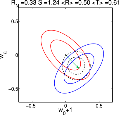
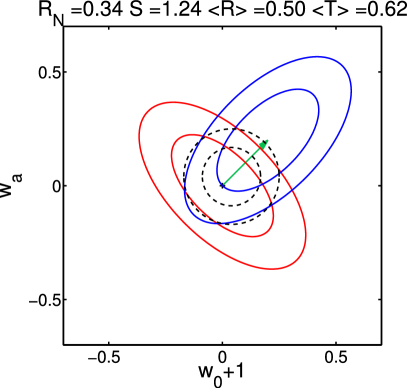
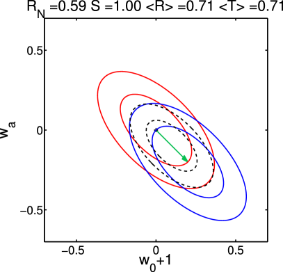
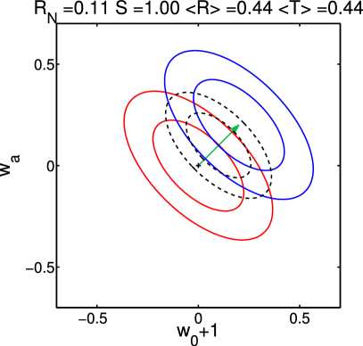
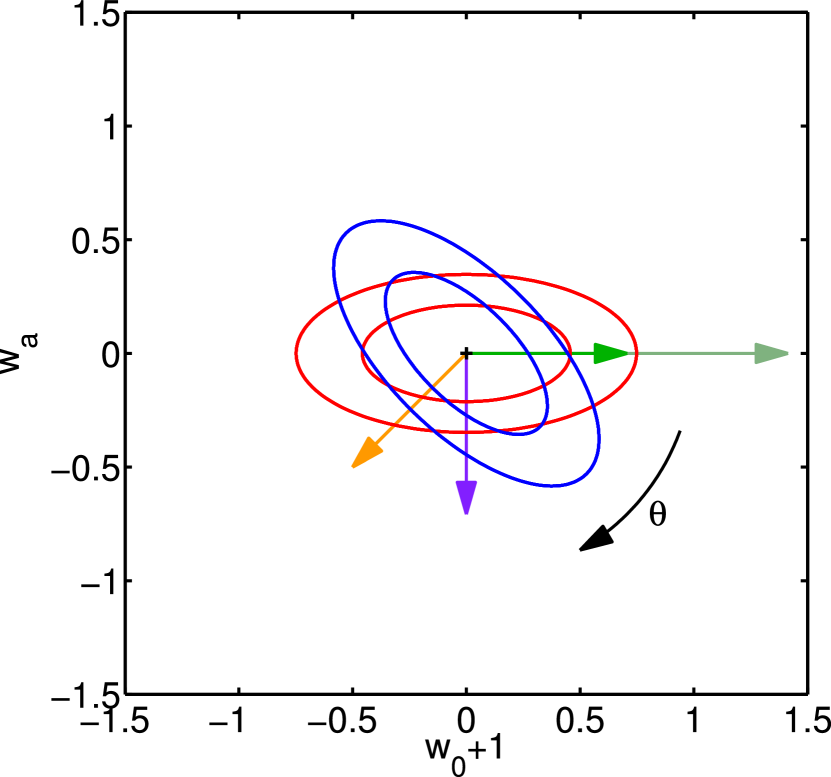
Armed with the above intuition, we now consider in Fig. 1, a numerical illustration of 4 different cases for the relative orientation of the two probes (orthogonal or parallel) and the direction of the bias vector (along the short or long semiaxis). The two sets of iso-likelihood contours enclose 68% and 95% confidence levels; as above, the second probe (blue contours) has the same area as the first (i.e., $L_{1}=L_{2}$), but its degeneracy direction can be rotated, and its maximum likelihood value is displaced from the true value by a systematic bias (of fixed length in all cases), given by the green vector. The first probe (red contours) is assumed to be unbiased. The prior is $\Pi=\text{diag}(1,1)$ (i.e. a prior of 1.0 in each parameter with no correlations imposed). For each case, we give the corresponding statistical FoM, Eq. (12), the robustness FoMs, (27) and (29), and the total FoM (for the averaged robustness), Eq. (34).

The robustness FoM (with or without averaging) depends both on the direction along which the bias is directed and on the relative orientation of the degeneracy directions of the two probes. When the bias is directed along the degeneracy direction of probe 1 and probe 2 is aligned along that direction (lower left panel), the robustness is maximal. It decreases if the two probes are orthogonal to each other, since this reduces the degree of overlap between them (upper panels). Finally, robustness is smallest when the two probes are aligned but the bias is direct orthogonally w.r.t the degeneracy direction (lower right panel), as argued above. Looking ahead to the application of the robustness formalism to the dark energy equation of state parameters in the next section, we can anticipate here that the most relevant case is the one where the two probes are similarly oriented (bottom panels of Fig. 1). This is because different dark energy probes are typically degenerate in the equation of state parameters along quite similar directions. Therefore, their relative robustness can be expected to depend mainly on the orientation of the bias w.r.t. the main degeneracy direction.

The statistical FoM is largest when the probes are orthogonal to each other, as expected. Notice that the statistical FoM is unaffected by the bias, and only depends on the relative alignment of the two probes. For a given orientation and size of the bias vector, the total FoM allows one to decide which configuration for probe 2 is to be preferred. For the example of Fig. 1, if the bias vector points along the degeneracy direction of probe 1 (left-hand side panels), one would prefer probe 2 to be aligned with probe 1 ($\langle T\rangle=0.71$) as opposed to probe 2 being orthogonal to probe 1 ($\langle T\rangle=0.61$). If instead the bias is orthogonal to the degeneracy of probe 1 (right-hand side panels), then the best choice for probe 2 is for it to be orthogonal to probe 1 ($\langle T\rangle=0.62$ compared to $\langle T\rangle=0.44$).

Figure 1: Illustration of statistical and robustness FoM for a future probe (blue ellipses, 68% and 95% C.L.) which is systematically biased w.r.t. the present-day constraints (red ellipses) in the direction given by the green bias vector. The black dotted ellipses represent the combined constraints. Notice that the statistical FoM (S) does not change in the presence of a systematic bias.

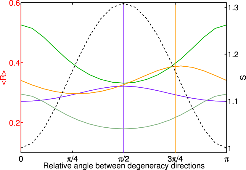
We can also ask what is the optimal orientation of probe 2 with respect to probe 1 if one wanted to maximise its robustness, given a bias direction. In Fig. 2, we plot both the statistical and the average robustness FoMs as a function of the rotation angle between the principal direction of the two probes. The average robustness is evaluated for 3 different directions of the bias (coloured vectors in the top panel). We notice once more that the statistical FoM is maximised when the probes are orthogonal. However, the robustness FoM is maximised when the degeneracy direction of probe 2 is close to being aligned with the direction of the bias vector, as this maximizes the overlap with probe 1 even when probe 2 suffers from a systematic error. Finally, increasing the length of the bias by a factor of 2 (fainter green vector in the top panel) reduces the overall average robustness.

In summary, the robustness of a future probe is a function of its statistical properties (i.e., the direction along which its main degeneracy is aligned, compared with the degeneracy direction of probe 1) as well as of the direction and size of the systematic bias. The performance of a future probe should be assessed by considering simultaneously its statistical power but also its robustness to systematics. Optimizing a future dark energy experiment in terms of its statistical errors alone would generically lead to an experiment which is less robust, for a given overall level of plausible systematics. Any optimization procedure should therefore involve the complementary criteria of statistical strenght and robustness to systematic bias.

Figure 2: Dependency of FoMs on the angle between the degeneracy direction of the two probes. Upper panel: the red (blue) ellipses represent the 68% and 95% likelihood contours of probe 1 (probe 2, which is potentially biased). The degeneracy direction of probe 2 is offset by an angle $\theta$ w.r.t probe 1. The three vectors gives three possible directions for the bias. Lower panel: value of statistical FoM $S$ (black dashed line, right-hand axis), and average robustness FoM, $\langle R\rangle$, (coloured solid lines, left-hand axis, colour and thickness matching the bias vectors in the upper panel), as a function of the relative angle $\theta$. Vertical coloured lines give the angle of each bias vector.

We now turn to applying the above concept to the concrete scenario of two classes of future dark energy missions, namely type Ia SN and BAO measurements.

4 Robustness of Future Dark Energy Probes

We consider a simple and widely used phenomenological description of an evolving dark energy model, where the equation of state is $w(z)=w_{0}+w_{a}z/(1+z)$, characterized by the two free parameters $(w_{0},w_{a})$ (Chevallier & Polarski, 2001; Linder, 2003). For probe 1 (representing current constraints on $w_{0},w_{a}$) we take a Gaussian approximation to the joint likelihood resulting from the combination of Union 2 SNe Ia data (Amanullah et al., 2010), SDSS BAO (Percival et al., 2010), WMAP7 measurements of the shift parameters (Komatsu et al., 2010), and SHOES measurements of the Hubble constant (Riess et al., 2009). We further assume a flat Universe. For the prior on the dark energy parameters, we take a Gaussian centered at $(w_{0}+1,w_{a})=(0,0)$ with Fisher matrix $\Pi=\text{diag}(1,1/100)$. In the following, when we look at the Fisher matrix we mean the 2D marginalised Fisher matrix (i.e., marginalised down to the dark energy parameter space). Although in the rest of this paper we focus exclusively on the robustness FoM for dark energy parameters, we note that our robustness formalism is equally applicable to any other cosmological parameter one is interested in.

In order to evaluate robustness, we need to specify the bias vector $b$. There are several plausible ways of doing this, and the outcome will depend on what one thinks a possible systematic bias might be due to. In our case, in order to illustrate our new FoM, we determine $b$ by assuming a possible systematic bias in the probe’s observables, and then projecting the resulting systematic shift onto the dark energy parameter space of interest, as described in detail below. We stress that this is by no means the only procedure by which one can estimate $b$. Other assumptions about the origin of systematic errors will in general lead to a different $b$, and therefore to a different value for the robustness of the future probe.

4.1 Future SN Ia Measurements

We consider a survey dedicated to observing type Ia supernovae from space, with a redshift distribution like the one expected from SNAP, with 2000 SNe distributed as in Kim et al. (2004), plus a low-$z$ sample of 300 SNe distributed uniformly in the redshift range $0.03<z<0.08$. The projected SNAP magnitude errors include both statistical and systematic components, and are modelled as follows:

$$\sigma_{b}^{2}=\left[\frac{0.15^{2}}{N_{b}}+A_{\text{syst}}^{2}\left(\frac{1+z_{b}}{1+z_{\text{max}}}\right)^{2}\right],$$ (43)

where $N_{b}$ is the number of SNe in each bin centered at $z_{b}$ and of width $dz=0.1$. The second term on the right-hand side of Eq. (43) models a systematic floor that increases linearly with $z$ up to a maximum of $A_{\text{syst}}$ mag per $dz=0.1$ bin at $z_{{\rm max}}=1.7$ (Linder & Huterer, 2003). In order to evaluate the robustness of SNa data for different levels of systematics, we will consider values of $A_{\text{syst}}=0.01,0.02,0.05$.

We assume a flat universe with four parameters relevant for this analysis, matter density relative to critical $\Omega_{M}$, equation of state today $w_{0}$, its variation with scale factor $w_{a}$, and a nuisance offset in the Hubble diagram $\mathcal{M}$. Marginalizing over $\Omega_{M}$ and $\mathcal{M}$ and assuming $A_{\text{syst}}=0.02$, we find that our fiducial survey produces statistical errors of $\sigma_{w_{0}}=0.075$ and $\sigma_{w_{a}}=0.30$, corresponding to the black 68% C.L. ellipse in Fig. 3.

The bias in the dark energy parameters, $b$, reconstructed from SN measurements induced by an arbitrary bias in the observed magnitudes $\delta m(z)$ can be derived from the Fisher matrix for SNe (e.g. Knox et al. (1998); Huterer & Turner (2001)), and is given by

$$b_{i} = \sum_{j}(F^{-1})_{ij}\sum_{\alpha}\frac{dm(z_{\alpha})}{d\mu_{j}}\,\frac{1}{\sigma_{\alpha}^{2}}\,\delta m_{{\rm sys}}(z_{\alpha})$$ (44)

$$\equiv \sum_{\alpha}c_{\alpha}^{(i)}\,\delta m_{{\rm sys}}(z_{\alpha})$$ (45)

where $\mu_{i}$ are the cosmological parameters, $c_{\alpha}^{(i)}\equiv\sum_{j}(F^{-1})_{ij}(dm(z_{\alpha})/d\mu_{j})/\sigma_{\alpha}^{2}$ and where $\alpha$ runs over redshift bins. We adopt a systematic bias of the same form as the “floor” that was previously included in the total statistical error:

$$\delta m_{{\rm sys}}(z_{\alpha})=A_{\text{syst}}\left(\frac{1+z_{\alpha}}{1+z_{\text{max}}}\right)$$ (46)

Bias of this magnitude leads to the bias on cosmological parameters which can be calculated using Eqs. (45) and (46), and is shown as the blue curve in Fig. 3. Each point on the curve shows cumulative contributions to the excursion in $w_{0}$ and $w_{a}$ around the fiducial model (with $(w_{0},w_{a})=(-1,0)$) for each of the 16 redshift bins we consider, $z\in[0.1,0.2],\ldots,z\in[1.6,1.7]$. In other words, points on the blue curve show cumulative contribution of the sum in Eq. (45).

Figure 3: Systematic bias in the $w_{0}$-$w_{a}$ plane for future SNIa data. The square denotes our fiducial value and the ellipse gives the 68% CL statistical contour from future SNIa data. The blue curve shows the systematic bias given by Eq. (46), with points showing cumulative contributions from each of the 16 redshift bins – that is, cumulative value of the sum in Eq. (45).For clarity, we explicitly label bias contributions accumulated by redshifts $z=1$ and $z=1.7$. The red segments denote the worst-case bias, where the sign of $\delta m(z)$ at each redshift bin conspires to shift the $(w_{0},w_{a})$ value away from the true value (“Maximum excursion bias”); see Eq. (47). For clarity, we have also plotted the biases with the opposite sign relative to the fiducial model parameter values.

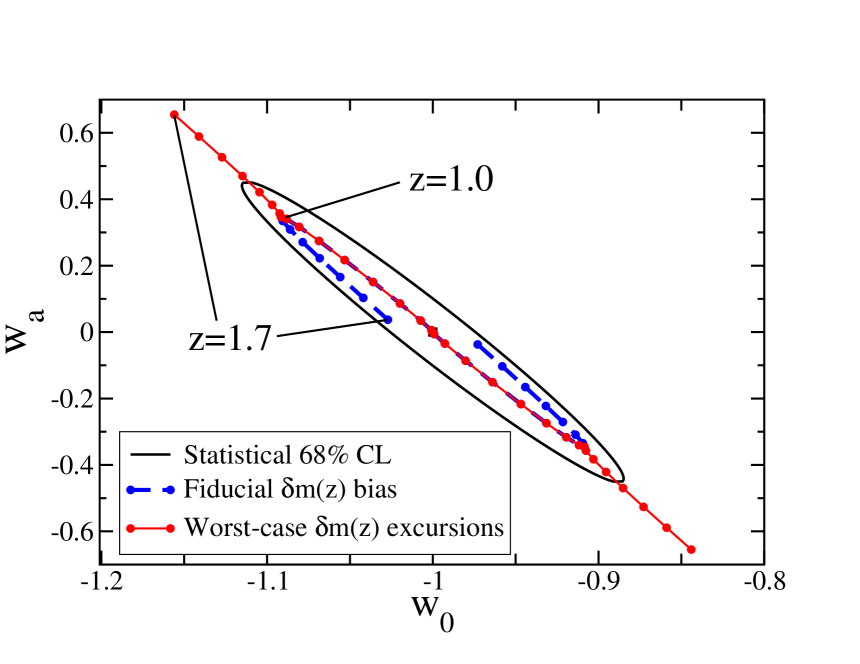
But this form of the bias assumes that the excursions in $\delta m(z_{\alpha})$ are of the same sign (taken to be positive), and equal to the maximum allowed value in Eq. (46). The worst-case bias to the dark energy parameters is obtained if $\delta m(z_{\alpha})$ changes sign in each redshift bin just so as to maximize the excursion in $w_{0}$ and $w_{a}$. Such a worst-case bias can be straightforwardly calculated (Huterer & Takada, 2005)

$$b_{i}^{{\rm worst}}=\sum_{\alpha}|c_{\alpha}^{(i)}|\,\delta m_{{\rm sys}}(z_{\alpha})$$ (47)

for a single dark energy parameter $\mu_{i}$, where $\delta m_{{\rm sys}}(z_{\alpha})>0$ was taken by default. In other words, the systematic error takes a plus or minus sign equal to that of the coefficient $c_{\alpha}^{(i)}$ in each redshift bin . Such a worst-case excursion in the $(w_{0},w_{a})$ plane is shown as the red curve with points in Fig. 3. We call this scenario the “maximum excursion bias” (MEB), and use it as an estimate for the bias vector $b$ in the computation of our robustness FoM.

4.2 Future Baryonic Acoustic Oscillations Measurements

The second class of future probe we consider consists of a full-sky spectroscopic redshift survey modelling a future spacee mission with specifications close to WFIRST or Euclid (or a Stage-IV mission in the language of the DETF). The probe is fully specified by choosing a number of redshift bins and giving the expected number densities of galaxies per bin and the sky coverage, assumed here to be 20,000 square degrees. Table 1 gives the redshift binning and the galaxy number densities, taken from the data published by the Euclid collaboration (Laureijs et al., 2009). We assume however that only half of these galaxies can be effectively employed (efficiency $\epsilon=0.5$), corresponding to one half of values in the Table.

$z$	$n(z)\times 10^{-3}$
0.5-0.7	$3.56$
0.7-0.9	$2.42$
0.9-1.1	$1.81$
1.1-1.3	$1.44$
1.3-1.5	$0.99$
1.5-1.7	$0.55$
1.7-1.9	$0.29$
1.9-2.1	$0.15$

Table 1: Expected galaxy number densities per redshift bin in units of ($h/$Mpc)³ for the Euclid survey.

In order to forecast the statistical errors on dark energy parameters, we adopt the Fisher matrix method of Seo & Eisenstein (2003, 2007), also employed in Amendola et al. (2005). Here we give a short summary of the method and refer to these papers for the implementation details. In the limit where the survey volume $V_{\rm survey}$ is much larger than the scale of any features in $P_{\rm obs}(k)$, it has been shown that the redshift survey Fisher matrix in a redshift bin $\Delta z$ can be approximated as (Tegmark, 1997)

$$F_{ij} = \int_{-1}^{1}\int_{k_{\rm min}}^{k_{\rm max}}\frac{\partial\ln P_{\rm obs}(k,\mu)}{\partial\mu_{i}}\frac{\partial\ln P_{\rm obs}(k,\mu)}{\partial\mu_{j}}$$ (48)

$$\times V_{\rm eff}(k,\mu)\frac{2\pi k^{2}dkd\mu}{2(2\pi)^{3}}$$

Here, $k,\mu$ are the wavevector moduls and direction cosine with respect to the line of sight, respectively, and the derivatives are evaluated on the parameters $\mu_{i}$ of the fiducial model. The upper cut-off $k_{\rm max}$ is chosen so as to avoid the non-linear regime, while the large-scale cut-off $k_{\rm min}$ is set to $0.001h$/Mpc but its precise value has a very weak impact. $V_{\rm eff}$ is the effective volume of the survey:

$$V_{\rm eff}(k,\mu)=\left[\frac{{n_{\rm g}}P_{\rm g}(k,\mu)}{{n_{\rm g}}P_{\rm g}(k,\mu)+1}\right]^{2}V_{\rm survey},$$ (49)

where $V_{\rm survey}$ is the 20,000 square degrees survey volume contained in a given redshift bin. The galaxy comoving number density $n_{\rm g}(z)$ is assumed to be spatially constant within a redshift bin, while $P_{g}$ is the galaxy spectrum defined below. The total Fisher matrix is obtained by summing over all the redshift bins of Table 1. The matter power spectrum in any given cosmology can be written in terms of the spectrum in the fiducial (or “reference”, subscript “ref”) cosmology as

$$P_{\rm obs}(k_{{\rm ref}\perp},k_{{\rm ref}\parallel},z)=\frac{D(z)_{\rm ref}^{2}H(z)}{D(z)^{2}H(z)_{\rm ref}}P_{\rm g}(k_{{\rm ref}\perp},k_{{\rm ref}\parallel},z)+P_{\rm shot}\,,$$ (50)

where

$$P_{\rm g}(k_{{\rm ref}\perp},k_{{\rm ref}\parallel},z)=b(z)^{2}\left[1+\beta(z)\frac{k_{{\rm ref}\parallel}^{2}}{k_{{\rm ref}\perp}^{2}+k_{{\rm ref}\parallel}^{2}}\right]^{2}P_{{\rm matter}}(k,z)\,.$$ (51)

In Eq. (50), $H(z)$ and $D(z)$ are the Hubble parameter and the angular diameter distance, respectively, and the prefactor encapsulates the geometrical distortions due to the Alcock-Paczynski effect (Seo & Eisenstein, 2003, 2007). $k_{\perp}$ and $k_{\parallel}$ are the wave-numbers across and along the line of sight in the given cosmology, and they are related to the wave-numbers calculated assuming the reference cosmology by $k_{{\rm ref}\perp}=k_{\perp}D(z)/D(z)_{\rm ref}$ and $k_{{\rm ref}\parallel}=k_{\parallel}H(z)_{\rm ref}/H(z)$. $P_{\rm shot}$ is the unknown white shot noise that remains even after the conventional shot noise of inverse number density has been subtracted (Seo & Eisenstein, 2003, 2007). In Eq. (51), $b(z)$ is the linear bias factor between galaxy and matter density distributions, $f_{g}(z)$ is the linear growth rate, $\beta(z)=f_{g}(z)/b(z)$ is the linear redshift-space distortion parameter (Kaiser, 1987) and $P_{{\rm matter}}$ is the linear matter power spectrum. The fiducial values for the bias and the growth factor are $b(z)=1$ and $f_{g}=\Omega_{M}^{0.545}$, respectively. In di Porto et al. (2011) it has been shown that the precise fiducial value of $b(z)$ does not have a large impact on the results.

This method employs all the information contained in the power spectrum, including the redshift distortion, not just the position of the baryonic wiggles. As above, we choose a flat fiducial cosmology with $\Omega_{M}=0.24$, $h=0.7$, $\Omega_{DE}=0.737$, $\Omega_{K}=0$, $\Omega_{b}h^{2}=0.0223$, $n_{s}=0.96,$ $w_{0}=-1,w_{a}=0$. Unlike in the SN case, we do not impose an explicit systematic floor in the forecasted BAO errors; the finite sky coverage and density of galaxies provide an effective floor for any given BAO survey. As mentioned above, beside the cosmological parameters, for each redshift bin we also include as free parameters to be differentiated (and then marginalized) in the Fisher matrix a matter-galaxy bias factor and an additive shot noise term in the power spectrum (for details see Amendola et al. (2005)). These terms act as additional effective systematic floors.

The systematic effect we assume for the redshift survey is a fractional error in estimating the value of the Hubble function $H(z_{i})$ of magnitude $A_{\text{syst}}=0.001,0.002,0.005$ in each bin $i$. Such a bias in $H(z)$ propagates to a bias in the angular diameter distance $D(z)$, as well, if the standard flat-space Friedman-Robertson-Walker relation

$$D(z)=(1+z)^{-1}\int_{0}^{z}\frac{dz^{\prime}}{H(z^{\prime})}$$ (52)

holds true, which we assume here. The angular diameter distance bias is then related to the Hubble function bias by

$$\delta(\ln D)=-\delta(\ln H)\frac{H(z)}{(1+z)D(z)}\int_{0}^{z}\frac{dz^{\prime}}{H^{2}(z^{\prime})}.$$ (53)

where we have used the assumption that the bias in $\ln H$ is redshift-independent. This simple choice for modelling systematic errors in BAO is meant to approximately capture a possible systematic shift in the baryon peak position due to e.g. the presence of isocurvature modes (Zunckel et al., 2010) or non-linear effects, of the kind described e.g. in Seo et al. (2008). A more realistic choice of systematic errors is difficult to model accurately (as, for example, a bias in $H(z)$ and/or $D(z)$ also modifies in general the whole spectrum behavior and the redshift distortions), and it is left for future work. Our present choice is meant as a simple illustration of the method and a first step towards evaluating the robustness FoM.

If instead of the true matter power spectrum, $P(k)$, we measure a spectrum that contains a systematic error $\delta s_{\alpha}=\delta(\ln H_{\alpha})$ or $\delta s_{\alpha}=\delta(\ln D_{\alpha})$ in the value of $H(z_{\alpha})$ and $D(z_{\alpha})$ (where the systematic shifts are related by Eq. (53)), the maximum likelihood estimate for the $i$-th parameter will be shifted w.r.t. its true value by a bias given by (see e.g. Taylor et al. (2007))

$$\delta\mu_{i} = F_{ij}^{-1}\left[\frac{1}{8\pi^{2}}\int d\mu k^{2}dk\frac{\partial\ln P}{\partial\mu_{j}}\frac{\partial\ln P}{\partial s_{\alpha}}\right]\delta s_{\alpha}$$ (54)

$$\equiv c^{(i)}_{\alpha}\delta s_{\alpha}$$

(sum over repeated indexes). Analogously to the previous subsection we have defined

$$c^{(i)}_{\alpha}\equiv F_{ij}^{-1}\left[\frac{1}{8\pi^{2}}\int d\mu k^{2}dk\frac{\partial\ln P}{\partial\mu_{j}}\frac{\partial\ln P}{\partial s_{\alpha}}\right]\,.$$ (55)

In this particular case, however, the $i$-th parameters coincide with $\delta s_{i}=\delta(\ln H_{i}),\delta(\ln D_{i})$ and therefore the matrix $c^{(i)}_{\alpha}$ is the identity matrix. We can then directly project the systematic bias onto the dark energy parameters $(w_{0},w_{a})$, obtaining a bias vector $b$ of the form

$$\begin{split}b_{l}&=\sum_{\beta}\left(\frac{\partial w_{l}}{\partial\ln H(z_{\beta})}\right.-\\ &\frac{H(z_{\beta})}{(1+z_{\beta})D(z_{\beta})}\left.\int_{0}^{z_{\beta}}\frac{dz^{\prime}}{H^{2}}\frac{\partial w_{l}}{\partial\ln D(z_{\beta})}\right)\,\delta\ln H(z_{\beta})\end{split}$$ (56)

where $\delta\ln H(z_{\beta})=0.001,0.002,0.005$, the subscript $\beta$ runs over the redshift bins, and $l=0,a$. We have chosen to consider systematic shifts in the range of 0.1% to 0.5% to reflect ballpark estimates of what BAO systematic errors due e.g. to residual non-linear corrections might be. We stress once more that this is a simplified treatment used here mainly for illustration purposes of our method.

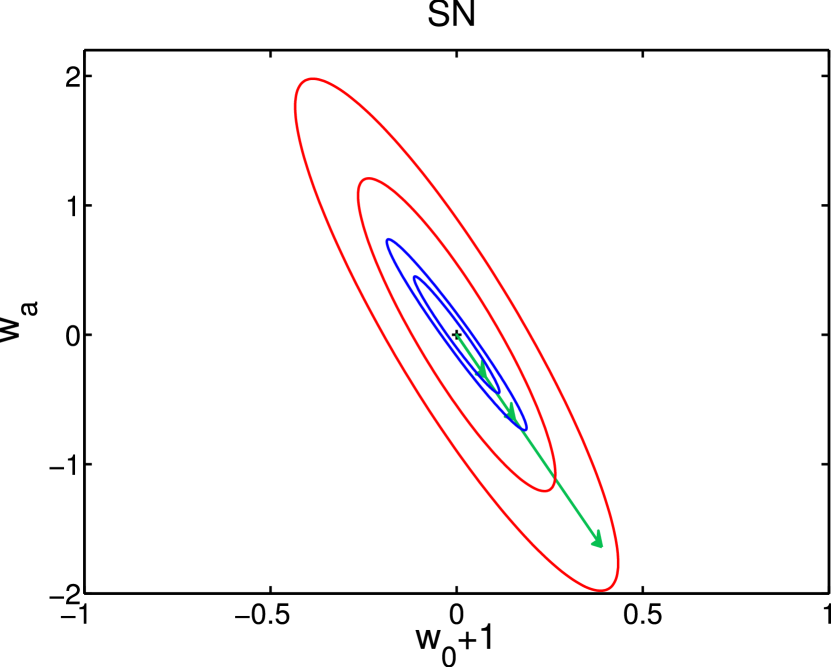
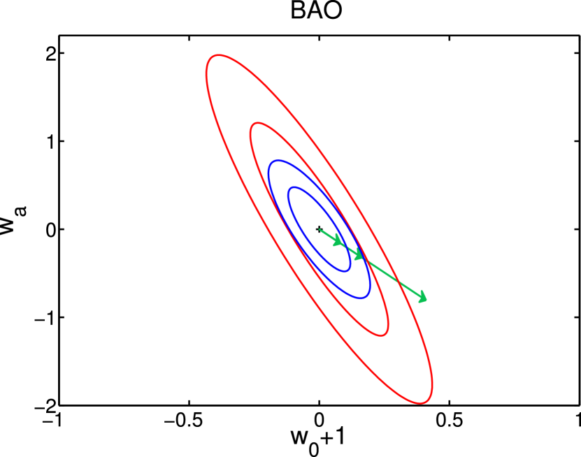
We evaluate $b_{l}$ for each redshift bin and then estimate the maximum bias by following the same method discussed in the previous subsection. Here it happens that the contributions to $b_{l}$ are always positive and therefore automatically select the worst case scenario, i.e., the maximum excursion bias. The resulting maximum excursion bias for different levels of systematics is shown as the green vectors in the bottom panel of Fig. 4, together with the statistical errors from our BAO probe (blue ellipses) and current constraints (red ellipses), plotted for comparison.

5 Results

Our results for the statistical and robustness FoMs are summarized in Table 2, where we give the values of our robustness, statistical and total FoM. We also show the value of the DETF FoM (normalized to the value obtained from the current probes) for comparison.

First, by inspecting Fig. 4, we notice that the systematic bias projected onto the $(w_{0},w_{a})$ plane is much better aligned with the degeneracy direction of the probes for SNIa than for BAO. From our discussion in section 3, this leads to expect a higher value for the robustness FoM for SNIa than for BAO. Also, the size of the bias vectors in the dark energy parameters is roughly comparable for SNIa and BAO, although in the latter case we have adopted a bias in the observables ($H$ and $D$) which is a factor of 10 smaller than for the SNIa observables (the magnitudes). Table 2 shows that indeed both the robustness and the average robustness FoMs are slightly larger for SNIa than for BAO across the range of systematic error levels we adopted for each probe. This is a consequence of the fact that the BAO bias leads to a smaller degree of overlap of the BAO constraints with the present-day constraints, which is a more serious lack of robustness than for the SNIa. In the latter case, although the bias vectors are slightly larger in the dark energy parameters (typically by a factor of 2, cf Table 2), the bias direction is well aligned with the statistical degeneracy, and therefore the reduction in the overlap between the present constraints and future SNIa constraints is less severe, translating in a higher robustness. For the highest level of systematic error in each case (0.5% for BAO and 5% for SNIa), we find that the robustness FoM for BAO is about a factor of 10 smaller than for SNIa. The average robustness of BAO is also smaller, but only by about 1/3, which reflects the more balanced assessment given by the average robustness. Thus, for our particular choice of systematics, our findings run against the general lore that BAO observations are more robust to systematics than SNIa.

In terms of our statistical FoM, the SNIa survey is better by a factor of about 3, in good agreement with the result obtained from the usual DETF FoM. Taken together, the better values of both the statistical and robustness FoM for SNIa lead to a higher value of the total FoM for SNIa than for BAO.

It is important to stress that our robustness results above are not a generic feature of SNIa and BAO observations. Rather, they reflect our specific choices for the systematic bias in the observables for BAO and SNIa. Other choices of systematic bias are possible and will in general give a different results for the robustness, which we shall explore in a dedicated paper.

Figure 4: Construction of the robustness FoM for a future SNIa survey (top panel) and a future BAO Euclid-like survey (bottom panel). Red ellipses show current 68%, 95% constraints (in a Gaussian approximation) from a combination of all available probes, blue ellipses show projected constraints from the future probe at the fiducial point (assumed to be $\Lambda$CDM). The green vectors show the systematic maximum excursion bias (MEB) for systematic erros of 1%, 2% and 5% for SNIa and 0.1%, 0.2% and 0.5% for BAO.

			BAO			SNIa
			Maximum excursion bias			Maximum excursion bias
Fom	Symbol	Defined in	0.1%	0.2%	0.5%	1%	2%	5%
Robustness	$R_{N}$	Eq. (27)	$1.4$	$0.83$	$0.026$	$1.7$	$1.3$	$0.24$
Average robustness	$\langle R\rangle$	Eq. (32)	1.4	1.1	0.54	1.7	1.4	0.81
Statistical FoM	$S$	Eq. (12)	2.7			7.0
Total FoM	$T_{N}$	Eq. (33)	3.6	$2.2$	$0.070$	11.9	9.1	1.7
Total average FoM	$\langle T\rangle$	Eq. (34)	3.8	2.9	1.4	11.9	9.8	5.7
Bias length	$|b|$	caption	0.18	0.36	0.90	0.34	0.68	1.7
DETF FoM		Eq. (9)	4.4			13

Table 2: Robustness and statistical Figure of Merits for future BAO and SNIa surveys, for different levels of systematic errors in the observables. We also give the DETF FoM for comparison (normalized to its value from current constraints). We also give the length of the bias vector $b$ in the $(w_{0},w_{a})$ plane. The Maximum excursion bias errors refer to both $D(z_{b})$ and $H(z_{b})$ in the case of BAO, and $m(z_{b})$ in the case of SNIa.

6 Conclusions

We have introduced a new formalism to quantify the robustness of future dark energy probes to systematic bias, and argued that this important new quantity should be taken into account when evaluating the performance of future surveys. In constrast to usual measures of statistical performance, our robustness FoMs depend on the direction and size of the systematic bias induced in the dark energy parameters by residual systematics in the observables. We have thus described an approach to include the effect of systematic errors in the dark energy figures of merit.

We have applied this formalism to future SNIa and BAO probes by developping a simple phenomenological model of possible residual systematic errors. Our results indicate that – for the specific choice of systematics adopted here – SNIa are slightly more robust to systematics than BAO, despite having assumed a systematic shift in the observables for SNIa which is a factor of 10 larger than for BAO. Coupled with the higher statistical performance of SNIa, this would lead to prefer SNIa over BAO in terms of their overall FoM. It is clear however that this particular result cannot be generalized beyond our choice of systematics and surveys. In a future work we will investigate how this result change by adopting more refined descriptions of the systematic bias for each probe.

Acknowledgements. L.A., D.H. and R.T. would like to thank the Galileo Galilei Institute for Theoretical Physics for hospitality. M.C.M. would like to thank the University of Heidelberg for hospitality. L.A. would like to thank Imperial College London for hospitality. R.T. would like to thank the INFN and the EU FP6 Marie Curie Research and Training Network “UniverseNet” (MRTN-CT-2006-035863) for partial support. L.A. is partially supported by DFG TRR33 “The Dark Universe”. DH is supported by DOE OJI grant under contract DE-FG02-95ER40899, NSF under contract AST-0807564, and NASA under contract NNX09AC89G.

Appendix A

The generalization of Eq. (20) to an arbitrary number of probes proceeds as follows. First, we notice that one can always summarize current constraints from several observations in one single joint posterior. Let us call the data from the combination of all available present-day probes $d_{0}$ (with Fisher matrix $F_{0}$). If one wishes to consider $N$ future probes, we can ask whether all of the $N$ probes are mutually compatible. Eq. (15) gives in this case

$$R_{\text{all}} = \frac{p(d_{N}d_{N-1}\dots d_{1}|d_{0})}{\prod_{j=1}^{N}p(d_{j}|d_{0})}$$ (58)

$$= \prod_{j=1}^{N}\frac{p(d_{j}|d_{j-1}\dots d_{1}d_{0})}{p(d_{j}|d_{0})}$$ (59)

$$= \prod_{j=2}^{N}\frac{p(d_{j}|d_{j-1}\dots d_{1}d_{0})}{p(d_{j}|d_{0})}$$ (60)

where in the last line we have cancelled out the very last term in both the numerator and the denominator, so that the sum starts with $j=2$. We now refer to Eq. (17) to obtain

$$p(d_{j}|d_{j-1}\dots d_{1}d_{0})=\mathcal{L}_{0}^{(j)}\frac{|F_{012\dots(j-1)}|^{1/2}}{|F_{012\dots j}|^{1/2}}$$

$$\times \exp\left[-\frac{1}{2}\left(\mu_{j}^{t}L_{j}\mu_{j}\right.\right.$$

$$+ \mu_{012\dots(j-1)}^{t}F_{012\dots(j-1)}\mu_{012\dots(j-1)}$$

$$- \left.\left.\mu_{012\dots j}^{t}F_{012\dots j}\mu_{012\dots j}\right)\right],$$

where the definitions correspond to those before, so that $F_{012\dots j}\equiv F_{0}+\sum_{i=1}^{j}L_{i}$, and in particular $F_{012\dots N}\equiv F$. Notice already that most terms in the numerator of Eq. (60) will cancel. Similarly, following Eq. (18)

$$p(d_{j}|d_{0}) = \mathcal{L}_{0}^{(2)}\frac{|F_{0}|^{1/2}}{|F_{0j}|^{1/2}}$$

$$\times \exp\left[-\frac{1}{2}\left(\mu_{j}^{t}L_{j}\mu_{j}+\mu_{0}^{t}F_{0}\mu_{0}-\mu_{0j}^{t}F_{0j}\mu_{0j}\right)\right],$$

Now one can evaluate Eq. (60) with the help of Eqs. (Appendix A) and (Appendix A):

$$\begin{split}R_{\text{all}}&=\frac{|F_{01}|^{1/2}}{|F|^{1/2}}\prod_{j=2}^{N}\frac{|F_{0}|^{-1/2}}{|F_{0j}|^{-1/2}}\times\exp\left[-\frac{1}{2}(\mu_{01}^{t}F_{01}\mu_{01}-\mu^{t}F\mu\right.\\ &-\left.(N-1)\mu_{0}^{t}F_{0}\mu_{0}+\sum_{j=2}^{N}\mu_{0j}^{t}F_{0j}\mu_{0j})\right]\end{split}$$ (63)

We thus obtain for the robustness

$$\begin{split}\ln R_{\text{all}}&=\frac{1}{2}\left(\sum_{i=1}^{N}\ln|F_{0i}|-(N-1)\ln|F_{0}|-\ln F\right)\\ &-\frac{1}{2}(\sum_{i=1}^{N}\overline{\mu}_{0i}^{t}F_{0i}\overline{\mu}_{0i}-(N-1)\mu_{0}^{t}F_{0}\mu_{0}-\mu^{t}F\mu),\end{split}$$ (64)

which generalizes Eq. (20).

References

- Albrecht et al. (2006) Albrecht A., et al., 2006, astro-ph/0609591
- Albrecht et al. (2009) Albrecht A., et al., 2009, arXiv:0901.0721
- Albrecht & Bernstein (2007) Albrecht A. J., Bernstein G., 2007, Phys. Rev., D75, 103003
- Amanullah et al. (2010) Amanullah et al., 2010, Ap.J., 716, 712
- Amendola et al. (2005) Amendola L., Quercellini C., Giallongo E., 2005, Mon. Not. R. Astron. Soc., 357, 429
- Chevallier & Polarski (2001) Chevallier M., Polarski D., 2001, International Journal of Modern Physics D, 10, 213
- Crittenden et al. (2009) Crittenden R. G., Pogosian L., Zhao G.-B., 2009, JCAP, 0912, 025
- Feroz et al. (2008) Feroz F., et al., 2008, JHEP, 10, 064
- Feroz et al. (2009) Feroz F., Hobson M. P., Roszkowski L., Ruiz de Austri R., Trotta R., 2009
- Hobson et al. (2002) Hobson M. P., Bridle S. L., Lahav O., 2002, Mon. Not. Roy. Astron. Soc., 335, 377
- Huterer & Takada (2005) Huterer D., Takada M., 2005, Astropart. Phys., 23, 369
- Huterer & Turner (2001) Huterer D., Turner M. S., 2001, Phys. Rev., D64, 123527
- Kim et al. (2004) Kim A. G., Linder E. V., Miquel R., Mostek N., 2004, Mon. Not. R. Astron. Soc., 347, 909
- Knox et al. (1998) Knox L., Scoccimarro R., Dodelson S., 1998, Phys. Rev. Lett., 81, 2004
- Komatsu et al. (2010) Komatsu et al., 2010, arXiv:1001.4538
- Laureijs et al. (2009) Laureijs R., et al., 2009, arXiv:0912.0914
- Linder (2003) Linder E. V., 2003, Phys. Rev. Lett., 90, 091301
- Linder & Huterer (2003) Linder E. V., Huterer D., 2003, Phys. Rev., D67, 081303
- Mortonson et al. (2010) Mortonson M. J., Huterer D., Hu W., 2010, Phys. Rev., D82, 063004
- Percival et al. (2010) Percival W. J., et al., 2010, Mon. Not. R. Astron. Soc., 401, 2148
- Riess et al. (2009) Riess A. G., Macri L., Casertano S., Sosey M., Lampeitl H., Ferguson H. C., Filippenko A. V., Jha S. W., Li W., Chornock R., Sarkar D., 2009, The Astrophysical Journal, 699, 539
- Seo & Eisenstein (2003) Seo H., Eisenstein D. J., 2003, Ap.J., 598, 720
- Seo & Eisenstein (2007) Seo H., Eisenstein D. J., 2007, Ap.J., 665, 14
- Seo et al. (2008) Seo H., Siegel E. R., Eisenstein D. J., White M., 2008, Ap. J., 686, 13
- Taylor et al. (2007) Taylor A. N., Kitching T. D., Bacon D. J., Heavens A. F., 2007, Mon. Not. R. Astron. Soc., 374, 1377
- Trotta et al. (2010) Trotta R., Kunz M., Liddle A. R., 2010, arXiv:1012.3195
- Trotta (2008) Trotta R., 2008, Contemp. Phys., 49, 71
- Wang (2008) Wang Y., 2008, Phys. Rev., D77, 123525
- Zunckel et al. (2010) Zunckel C., Okouma P., Kasanda S. M., Moodley K., Bassett B. A., 2010, arXiv:1006.4687
- Tegmark (1997) Tegmark M., 1997, Phys. Rev. Lett. 79, 3806
- Kaiser (1987) Kaiser N., 1987, Mon. Not. R. Astron. Soc., 227, 1
- di Porto et al. (2011) di Porto C., Amendola L., Branchini E., 2011, arXiv:1101.2453