A coherent triggered search for single spin compact binary coalescences in gravitational wave data

Abstract

In this paper we present a method for conducting a coherent search for single spin compact binary coalescences in gravitational wave data and compare this search to the existing coincidence method for single spin searches. We propose a method to characterize the regions of the parameter space where the single spin search, both coincident and coherent, will increase detection efficiency over the existing non-precessing search. We also show example results of the coherent search on a stretch of data from LIGO’s fourth science run but note that a set of signal based vetoes will be needed before this search can be run to try to make detections.

1 Introduction

The Laser Interferometer Gravitational-wave Observatory (LIGO) and Virgo scientific collaborations have performed many searches for compact binary coalescence (CBC) signals in data taken by gravitational wave interferometers [1, 2, 3]. The majority of these searches have utilized template waveforms where the spins of the individual components are neglected. In some areas of the parameter space spin can have a significant effect on the evolution of the system, and consequently the emitted gravitational waveform [4, 5], leading to a poor match with the non-spinning templates. In these regions of parameter space the use of templates incorporating spin will provide an increase in search sensitivity.

Incorporating spin into template waveforms in a gravitational wave search is a complex problem. In a non-spinning search for CBCs with circular orbits, a source is described by nine physical parameters [6]. The majority of these do not affect the signal morphology, but serve to change the overall amplitude, phase or coalescence time of the signal and are easily maximized over [7]. Therefore, template placement can be restricted to the two dimensional space of component masses [8]. A spinning CBC in a circular orbit, however, is described by 15 physical parameters [6]. The challenge is to formulate a method to detect any manner of spinning system while limiting the number of templates, such that an analysis can be run in a reasonable amount of time. The problem is simplified if the spins are aligned with the orbital angular momentum. In this case the system will have no precession and is described by just two extra parameters — the spins of both bodies in the direction of the angular momentum. Furthermore, these non-precessing waveforms are well described by a single spin parameter [9], and it it therefore feasible to search for non-precessing waveforms using a three dimensional template bank.

At the time of writing only one search for CBCs using spinning templates with precession in LIGO/Virgo data has been published [10]. This search utilized a phenomenological waveform family designed to capture precessional effects [11], but was later abandoned because it was not found to increase efficiency relative to the non-spinning search [3, 12]. This was due to the ability of the phenomenological templates to match non-stationarities in the data and the lack of an effective signal consistency test to veto them such as the $\chi^{2}$ test used in the non spinning search [13].

The physical template family (PTF) waveforms proposed in [11] and further explored in [14, 15, 16] give a different method for searching for spinning binaries with precession. This method uses single-spin precessing waveforms as templates. Making clever use of maximization, it was shown [14] that a PTF search could be performed with a four dimensional template bank: the two masses, the magnitude of the spin and the angle between the spin and the orbital plane. This method is especially useful for detecting neutron star-black hole binary (NSBH) systems, where the spin of the neutron star would have a negligible effect on the dynamics of the system [14]. A coincidence search utilizing the PTF waveforms has been developed [16]. Data from each instrument is analysed separately and only events observed with consistent time of arrival, mass and spin parameters in more than one detector are retained. While coincidence requirements for non-spinning searches are well known [17], it is less clear how to define coincidence when the additional spin parameters are present.

In a coherent search [18, 19, 20, 21, 22] the data from all active detectors are combined together before searching for interesting events in the combined data. This circumvents the need for a coincidence test between events in different detectors. Furthermore, a coherent search offers an increased detection efficiency over the coincident technique when more than two detectors are active [22]. The coherent technique is especially useful when the sky position is known, such as when searching for gravitational waves in coincidence with an electromagnetic transient, such as a gamma-ray burst (GRB) [23]. Since NSBH and binary neutron star (BNS) mergers are the preferred progenitor model [24] for short GRB, a coherent single-spin search is ideally suited to this source.

In this paper we describe the implementation of a coherent search for single spin binaries with known sky location, using the PTF waveforms. We briefly review the PTF formalism before deriving the coherent PTF signal-to-noise ratio (SNR). Due to the increased complexity of the spinning waveforms, the coherent SNR has a different distribution than its non-spinning counterpart. In particular, there is a greater chance of obtaining a large value of the spinning SNR, even in Gaussian noise. Thus there is a trade-off between the improved spinning signal model and the increased false alarm rate at a fixed SNR. We explore the single-spin CBC parameter space to identify regions where spin (and precession) effects are significant enough to make the spinning search worthwhile. We will also briefly discuss some possibilities for vetoing background non-Gaussian transients in the data when using the PTF search and present results of this search run on a short stretch of LIGO’s fourth science run (S4) data

The layout of this paper is as follows: In section 2 we briefly review the single detector PTF search and investigate the distribution of the spinning SNR in Gaussian noise. In section 3 we introduce the coherent PTF search and investigate the distribution of the coherent spinning SNR. In section 4 we identify regions of the parameter space where the PTF search offers increased sensitivity over the non-precessing search. Section 5 briefly describes our search pipeline and the results of these methods applied to a stretch of data from S4.

2 Spinning Search Using Physical Template Family Waveforms

In this section we give a brief recap of the PTF search and its implementation. We also explore the expected distribution of the spinning SNR in Gaussian noise and compare this to that of the non-precessing search. For a more detailed description of the PTF search and terminology we refer the reader to [14, 16]. We will follow the conventions of these earlier publications as much as possible. We will also assume that the reader is familiar with matched-filtering techniques and its application to gravitational wave data analysis, if not we refer the reader to [25, 7].

2.1 Single detector analysis

The likelihood ratio of there being a signal $h$ present in the data $s$ for a single detector is given by

$$\Lambda(h)=\frac{P(s|h)}{P(s|0)}\,.$$ (1)

Assuming the noise is Gaussian, the log likelihood can be written as

$$\log\Lambda=(h|s)-\frac{1}{2}(h|h).$$ (2)

Where we have defined the single detector inner product

$$(a|b)=4\,\mathrm{Re}\int_{0}^{\infty}\,\frac{\tilde{a}(f)[\tilde{b}(f)]^{\star}}{S_{h}(f)}\,,$$ (3)

and $S_{h}(f)$ is the power spectral density (PSD) of the detector. From this starting point, $h$ must be re-expressed in such a way that it is possible to maximize over the majority of the parameters, leaving us with only a small number of dimensions over which to carry out a templated search.

The dominant harmonic of the gravitational waveform can be expanded in terms of the five $l=2$ spin-weighted spherical harmonics. The amplitude of each of these terms will depend upon the distance to the source, $D$; the sky location of the source, $(\theta,\psi)$; the orientation of the source, which is described by three angles: the inclination, $\iota$, polarization, $\phi$, and the orientation of the spin in the orbital plane, $\varphi$. The waveform for each of these harmonics depends on the two masses, ($M_{1},M_{2}$); the amplitude of the spin, $\chi$; the angle between the spin and the orbital plane, $\kappa$; the inital orbital phase relative to the spin direction, $\Phi_{0}$, and the time of coalescence, $t_{c}$. Consequently the gravitational waveform for a single spin binary can be expressed as

$$h(t)=\sum_{I=1}^{5}P_{I}(D,\theta,\phi,\psi,\iota,\varphi)Q^{I}(M_{1},M_{2},\chi,\kappa,\Phi_{0},t_{c}).$$ (4)

where $P_{I}$ are five amplitudes and $Q^{I}$ describe five waveform components.

To obtain the PTF detection statistic, a free maximization is carried out over the five $P_{I}$ components as well as the initial orbital phase of the system. The SNR will then depend on 10 components: the 0 and $\frac{\pi}{2}$ phases of the five $Q^{I}$ waveforms. Specifically, we calculate the inner product between each component $Q^{I}$ of the waveform and the data

$$A^{I}=(s|Q^{I}_{0})\quad\mbox{and}\quad B^{I}=(s|Q^{I}_{\frac{\pi}{2}}),$$ (5)

as well as between the different $Q^{I}$ themselves

$$M^{IJ}=(Q_{0}^{I}|Q_{0}^{J})=(Q_{\frac{\pi}{2}}^{I}|Q_{\frac{\pi}{2}}^{J})\,.$$ (6)

The maximized PTF detection statistic is given by [14, 16]

$$\frac{\rho^{2}}{2}=\log\Lambda|_{\rm max} = \frac{1}{2}\biggl{[}\mathbf{A}^{T}\mathbf{M}^{-1}\mathbf{A}+\mathbf{B}^{T}\mathbf{M}^{-1}\mathbf{B}\biggr{]}$$ (7)

$$+ \frac{1}{2}\sqrt{\left(\mathbf{A}^{T}\mathbf{M}^{-1}\mathbf{A}-\mathbf{B}^{T}\mathbf{M}^{-1}\mathbf{B}\right)^{2}+\left(2\mathbf{A}^{T}\mathbf{M}^{-1}\mathbf{B}\right)^{2}}.$$

The expression for the SNR, $\rho$, can be simplified by performing a transformation such that both $Q_{0}^{I}$ and $Q_{\frac{\pi}{2}}^{I}$ are orthonormal. First, perform a rotation on the $Q_{0}^{I}$ to make $M^{IJ}$ diagonal, then normalize the basis vectors. We denote the orthonormal basis $\widetilde{Q}_{0}^{I}$. This transformation will also orthonormalize $\widetilde{Q}_{\frac{\pi}{2}}^{I}$ and render $\widetilde{M}^{IJ}$ the identity matrix. After this transformation, the SNR can be written as

$$\rho^{2}=\left(\widetilde{A}\cdot\widetilde{A}+\widetilde{B}\cdot\widetilde{B}\right)+\sqrt{\left(\widetilde{A}\cdot\widetilde{A}-\widetilde{B}\cdot\widetilde{B}\right)^{2}+\left(2\widetilde{A}\cdot\widetilde{B}\right)^{2}}.$$ (8)

where $\widetilde{A}$ and $\widetilde{B}$ are defined as in (5).

We have performed a free maximization over the five $P_{I}$ amplitudes. In principle, these depend upon six physical parameters. However, these parameters only enter in four different combinations as

• an amplitude parameter, dependent on ($D,\theta,\psi,\phi$),

• the relative sensitivity of the instrument to the $+$ and $\times$ polarizations, dependent on ($\theta,\psi,\phi$)

• the inclination angle, $\iota$

• the spin orientation, $\varphi$.

Therefore performing a free maximization over the five $P_{I}$ components means that the maximized $P_{I}$ values may not correspond to a physical set of parameters. This is discussed in [14] and various methods for projecting onto the physical sub-space have been proposed. For the case of an externally triggered search, where the sky location is known, the situation is unchanged as the $P_{I}$ are still described by the same four unknown parameters.

When the orbital plane of the system does not precess, there is gravitational wave emission in only two of the harmonics, $Q^{1}$ and $Q^{2}$. The other components vanish identically. Furthermore, these two harmonics are related by a phase shift: $Q^{1}=iQ^{2}$. Thus, the matrix $M$ is degenerate and the PTF maximization breaks down. It is, however, straightforward to maximize over the two remaining amplitudes, and obtain the SNR as

$$\rho^{2}=\frac{(s|Q^{1}_{0})^{2}+(s|Q^{1}_{\frac{\pi}{2}})^{2}}{(Q^{1}_{0}|Q^{1}_{0})}$$ (9)

This is identical to the well known SNR for the non-spinning search [7], and the two phases of $Q^{1}$ correspond to the 0 and $\pi/2$ phases of the non-precessing template.

The PTF search allows one to perform a search using single spin waveforms in a reasonable amount of time on a single detector [16]. Any event with an SNR above some preset threshold constitutes a single detector “trigger”, and candidate events would be required to be observed in more than one detector. However, it remains a challenge to derive a metric on the four dimensional mass and spin space that could be used in generating a template bank and in defining coincidence requirements. Furthermore, a strategy for vetoing non-transient glitches has been suggested [16], such a strategy would be needed to make a coincident PTF search viable.

2.2 SNR distribution in Gaussian noise

The PTF template waveform will provide a better match than a non-spinning template to a gravitational wave signal from a spinning binary. However, we pay a price since we must filter the data against more waveform components, $Q^{I}$, thereby increasing the chance of a spurious match with the noise. Additionally, the spinning SNR takes a more complex form (8) than the simple quadratic expression (9) when there is no precession. Here, we will investigate the SNR distributions in Gaussian noise for these two cases. In section 4 we use this to identify regions of parameter space with sufficient spin effects to warrant the use of the PTF search.

Ten filters are used in the calculation of the PTF detection statistic: $(\widetilde{Q}_{0}^{I},s)$ and $(\widetilde{Q}_{\frac{\pi}{2}}^{I},s)$. As both $\widetilde{Q}_{0}^{I}$ and $\widetilde{Q}_{\frac{\pi}{2}}^{I}$ are orthonormal, the only remaining freedom is the relation between the $\widetilde{Q}_{0}^{I}$ and $\widetilde{Q}_{\frac{\pi}{2}}^{I}$ terms,

$$\widetilde{N}^{IJ}=(\widetilde{Q}_{0}^{I},\widetilde{Q}_{\frac{\pi}{2}}^{J}).$$ (10)

This $\widetilde{N}^{IJ}$ is a will be a $5\times 5$ antisymmetric matrix which can have 4 non-zero eigenvalues: $\pm\lambda_{1},\pm\lambda_{2}$. The values of these eigenvalues determine the distribution of the PTF detection statistic.

For every NSBH waveform we have tested using the initial LIGO sensitivity curve, the magnitudes of $\lambda_{1}$ and $\lambda_{2}$ have been very close to 1. Thus, although there are ten different waveform components, we find that, in effect, only six of these are independent — the others are linear combinations of these six. There are then only six independent filters and it is not difficult to show that the spinning SNR (8) collapses to a quadratic form which is $\chi^{2}$ distributed with six degrees of freedom in Gaussian noise. This is the “best” case for the detection statistic. The “worst” case occurs when both $\lambda_{1}$ and $\lambda_{2}$ are zero and all ten of the filters are independent. In this case, the SNR expression cannot be simplified and its distribution does not correspond to a $\chi^{2}$ distribution with 10 degrees of freedom as might be expected; the real distribution is somewhat more complex. Both best and worst cases are illustrated in Figure 1.

Figure 1: The “best” and “worst” possible distributions of the single detector PTF SNR squared, this is compared with the non precessing SNR squared.

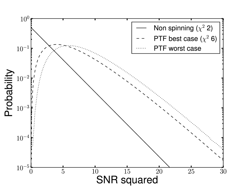
The SNR (9) for a non-precessing template follows a $\chi^{2}$ distribution with two degrees of freedom in Gaussian noise. This is also plotted on Figure 1. By comparing the distributions of the PTF and non-precessing SNRs, it is clear that the background triggers produced by the PTF search will have, on the average, considerably larger SNR than those produced by the non-precessing search. We explore the effect that this has on a search further in section 4.

3 Coherent Spinning PTF search

In this section, we introduce a multi-detector, coherent formulation of the PTF search. As in [22], we will restrict attention to the case where the sky location is known. This simplifies a coherent search as the sensitivity of the detectors to the two GW polarizations and the relative time delays between detectors are known. Astrophysically, this is of interest when searching for gravitational waves associated to electromagnetic transients such as GRBs [24, 26].

The data from various detectors are combined together coherently to form two coherent data streams, with one stream containing the $+$ polarization of any gravitational wave signal present in the network and the second containing the $\times$ polarization. The coherent method will offer an improvement in sensitivity over the coincidence method when more than two detectors are used, as only two data streams are searched. For networks with greater than two detectors, it is also possible to construct null streams which will contain no gravitational wave signal, and can be used as a consistency test [27, 22].

We begin by formulating the coherent SNR for the spinning PTF search and go on to explore how this will be distributed in Gaussian noise.

3.1 Coherent PTF Search Method

To formulate a coherent detection statistic for the PTF templates we draw on many of the methods and techniques that were used in deriving the single detector statistic described in section 2.1 and derived in detail in [14, 16]. We follow the conventions of [22] in extending this to a coherent, multi-detector search. Assuming that the noise in different detectors is independent, the multi-detector likelihood is given by

$$\ln\Lambda=(\mathbf{h}|\mathbf{s})-\frac{1}{2}(\mathbf{h}|\mathbf{h})$$ (11)

where we have defined a multiple detector matched filter

$$(\mathbf{a}|\mathbf{b})=\sum_{X}(a^{X}|b^{X}).$$ (12)

and the index $X$ runs over the detectors in the network.

As before, we want to maximize over as many of the parameters as possible to minimize the dimension of the required template bank. We start by maximizing this over the distance, D, and initial orbital phase, $\Phi_{0}$, to obtain

$$\ln\Lambda|_{\rm{max}(D,\Phi_{0})}=\frac{1}{2}\frac{\sum_{X,I}\left[\left(P_{I}^{X}A_{I}^{X}\right)^{2}+\left(P_{I}^{X}B_{I}^{X}\right)^{2}\right]}{\sum_{Y,J,K}\left[P_{J}^{Y}P_{K}^{Y}(Q_{0}^{J}|Q_{0}^{K})_{Y}\right]},$$ (13)

where $P_{I}$ are the amplitudes of the various waveform components $Q^{I}$, and $A_{X}^{I}$, $B^{I}_{X}$ are defined as in (5). Although the $P_{I}$ depend upon $D$ the maximized likelihood is independent of it as scaling the distance has an identical effect on both the numerator and denominator of eq. (13).

As in the single detector case, we would like to maximize over the $P_{I}$ to eliminate them. However, in the multi-detector case, they are detector dependent since the sensitivity of the detectors to the $+$ and $\times$ gravitational wave polarizations will differ. These sensitivities are encoded in the detector response functions, $F_{+}$ and $F_{\times}$, which depend on the sky location of the source in the detector frame. As we are focusing on an externally triggered search, where the sky location is known, these values will be known for each detector. We can then factor the detector dependent terms out of the $P_{I}^{X}$ as

$$P_{I}^{X}=F_{+}^{X}(\theta,\phi)S_{I}(D,\iota,\psi,\varphi_{0})+F_{\times}^{X}(\theta,\phi)T_{I}(D,\iota,\psi,\varphi_{0})$$ (14)

where $S_{I}$ and $T_{I}$ denote the amplitude of the $+$ and $\times$ components respectively of the 5 $Q_{I}$ in the radiation frame. They depend on the distance, $D$ and the angles $(\iota,\phi,\psi_{0})$ that describe the rotations necessary to transform from the source frame to the radiation frame.

We can re-cast the log-likelihood into a form which more closely resembles the single detector case by introducing ten-dimensional analogues of the $P_{I}$ and $Q^{I}$ by defining

$$\mathcal{P}_{\alpha} := \left[S_{1},S_{2},S_{3},S_{4},S_{5},T_{1},T_{2},T_{3},T_{4},T_{5}\right]$$

$$\mathcal{Q}_{0,\frac{\pi}{2}}^{\alpha} := \left[F_{+}Q_{0,\frac{\pi}{2}}^{1};...;F_{+}Q_{0,\frac{\pi}{2}}^{5};F_{\times}Q_{0,\frac{\pi}{2}}^{1};...;F_{\times}Q_{0,\frac{\pi}{2}}^{5}\right]\,.$$ (15)

The change to ten dimensions naturally arises because a multiple detector coherent network is sensitive to both the $+$ and $\times$ components, whereas a single detector network is only sensitive to one polarization. We also define the multi-detector inner products between signal and waveform components

$$\mathcal{A}^{\alpha} = (\mathbf{s}|\bm{\mathcal{Q}}_{0}^{\alpha})\quad\mbox{and}\quad\mathcal{B}^{\alpha}=(\mathbf{s}|\bm{\mathcal{Q}}_{\frac{\pi}{2}}^{\alpha})$$

$$\mathcal{M}^{\alpha\beta} = (\bm{\mathcal{Q}}_{0}^{\alpha}|\bm{\mathcal{Q}}_{0}^{\beta})=(\bm{\mathcal{Q}}_{\frac{\pi}{2}}^{\alpha}|\bm{\mathcal{Q}}_{\frac{\pi}{2}}^{\beta}).$$

The log likelihood equation can then be written as

$$\ln\Lambda|_{\rm{max}(D,\Phi_{0})}=\frac{1}{2}\frac{\mathcal{P}_{\alpha}\mathcal{P}_{\beta}\left(\mathcal{A}^{\alpha}\mathcal{A}^{\beta}+\mathcal{B}^{\alpha}\mathcal{B}^{\beta}\right)}{\mathcal{P}_{\alpha}\mathcal{P}_{\beta}\mathcal{M}^{\alpha\beta}}$$ (16)

We proceed, as before, by transforming to an orthonormal basis $\widetilde{\mathcal{Q}}_{0}^{\alpha},\widetilde{\mathcal{Q}}_{\frac{\pi}{2}}^{\alpha}$ for the waveform components. Then, maximizing freely over $\mathcal{P}_{\alpha}$ yields the coherent PTF SNR

$$\rho_{\mathrm{coh}}^{2}=\left[\widetilde{\mathcal{A}}\cdot\widetilde{\mathcal{A}}+\widetilde{\mathcal{B}}\cdot\widetilde{\mathcal{B}}\right]+\sqrt{\left(\widetilde{\mathcal{A}}\cdot\widetilde{\mathcal{A}}-\widetilde{\mathcal{B}}\cdot\widetilde{\mathcal{B}}\right)^{2}+\left(2\widetilde{\mathcal{A}}\cdot\widetilde{\mathcal{B}}\right)^{2}},$$ (17)

where, as before, the tilde denotes that we are in the orthonormal basis. This is very similar in form to the single detector statistic in equation (7). When the network is only sensitive to one polarization, the matrix $\mathcal{M}^{\alpha\beta}$ becomes degenerate and the maximization procedure must be re-visited. Here it is natural to remove all terms corresponding to the second polarization and reduce to 5 dimensions, as in the single detection search. Additionally, in section 2.1 we noted that when the template has no precession the single detection PTF SNR collapses to the familiar SNR formalism used in the non-spinning search. Similarly, in the coherent PTF search, when the template has no precession, the coherent SNR will collapse to the non-spinning coherent SNR given in [22].

The coherent SNR of equation (17) can be used as a detection statistic in performing a coherent search using PTF templates, as we explore in section 5. In the single detector search, we maximized freely over five $P_{I}$ which were dependent upon four physical parameters. Here, the $\mathcal{P}_{\alpha}$ still depend on only 4 parameters but we are now maximizing over ten amplitudes. This clearly introduces a lot of unnecessary freedom. We are currently investigating alternative methods of constructing the coherent SNR which might eliminate these un-physical degrees of freedom. However, we should note that the coincidence search allows for a similar freedom as the $P_{I}$ are maximized independently for each detector. Consequently, for a network with three or more detectors, the coherent search provides a sensitivity improvement.

3.2 SNR distribution in Gaussian noise

In section 2.2 we explored how the single detector PTF statistic is distributed in Gaussian noise. For the coherent PTF search we can use a similar strategy to investigate the distribution of the coherent SNR. In the coherent case there are twenty filters $\widetilde{\mathcal{A}}^{\alpha}$ and $\widetilde{\mathcal{B}}^{\alpha}$ and we have constructed the detection statistic such that $\widetilde{\mathcal{Q}}_{0}^{\alpha}$ and $\widetilde{\mathcal{Q}}_{\frac{\pi}{2}}^{\alpha}$ are orthonormal. As before, the only freedom is the relationship between the $0$ and $\frac{\pi}{2}$ terms encoded in

$$\widetilde{\mathcal{N}}^{\alpha\beta}=(\widetilde{\bm{\mathcal{Q}}}_{0}^{\alpha},\widetilde{\bm{\mathcal{Q}}}_{\frac{\pi}{2}}^{\beta}).$$ (18)

Figure 2: The “best” and “worst” possible distributions of the coherent PTF SNR squared as well as the distribution of the non spinning SNR squared.

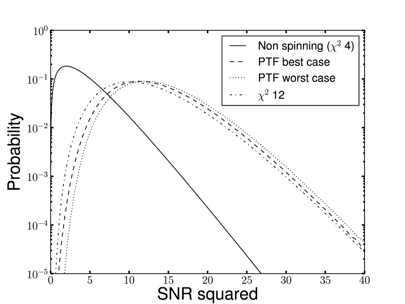
This is a 10x10 antisymmetric matrix comprised of four 5x5 blocks, each of which is antisymmetric. Therefore this matrix can have 8 non-zero eigenvalues: $\pm\lambda_{1,2,3,4}$. These eigenvalues determine the distribution of coherent SNR in Gaussian noise — for smaller eigenvalues, the large SNR tail of the distribution becomes more significant. In the tests that we have performed using the initial LIGO sensitivity curve and NSBH precessing templates, all four eigenvalues give values close to unity, the “best” case in which there are 12 independent waveform components. However, the distribution does not collapse to a $\chi^{2}$. In Figure 2, we demonstrate that this gives a distribution similar to a $\chi^{2}$ distribution with 12 degrees of freedom. In the “worst” case, where all of the eigenvalues are equal to 0, there are 20 independent waveform components and this distribution is also shown in Figure 2.

4 Identifying where the PTF search is most beneficial

In sections 2 and 3 we have derived the spinning SNR that can be used to perform a gravitational wave search using single spin inspiral waveforms as templates. We have demonstrated that, on the average, background triggers will have larger values of SNR in the PTF search than in the non-precessing search. At the same time, precessing PTF waveforms will be a better match to any spinning, precessing signals in the data. This begs the question as to whether it is preferable to use a search with non-precessing waveforms or single spin PTF waveforms to detect precessing systems. The PTF triggers will match the waveform better but this comes at the cost of searching a larger parameter space.

To quantify this, in Table 1 we give the SNR that corresponds to a false alarm probability (FAP) of $10^{-10}$ in Guassian noise for the various searches. We chose this value because it roughly corresponds to the loudest background events we observe when running the search on 2000 seconds of Gaussian noise, as is appropriate for a GRB search. The figures in the table show that the PTF search must obtain 26% more signal power (SNR squared) to be more efficient in the single detector case at this FAP and 38% more signal power for the coherent case.

	Non Precessing	PTF
Single detector	6.79	7.63
Coherent	7.26	8.53

Table 1: The SNR corresponding to a FAP of $10^{-10}$ for the non precessing and the PTF search, for both coherent and single detector cases. Here, for the PTF case the single detector and coherent detection statistics are assumed to be $\chi^{2}$ distributions with 6 and 12 degrees of freedom respectively.

There are large areas of the parameter space where precession will not significantly effect the evolution of the binary and thus a non-precessing template will pick up the majority of the power in a precessing signal. In these areas it would be better to search for the spinning signal with a non-precessing template, achieving a lower FAP than for the PTF search using an exactly matching template. Equivalently, when a system has little precession, the majority of power is contained in the $Q^{1}$ and $Q^{2}$ components of the PTF waveform and these two components are very similar, up to an overall phase shift. We can then consider performing a “restricted PTF” search, where we filter only these two components of the waveform against the data. This serves to reduce the FAP at a fixed SNR while losing only a small amount of the power in the signal.

To do this, we test every template waveform, before filtering, to determine whether on whether the template would be more likely to detect a matching signal below a false alarm probability of $10^{-10}$ using the restricted or full PTF search. This can be calculated by simulating a large number of gravitational wave signals, with masses and spin matching those of the template, but uniformly distributed in volume and orientation. Then, simply count the number of simulated signals expected to give an SNR greater than the value corresponding to a FAP $10^{-10}$ (given in Table 1) for both methods. Whichever of the PTF or restricted methods is expected to perform better is then used when filtering the data with that template. Using this method, we are able search the full parameter space of NSBH binaries in a single search, including non-spinning, non-precessing, marginally precessing and fully precessing configurations. This method works equally well for the single detector or the coherent search.

Figure 3: The fraction of templates analysed by the full PTF statistic as a function of the masses in the NSBH region of the parameter space.

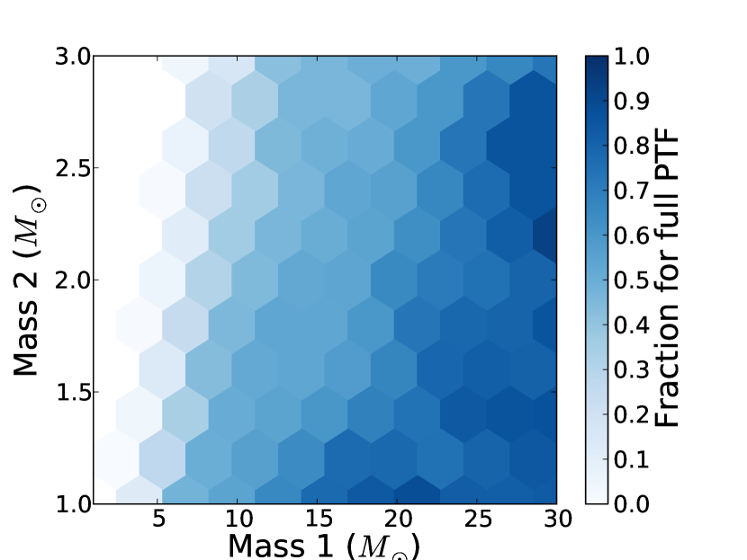
In Figure 3 we illustrate the fraction of templates analysed by the full PTF statistic, as a function of the masses, for the coherent search. The splitting of the templates into full and restricted does not require filtering against the data, but it does make use of the PSDs of the detectors. For this study, we use data from the three LIGO detectors during the S4 run.

A template bank was generating by taking a standard non-spinning template bank [28] in the mass space and, for each value of the masses, creating 15 templates with identical masses but spin parameters gridded over the two dimensional spin space, as described in [16]. The precessing single spin templates are most needed in the high mass ratio region of the parameter space. For this template bank, there are 35395 templates to be analysed with the restricted method and 14660 templates to be analysed with the full PTF method.

5 Search method and example results

In section 3 we derived a detection statistic appropriate for a coherent search using the PTF waveforms as templates. In section 4 we described a method through which one can identify where the PTF search is most needed and to split a template bank into those templates that should be analysed with the full PTF statistic and those that should be analysed with the restricted PTF statistic. We have combined these two methods together to create a search pipeline than can be used to coherently analyse gravitational wave data to search for precessing NSBH signals associated to short GRBs. We will briefly describe the analysis procedure before presenting an example result.

The search uses much of the same architecture as that described in [22] and [29]. Namely we search for gravitational wave signals in the “on-source” time, defined to be [-5,+1) seconds around the reported time of the GRB. Background is estimated from performing 324, 6 second trials around the GRB time, but at least 48s away from the on-source time. The coherent PTF search makes use of the same infrastructure as a coherent non-spinning search described in [22]. In particular, the data handling, PSD estimation and matched filtering routines are the same. Of course, the coherent PTF search makes use of spinning, precessing waveforms in the filtering and computes the SNR given in equation (17).

To demonstrate the performance of the coherent PTF, we ran it over a stretch of data from LIGOs S4 run. The data was chosen randomly, subject to the condition that all three of the LIGO detectors were operational at the time. This is the same data as was used to illustrate the template bank splitting in section 4, and the same bank with 15,000 full PTF and 35,000 restricted PTF templates was used.

Figure 4: The distribution of triggers found by the coherent PTF search. The left panels show the distribution of triggers from templates that were analysed using the “restricted” coherent PTF search, the right panels show the distribution from the templates that were analysed using the “full” coherent PTF search. The top panels were created from analysing Gaussian noise. The bottom panels were created from analysing a stretch of real data from S4. All these plots have been rescaled to use the same y-axis. For the two cases using real data the non-Gaussian spikes extend much higher than is shown, the loudest trigger has an SNR of 39 in the restricted case and 45 in the full case.

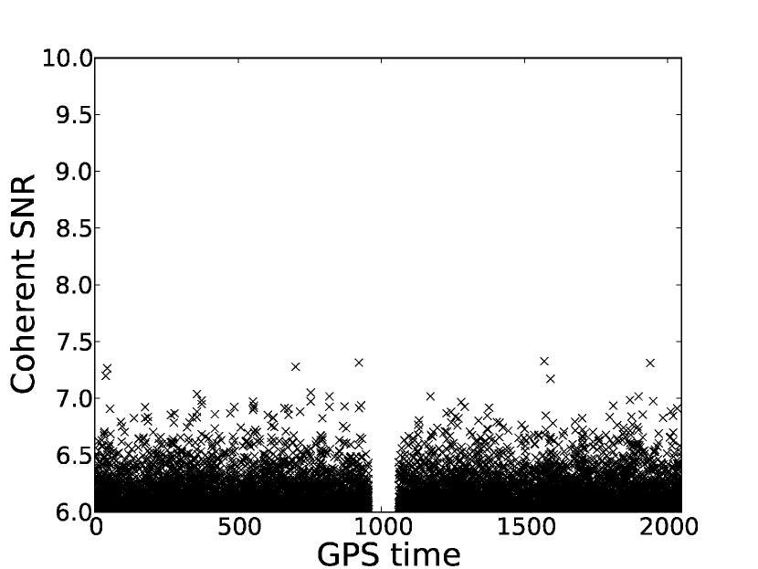
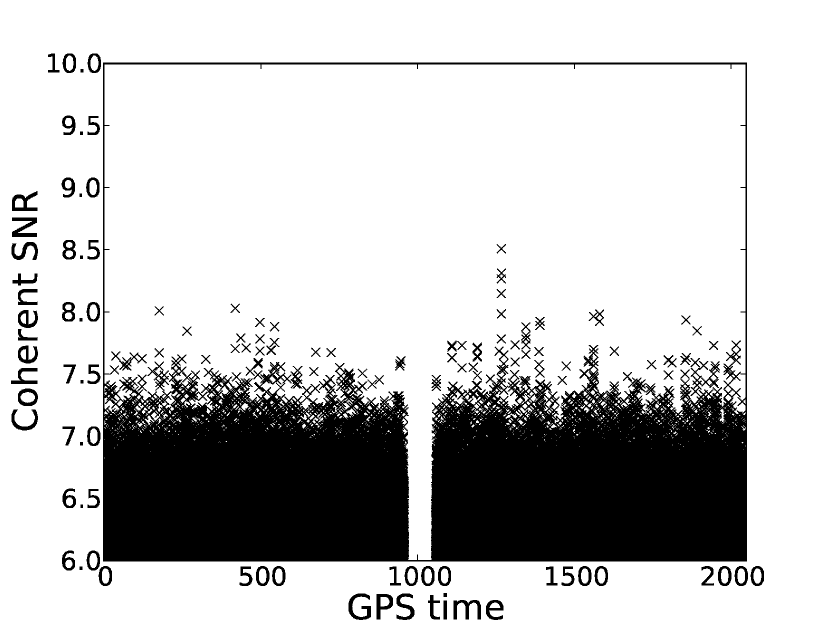
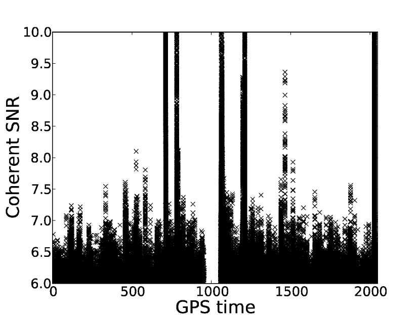
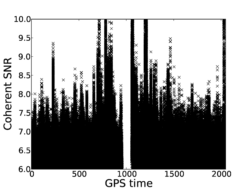
In Figure 4 we show the distribution of the SNR of the triggers produced using both the full and restricted statistic. This is shown for the stretch of real S4 data and for a stretch of simulated Gaussian data. As expected, the SNRs of triggers in Gaussian noise are larger for the precessing templates than the restricted ones, even though significantly fewer templates were analysed with the full statistic. The results from real data are badly affected by non-Gaussianities in the data. A number of loud transients are clearly visible as short duration peaks of large SNR, while there are an even greater number of quieter peaks throughout the analyzed time. This has a similar effect on both the full and restricted waveforms.

In [22], we described and developed a number of tools which can be used to effectively remove the majority of the non-Gaussian features from a non-spinning, coherent analysis. These include null stream consistency [27], amplitude consistency and $\chi^{2}$ signal consistency tests [13, 30]. All of these can be applied without modification to the restricted PTF search, and it seems reasonable to expect they would be similarly effective in reducing the effect of non-Gaussianities in the data. However, we currently have no such tools which can be used for the full PTF waveforms. Before using this search on real data we will need to implement a set of tests that can discriminate glitches from real signals for the full statistic. It should be relatively straightforward to implement the null stream consistency test. Unfortunately, as discussed in [22], the null stream for the LIGO S4 detectors is constructed only from the two instruments in Hanford. In this stretch of data the loudest background triggers are caused by non-stationarities in the Livingston detector and thus the null stream is ineffective. Alternatively a $\chi^{2}$ test such as the ones described in [13, 30] could be adapted to this search, [16] presents a possible way of doing this for single detectors. We are working on developing an alternative version of this $\chi^{2}$ test, which would test the consistency of the six independent components of a single detector PTF waveform, and then extending this to the fully coherent analysis.

6 Discussion

In this paper we have presented a method for performing a coherent search for precessing, single spin black hole–neutron star coalescences using the PTF method. We have compared the performance to searches using non-precessing waveforms and have identified regions of the parameter space where the PTF search offers increased sensitivity. We have presented a method by which these areas could be identified and demonstrated these techniques on a short stretch of S4 data.

This method should allow for the detection of highly precessing NSBH sytems with greater efficiency than the current non-spinning searches. However, more work is required before this search is ready to be used. The main need is for the development of effective methods of separating glitches from real events in the full PTF search, whether performing a coincident or a coherent search. As discussed in section 5, it should be possible to adapt a lot of the methods that have proven effective in non-spinning searches [7, 22] but this is a non-trivial task.

In this paper, we have focused on the PTF precessing waveforms. However, many of the techniques we have discussed would be equally applicable to the dominant harmonic of any family of precessing waveforms. In particular, the method of maximizing over freely over the amplitudes of the five components of the $l=2$ spin weighted-spherical harmonic is directly applicable to other waveform families. As the catalogue of numerical simulations of precessing binaries grows, these methods may well find applications in searches using such as numerical relativity inspired inspiral-merger-ringdown waveforms.

References

- [1] J. Abadie et al. Search for Gravitational Waves from Compact Binary Coalescence in LIGO and Virgo Data from S5 and VSR1. Phys. Rev., D82:102001, 2010.
- [2] B. P. Abbott et al. Search for Gravitational Waves from Low Mass Compact Binary Coalescence in 186 Days of LIGO’s fifth Science Run. Phys. Rev., D80:047101, 2009.
- [3] B. P. Abbott et al. Search for Gravitational Waves from Low Mass Binary Coalescences in the First Year of LIGO’s S5 Data. Phys. Rev., D79:122001, 2009.
- [4] Theocharis A. Apostolatos, Curt Cutler, Gerald J. Sussman, and Kip S. Thorne. Spin induced orbital precession and its modulation of the gravitational wave forms from merging binaries. Phys. Rev. D, 49:6274–6297, 1994.
- [5] Philippe Grandclement, Vassiliki Kalogera, and Alberto Vecchio. Searching for gravitational waves from the inspiral of precessing binary systems. I: Reduction of detection efficiency. Phys. Rev., D67:042003, 2003.
- [6] Kip S. Thorne. Gravitational radiation. In S.W. Hawking and W. Israel, editors, Three hundred years of gravitation, pages 330–458. Cambridge University Press, 1987.
- [7] Bruce Allen, Warren G. Anderson, Patrick R. Brady, Duncan A. Brown, and Jolien D. E. Creighton. FINDCHIRP: An algorithm for detection of gravitational waves from inspiraling compact binaries. 2005.
- [8] S. Babak, R. Balasubramanian, D. Churches, T. Cokelaer, and B. S. Sathyaprakash. A template bank to search for gravitational waves from inspiralling compact binaries. I: Physical models. Class. Quant. Grav., 23:5477–5504, 2006.
- [9] P. Ajith et al. Inspiral-merger-ringdown waveforms for black-hole binaries with non-precessing spins. 2009.
- [10] B. Abbott et al. Search of S3 LIGO data for gravitational wave signals from spinning black hole and neutron star binary inspirals. Phys. Rev., D78:042002, 2008.
- [11] A. Buonanno, Y. Chen, and M. Vallisneri. Detection template families for precessing binaries of spinning compact binaries: Adiabatic limit. Phys. Rev. D, 67:104025, 2003. Erratum-ibid. D 74, 029904(E) (2006).
- [12] Chris Van Den Broeck et al. Template banks to search for compact binaries with spinning components in gravitational wave data. Phys. Rev., D80:024009, 2009.
- [13] Bruce Allen. A time-frequency discriminator for gravitational wave detection. Phys. Rev., D71:062001, 2005.
- [14] Yi Pan, Alessandra Buonanno, Yan-bei Chen, and Michele Vallisneri. A physical template family for gravitational waves from precessing binaries of spinning compact objects: Application to single-spin binaries. Phys. Rev., D69:104017, 2004. Erratum-ibid. D74, 029905(E) (2006).
- [15] A. Buonanno, Y. Chen, Y. Pan, and M. Vallisneri. Quasiphysical family of gravity-wave templates for precessing binaries of spinning compact objects: Application to double-spin precessing binaries. Phys. Rev .D, 70(10), November 2004. Erratum-ibid. D 74, 029902(E) (2006).
- [16] Diego Fazi. Development of a physical-template search for gravitational waves from spinning compact-object binaries with LIGO. PhD thesis, Università di Bologna, 2009.
- [17] C. A. K. Robinson, B. S. Sathyaprakash, and Anand S. Sengupta. A geometric algorithm for efficient coincident detection of gravitational waves. Phys. Rev., D78:062002, 2008.
- [18] B. P. Abbott et al. Einstein@Home search for periodic gravitational waves in early S5 LIGO data. Phys. Rev., D80:042003, 2009.
- [19] Archana Pai, Sanjeev Dhurandhar, and Sukanta Bose. A data-analysis strategy for detecting gravitational-wave signals from inspiraling compact binaries with a network of laser-interferometric detectors. Phys. Rev., D64:042004, 2001.
- [20] Sukanta Bose, Archana Pai, and Sanjeev V. Dhurandhar. Detection of gravitational waves from inspiraling compact binaries using a network of interferometric detectors. Int. J. Mod. Phys., D9:325–329, 2000.
- [21] Sukanta Bose, Sanjeev V. Dhurandhar, and Archana Pai. Detection of gravitational waves using a network of detectors. Pramana, 53:1125–1136, 1999.
- [22] Ian Harry and Stephen Fairhurst. A targeted coherent search for gravitational waves from compact binary coalescences. 2010.
- [23] B. P. Abbott et al. Search for gravitational-wave bursts associated with gamma-ray bursts using data from LIGO Science Run 5 and Virgo Science Run 1. Astrophys. J., 715:1438–1452, 2010.
- [24] Ehud Nakar. Short-hard gamma-ray bursts. Phys. Rept., 442:166–236, 2007.
- [25] L A Wainstein and V D Zubakov. Extraction of Signals from Noise. Prentice-Hall, Englewood Cliffs, 1962.
- [26] Masaru Shibata and Keisuke Taniguchi. Merger of black hole and neutron star in general relativity: Tidal disruption, torus mass, and gravitational waves. Phys. Rev., D77:084015, 2008.
- [27] Y. Guersel and M. Tinto. Near optimal solution to the inverse problem for gravitational wave bursts. Phys. Rev., D40:3884–3938, 1989.
- [28] Thomas Cokelaer. Gravitational waves from inspiralling compact binaries: hexagonal template placement and its efficiency in detecting physical signals. Phys. Rev., D76:102004, 2007.
- [29] J. Abadie et al. Search for gravitational-wave inspiral signals associated with short Gamma-Ray Bursts during LIGO’s fifth and Virgo’s first science run. Astrophys. J., 715:1453–1461, 2010.
- [30] Chad. Hanna. Searching for gravitational waves from binary systems in non-stationary data. PhD thesis, Louisiana State University, 2008.