Detection of treatment effects by covariate-adjusted expected shortfall
Abstract
The statistical tests that are commonly used for detecting mean or median treatment effects suffer from low power when the two distribution functions differ only in the upper (or lower) tail, as in the assessment of the Total Sharp Score (TSS) under different treatments for rheumatoid arthritis. In this article, we propose a more powerful test that detects treatment effects through the expected shortfalls. We show how the expected shortfall can be adjusted for covariates, and demonstrate that the proposed test can achieve a substantial sample size reduction over the conventional tests on the mean effects.
doi:
10.1214/10-AOAS347keywords:
.TX1Supported in part by the National Science Foundation (USA) Award DMS-06-04229, National Institute of Health (USA) Grant R01GM080503-01A1, NNSF of China Grant 10828102, and a Changjiang Visiting Professorship at the Northeast Normal University, China.
, and
1 Introduction
We consider the problem of testing the hypothesis of no treatment effect against a class of alternatives where the two outcome distributions differ only or mainly in the right tail. As demonstrated in some recent trials of rheumatoid arthritis therapies in (2006) and (2006), the changes in Total Sharp Scores, the primary measurements of the treatment effects on prevention of structural damage, are nearly identical for most therapies for nearly 75% of the patient population, but the difference lies in the most challenging 25% of the patient population where a less effective treatment loses its efficacy, resulting in a heavy right tail in its outcome distribution. The two-sample -test or its regression counterpart in covariate-adjusted linear models is commonly used for detecting the treatment effects, but due to skewness and heavy-tails of the distributions, the test does not have satisfactory power. Nonparametric tests on the median differences, for example, would fare even worse in such cases, because the median differences are often negligible among those therapies.
A natural test in this type of applications is to focus on the average in one tail, or the expected tail loss (aka expected shortfall). In finance, this is often referred to as the conditional value at risk (CVaR), for measuring the risk of a portfolio. In our context, a treatment is said to be more effective if it has a smaller expected shortfall, where the expected shortfall is defined to be the conditional mean of the outcome (e.g., change in Total Sharp Score) above the th quantile. In this paper, will be taken to be a user-specified value (e.g., 0.75), but a good choice of clearly depends on the area of applications. In finance, the most relevant choices of fall above 0.90.
A two-sample comparison of the expected shortfalls is not difficult, as it falls into the well-known theory of the -statistic. In fact, there are also a large number of other tests that one can use to compare tails of two outcome distributions, but few have been developed to adjust for covariates. The purpose of this paper is to develop a simple test for testing the hypothesis on the treatment effect adjusting for certain covariates; the proposed test uses the COVariate-adjusted Expected Shortfall (COVES).
Our work starts with a brief introduction to our motivating example on the TSS for rheumatoid arthritis therapies in Section 2. In Section 3, we propose an appropriate treatment effect size of covariate-adjusted expected shortfall, followed by a new test for detecting differences in the treatment effects. The large sample theory for the proposed test is given here. In Section 4, we compare the proposed COVES test with the -test based on the least squares regression in empirical power. In particular, we show that when the outcome distributions resemble those of the TSS, the COVES test has a clear advantage in reducing sample sizes in clinical trials. The basic idea and methodology developed in this paper apply to other problems of comparing two covariate-adjusted tails of outcome distributions. In Section 5, we provide a diagnostic tool that can be used to gauge the need for the proposed test and to guide the selection of . Section 6 concludes the paper with some additional remarks about the COVES test.
2 A primer on total sharp scores
Rheumatoid arthritis (RA) is a chronic disabling disease that causes destruction of joint cartilage and erosion of adjacent bones. In RA clinical trials, TSS is used to measure the treatment effect of RA drugs on prevention of structural damage to the joints. It consists of two components, erosion score and score for joint space narrowing (JSN), which are obtained through examination of hand and/or feet joints with radiographic methods. The first description of TSS is given by (1971), but TSS has been modified in later studies. The example presented in this paper is based on van der Heijde’s modification of TSS scoring system [van der Heijde (2000)], which is based on examination of 16 areas for erosions and 15 for joint space narrowing in each hand. The erosion score per joint ranges from 0 to 5 with 0 representing a normal condition and 5 the most severe disease, and thus the total erosion score ranges from 0 to 160 (16 areas by 2 hands by 5). The JSN score ranges from 0 to 4 per joint with higher score representing more severe disease, which leads to a range of 0 to 120 (15 areas by 2 hands by 4) for the total JSN score. Therefore, the range of TSS is 0 – 280. The primary interest is the change from baseline in TSS in one or two years.
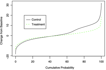
The change in TSS has a highly skewed distribution under any known treatment. In the TEMPO trial [(2006)] comparing Methotrexate, Etanercept, and the combination therapy of Etanercept and Methotrexate, the three treatments are similarly effective for about 75% of the patients whose conditions improved or showed no or little progression from the baseline; see Figure 1.

Medians for all three groups are around 0. Treatment differences come from the 25% of the patients with the most progressive diseases. In other words, the differences in treatment effects are not attributed to a location-scale change in the distributions. The distributions of clinical data from several other major RA trials [(2006); (2004); (2000)] showed similar characteristics.
It is clear that the distributions for the changes in TSS are far from normal, and the -test is expected to lose power due to skewness and heavier-tails that are evident in the data. Nonparametric tests on the median differences would fare even worse, because the median differences of those treatments are essentially nonexistent. Researchers in some trials have considered the chi-square tests on the proportion of patients with little disease progression by dichotomizing TSS, but there has been no agreeable cutoff point for dichotomization. In fact, the power of the chi-square test depends rather critically on the cutoff point. In addition, it is difficult to perform the chi-square test when a covariate needs to be adjusted for. A natural quantity for distinguishing treatment effects is the expected shortfall, which averages the changes in TSS in the upper tail. We propose to use the regression quantile approach of Koenker and Bassett (1978) to estimate the covariate-adjusted expected shortfall.
Later in this paper, we use a recent observational study conducted at Brigham and Women’s Hospital and sponsored by Millennium Pharmaceuticals Inc. and Biogen Idec as a basis for assessing the performance of the proposed test. We take 150 subjects in the study, who are under active treatment, and simulate a control group whose outcome distribution is chosen to mimic the treatment difference reported in other trials. For example, in the Adalimumab trial [(2004)], the variance of the treatment group (using the drug Adalimumab 20 mgkg) is about half of that in the control group (using the drug Methotrexate) with a mean difference of . In the Abatacept trial [(2006)], the variance in the Abatacept group is about one third of that in the control group. In our simulation studies, we use the ratio of variances between 2:1 and 3:1 between two treatment groups.
3 Proposed test: COVES
We use a dummy variable as treatment indicator, as the covariate of interest, and as the outcome measure. For simplicity of notation, we consider as a univariate covariate and taking values 0 or 1, but the work generalizes readily for multivariate covariates and multiple treatments. As appropriate with randomized trials, we assume that and are independent. We model the th quantile of given as
| (1) |
where the coefficients , and are -specific. In this paper, we use for empirical studies, but refer to Section 5 for guidance on the selection of . We also refer to Koenker (2005) for details on the linear regression quantile specification.
Given data with for and for , we can use the quantreg package in R to obtain the regression quantile coefficient , , and . Then, let as the residuals from the th regression quantile. By contrast, we also write , which has zero as the th conditional quantile given () due to (1).
Let be the covariate-adjusted outcome, and define the empirical covariate-adjusted expected shortfall for the two groups as
where and . The quantity is the average of the outcomes for group that are above the th covariate-adjusted quantile.
The proposed test statistic for the hypothesis of no difference between the two treatment groups is given as
| (2) |
Let and be the average of and in group that are above the th regression quantile, that is,
Then, the test statistic (2) can be written as
| (3) |
which makes it relatively easy to establish the asymptotic normality of the test statistic as .
To estimate the variance of , let , be the conditional density function of given evaluated at 0, and
as the orthogonal components relative to the treatment groups. In more general problems, we can obtain by the Gram–Schmidt orthogonalization of the design matrix. Furthermore, let
and
| (4) | |||
Theorem 3.1
Suppose that exists, , and are uniformly bounded away from 0 and infinity. Under the null hypothesis that , we have
The proof of Theorem 3.1 is given in the Appendix, but to use the asymptotic normality for testing the null hypothesis of no treatment effects, we need a consistent estimate of . If in each group (corresponding to or 1) follows a common distribution, then a kernel density estimate can be used to estimate the common density at 0 from in the th group. If the conditional densities vary with , it is not possible to estimate each consistently, but , a linear combination of the ’s, can still be consistently estimated; see (2002) and Koenker (2005) for more details. For the empirical investigations in this paper, the proposed test is carried out using a kernel density estimate, density, in R on each treatment group.
4 Empirical investigations
In this section, we report some empirical power studies of the proposed test based on Monte Carlo simulations. The first study is constructed based on the data we obtained from a recent study on an undisclosed therapy to treat RA at the Brigham and Women’s Hospital in Boston. The other studies are constructed with other types of distributions in mind. Together, we find that the proposed test greatly outperforms the usual regression tests on the mean differences when the group differences occur at one tail of the distributions.
4.1 Targeted study on TSS
We use the empirical distributions, , of the TSS changes of 150 patients in the Brigham and Women’s Hospital study as the underlying distribution for the group . We take the baseline TSS as the covariate in the analysis, whose empirical distribution for the group will be denoted as .
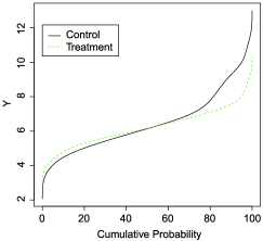
The data from the control group (with ) will be simulated as
where is a uniform random number in (0, 1). Clearly, the control group has a heavier right tail in its outcome, but the covariate has the same distribution in both groups. In this setting, the variance of the control group is about twice that of the treatment group. Table 1 and Figure 2 summarize the differences of the two groups.
| 0.5 | 0.6 | 0.7 | 0.75 | 0.8 | 0.9 | 0.99 | Mean | Variance ratio | |
|---|---|---|---|---|---|---|---|---|---|
| 0 | 0 | 3.72 | 4.53 | 4.96 | 5.64 | 6.02 | 1.74 | 2.03 |

The power functions for the test with and the -test from linear regression are shown in Figure 3 with sample sizes up to . For comparison, we also include in the figure the power curve for the test based on expected shortfalls (ES) without adjusting for the baseline TSS. Table 2 provides the sample sizes needed to reach a power of 0.90 in clinical trials with as well as . It is common in clinical experiments to allocate twice as many patients to the treatment group when the treatment is believed to be effective. In this case, the baseline TSS does not play a significant role, so the statistical power for detecting the treatment effect has no gain by adjusting the covariate in the analysis. However, the results show that the COVES test is clearly outperforming the -test, and the latter would require a trial that is more than double in size.
=210 pt Sample size test () (120, 120) or (172, 86) -test (306, 306) or (450, 225)
4.2 More simulation studies
We consider data generated from
| (5) |
where , and is either 0 (under the null hypothesis) or 1.35 (under the alternative hypothesis). The coefficient and the distribution for the covariate will be specified later. Clearly, the control group () has a heavier right tail. When , the error variance of the control group () is about triple that of the treatment group () under this model. Table 3 summarizes the differences of the two groups under the alternative hypothesis.
=270 pt 0.5 0.6 0.7 0.75 0.8 0.9 Mean Var ratio 0 0.34 0.70 0.91 1.13 1.72 0.54 2.97
We will consider four scenarios for the effects of the covariate in the analysis:
-
•
Scenario 1, no covariate effect: we take from , with .
-
•
Scenario 2, a common covariate effect: we take from , with .
-
•
Scenario 3, a covariate distribution that varies with treatment groups: we take from for , but from for , with .
-
•
Scenario 4, a covariate distribution that has a scale change across treatment groups: we take from for , but from for , with .
Scenarios 3 and 4 are unlikely for randomized trials, but we include them in the study to examine the robustness of the test when the covariate distributions vary to some extent with the treatment groups. The type I errors of the test and the -test under these scenarios are controlled to stay close to the nominal level of 0.05. The following table reports the type I errors at the sample size of . It also reports the sample sizes needed to reach power of 0.90 in each scenario under two design conditions: and , respectively.
| test | t-test | |||
|---|---|---|---|---|
| Type I error | Sample size | Type I error | Sample size | |
| needed to reach | needed to reach | |||
| Scenario | (50, 50) | power 0.9 | (50, 50) | power 0.9 |
| 1 | 0.046 | (51, 51) or (92, 46) | 0.050 | (140, 140) or (202, 101) |
| 2 | 0.051 | (51, 51) or (92, 46) | 0.049 | (140, 140) or (202, 101) |
| 3 | 0.048 | (59, 59) or (100, 50) | 0.050 | (177, 177) or (240, 120) |
| 4 | 0.053 | (50, 50) or (92, 46) | 0.052 | (140, 140) or (200, 100) |
 |
 |
| (a) | (b) |
|
|
| (c) | |
The results clearly show the efficiency of the test. In Scenarios 2–4, the adjustment of the covariate is important, because the ES test considered in Section 4.1 would not be valid, and thus it is not presented in this subsection.
5 A diagnostic tool for
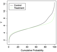
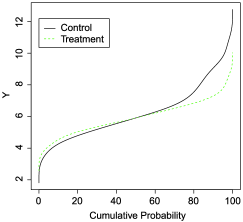
When preliminary or full data are available, it is often helpful to have a simple diagnostic tool that points to a case in favor of the test. We suggest examining the quantile function plot, as used in Figure 1, but applied to the covariate-adjusted outcomes defined in Section 3. When the quantiles of covariate-adjusted outcomes from different treatment groups differ mostly in one tail, we have a clear case in favor of the test or a similar test that focuses on the tail. In fact, the plot can also suggest an appropriate level of to be used for . To illustrate this point, we simulated one data set of size from Scenario 3 in Section 4.2 with in model (5). Unsure about a good choice of , we considered using the covariate-adjusted outcomes from three quantile levels 0.5, 0.75, and 0.9, and examined the resulting quantile plots in Figure 4. No matter which quantile level we started with, the quantile plots of the covariate-adjusted outcomes look similar, and they all suggest that the test with around 0.75 would be a good choice. On the other hand, if the quantile functions of different treatment groups show a vertical shift, we would then favor the -test to the test.
6 Conclusions
The proposed test aims to detect treatment effects that are reflected mostly in the upper (or lower) tail of the outcome distributions. The test is powered up by the use of the expected shortfall as a natural differentiating quantity in such applications. We find that the regression quantile methodology is appropriate and convenient for computing the covariate-adjusted expected shortfall in the test. Our study on the change of the Total Sharp Scores due to different treatments on rheumatoid arthritis shows that a substantial sample size reduction over the conventional t-test based on linear models can be achieved.
In this paper, we used in the proposed test, because it serves two purposes in the application. First, earlier studies have shown conventional rheumatoid arthritis treatments are effective for nearly 75% of the patient population, so it is less meaningful to detect differences below the 75th percentile. Second, a more effective treatment should work well for a substantial portion of the patients, so if we set to be too high in the test, a significant difference in the upper tail might be difficult to detect statistically. Finally, we note that the development of the test in this paper was made in response to the randomized clinical studies on rheumatoid arthritis treatments, but the basic idea and the methodology clearly generalize to other problems (where tail differences of possibly other values are) of interest. In general, we suggest using quantile function plots on covariate-adjusted outcomes as a simple diagnostic tool for suggesting a good choice of .
Appendix: Sketch of proof
The following lemma follows directly from the consistency and the Bahadur representation of regression quantile estimators; see Koenker [(2005), Section 4.3] and (1996).
Lemma 1
If is a random sample satisfying (1), exists, , and are uniformly bounded away from 0 and infinity, then we have the Bahadur representation on
and the representation on
where is the conditional density function of given evaluated at 0, and
References
- (1) He, X., Fung, W. K. and Zhu, Z. Y. (2002). Estimation in a semiparametric model for longitudinal data with unspecified dependence structure. Biometrika 89 579–590. \MR1929164
- (2) He, X. and Shao, Q. M. (1996). A general Bahadur representation of M-estimators and its application to linear regression with nonstochatic designs. Ann. Statist. 24 2608–2630. \MR1425971
- (3) Keystone, E. C., Kavanaugh, A. F., Sharp, J. T., Tannenbaum, H., Hua, Y., Teoh. L. S., Fischkoff, S. A. and Chartash, E. K. (2004). Radiographic, clinical, and functional outcomes of treatment with adalimumab (a human anti-tumor necrosis factor monoclonal antibody) in patients with active rheumatoid arthritis receiving concomitant methotrexate therapy: A randomized, placebo-controlled, 52-week trial. Arthritis Rheum. 50 1400–1411.
- Koenker and Bassett (1978) Koenker, R. and Bassett, G. (1978). Regression quantiles. Econometrica 46 33–50. \MR0474644
- Koenker (2005) Koenker, R. (2005). Quantile Regression. Cambridge Univ. Press. \MR2268657
- (6) Kremer, J. M., Genant, H. K., Moreland, L. W., Russell, A. S., Emery, P., Abud-Mendoza, C., Szechinski, J., Li, T., Ge, Z., Becker, J. and Westhovens, R. (2006). Effects of abatacept in patients with methotrexate-resistant active rheumatoid arthritis. A randomized trial. Ann. of Internal Medicine 144 865–876.
- (7) Lipsky, P. E., Van Der Heijde, D., St. Clair, E. W., Furst, D. E., Breedveld, F. C., Kalden, J. R., Smolen, J. S., Weisman, M., Emery, P., Feldmann, M., Harriman, G. R. and Maini, R. N. (2000). Infliximab and methotrexate in the treatment of rheumatoid arthritis. N. Engl. J. Med. 343 1594–1602.
- (8) Sharp, J. T., Lidsky, M. D., Collins, L. C. and Moreland, J. (1971). Methods of scoring the progression of radiologic changes in rheumatoid arthritis. Correlation of radiologic, clinical and laboratory abnormalities. Arthritis Rheum. 14 706–720.
- van der Heijde (2000) van der Heijde, D. (2000). How to read radiographs according to the Sharp/van der Heijde method. J. Rheumatol. 27 261–263.
- (10) van der Heijde, D., Klareskog, L., Rodriguez-Valverde, V., Codreanu, C., Bolosiu, H., Melo-Gomes, J., Tornero-Molina, J., Wajdula, J., Pedersen, R., Fatenejad, S. and TEMPO Study Investigators (2006). Comparison of etanercept and methotrexate, alone and combined, in the treatment of rheumatoid arthritis. Arthritis Rheum. 54 1063–1074.