An imputation-based approach for parameter estimation in the presence of ambiguous censoring with application in industrial supply chain

Abstract

This paper describes a novel approach based on “proportional imputation” when identical units produced in a batch have random but independent installation and failure times. The current problem is motivated by a real life industrial production–delivery supply chain where identical units are shipped after production to a third party warehouse and then sold at a future date for possible installation. Due to practical limitations, at any given time point, the exact installation as well as the failure times are known for only those units which have failed within that time frame after the installation. Hence, in-house reliability engineers are presented with a very limited, as well as partial, data to estimate different model parameters related to installation and failure distributions. In reality, other units in the batch are generally not utilized due to lack of proper statistical methodology, leading to gross misspecification. In this paper we have introduced a likelihood based parametric and computationally efficient solution to overcome this problem.

1 Introduction: Background of the problem.

After the production process, consumer goods are often distributed through multi-step channels, giving rise to the term “production–delivery” supply chain. An exception to this practice is “just-in-time” manufacturing where a product is assembled and shipped directly only upon the request of a customer, which is quite popular in the personal computer industry. However, for most consumer products, items produced by a company are not shipped directly to the final customer. The traditional route for any large scale industrial operation is to ship the manufactured products to a warehouse. The warehouses are often maintained by third party retailer/shops, from where the products are sold and installed at a future date to the final customer. Due to geographic as well as company–retailer relationship, once the batch is shipped, it is often unknown to the producing company whether a specific unit is working or is still not installed, until and unless the unit stops working and the final customer claims a warranty at a future date. At that point in time the data on the failed unit becomes “complete” in a sense that we know exactly its installation as well as failure time. For all other units it is not known (hence “partial” information only) whether they are working or are not at all installed. The above setup is quite common in practice in many industrial supply chains, giving rise to a situation where in-house engineers face a dilemma regarding the optimal usage of available information. The untimely failure of a unit is always costly to the producer from the warranty perspective [Abernethy (1996)]. Also, after infant mortality, reliability assessment and future lifetime prediction at an early stage of the product lifespan is advantageous for appropriate customer satisfaction issues.

Reliability estimation requires knowledge of the population at risk and the reliability of each unit of the population. The major objective is always to acquire timely information of interest on failure modes. However, in the presence of both “complete” and “partial” information, current practice is to estimate relevant reliability information by using those units which have completed their life cycle (i.e., “complete” portion only), while not utilizing the “partial” information [Abernethy (1996); Kececioglu (1993)]. The primary reason for this is the absence of any established methodology for dealing with the current situation. This clearly makes the inferential procedure suboptimal. In this article we adopt a proportional imputation based approach to yield a practical solution to the situation described above. The thrust of this paper is the estimation of the unknown parameters under the assumption that we know the actual parametric distribution of installation as well as failure time. The more general problem of unknown distributional form for either installation or failure time (or both) is not considered here and is left for future work.

The rest of the article is organized as follows. In the first three sections we present notation and a theoretical justification of the proposed methodology. Section 5 presents the algorithm for proportional imputation. The connection between the exact likelihood based approach and our proposed algorithm is described in Section 6. Section 7 describes the simulation performance of our algorithm. We also include the analysis of industrial furnace data in Section 8. We conclude the article with some discussion.

2 Notation and mathematical setting.

The problem of interest is motivated from a large industrial company producing residential furnace components. The units are produced and shipped within the continental USA via multiple channels. However, the general description of the problem and our solution is neither dependent on a specific company nor confined to a specific commodity. Rather, our proposed solution will have a broader application since the setup is common to many production delivery supply chains. Consider a setup in which $N$ identical units are produced in a batch, which are then shipped to a warehouse. These units will be installed only after being purchased by the customer at some future date. We assume there exists no substantial time lag between purchase and actual installation of unit/units. Purchase and installation will be considered as the event of interest, and the time in which this transpires will be referred to as the “installation time.” Consider a fixed end of study time $T_{0}$. The general data description at hand is rather simple. For a particular unit we either know both the installation and failure times or know nothing at all. In fact, for many units at time $T_{0}$, their current status will be unknown due to the fact that they have not yet failed either due to noninstallation or are still in working condition. Let $X$ $(\sim F_{X}(\cdot))$ and $T$ $(\sim F_{T}(\cdot))$ denote the continuous random variables corresponding to installation time and failure time and which are assumed to be independent of each other. In this paper we assume that $F_{X}(\cdot)$ and $F_{T}(\cdot)$ are completely specified but with unknown parameters. We denote the random set $\Omega=\{i\in\{1,2,\ldots,N\}\dvtx X_{i}+T_{i}\leq T_{0}\}$ to be the set of indices of the completely observed units. Let $C$ denote the cardinality of $\Omega\dvtx C=|\Omega|=\sum_{i=1}^{N}I\{X_{i}+T_{i}\leq T_{0}\}$. Following standard results in survival/reliability analysis, the complete likelihood for the above setup is

$$\hskip 8.5pt\qquad L(F_{X},F_{T}) = \prod_{i=1}^{N}[f_{X,T}(x_{i},t_{i})I\{x_{i}+t_{i}\leq T_{0}\}]^{\tau_{i}}[P\{X+T>T_{0}\}]^{1-\tau_{i}}$$

$$\propto \biggl{\{}\prod_{i\in\Omega}f_{X,T}(x_{i},t_{i})\biggr{\}}\biggl{\{}S_{X}(T_{0})+\int_{0}^{T_{0}}S_{T}(T_{0}-x)\,dF_{X}(x)\biggr{\}}^{N-C},\!\!\!\!\!\!\!\!\!$$

where $\tau_{i}$ is an indicator of whether the $i$th unit is observed or not for $i=1,2,\ldots,N$. The above likelihood is difficult to maximize numerically except for the very restrictive case when $X$ and $T$ are independent and identically distributed (i.i.d.) according to an exponential distribution. For the other popular reliability distributions (e.g., Weibull, Gamma), the above likelihood is difficult to maximize due to excessive flatness, especially when $C\ll N$. In the furnace data described in Section 8 and also in other simulation studies, the $\frac{C}{N}$ ratio is on average $40\%$ or below. With only this much data the above likelihood essentially becomes very flat and brute force optimization often produces unstable estimates with large variances. For more details on this see the simulation studies in Section 7. Next we provide a proportional imputation scheme that has close connection with the above likelihood, yet it employs a search strategy parallel to Monte-Carlo-based approaches which is computationally faster and produces stable estimates.

2.1 Standard practice and an alternative formulation.

For notational simplicity and without loss of generality, we assume that the first $C$ units are observed or, in other words, we have complete information for $\{x_{i},t_{i}\}_{i=1}^{C}$. Notably, the manufacturer knows nothing about a unit under two circumstances. First, if $X>T_{0}$, that is, the unit is not being installed until time $T_{0}$ and denoted as event $B$. Second, $X<T_{0}$ but $T>T_{0}-X$, that is, the unit is installed but still in operation and denoted as event $D$. Since exact likelihood is difficult to use, traditional practice is of two forms [Abernethy (1996); Kececioglu (1993)]. The most simplistic approach is to think that only $C$ units are produced. Since we will have complete information for all of them, we may use standard theory to estimate model parameters corresponding to $X$ and $T$ under specific distributional choices. The other practice is to think that we have $C$ units not from the full distribution but rather from the truncated distribution of both $X$ and $T$ (i.e., observed if $X<T_{0}$ and $T<T_{0}$). Then under some specific distributional assumptions (popular choices are Exponential, Weibull, etc.) the MLE or rank egression based approaches are used for parameter estimation [Wang (2004); Johnson (1964); Michael and Schucany (1986)]. Both of these approaches will produces erroneous estimates for the setup considered. The situation will be much simpler if it is also known for a specific “noninformative” unit whether it is under the event $B$ or $D$. This knowledge, if available, will enable us to render the case as Type-1 right censoring at $T_{0}$ either on $X$ (under $B$) or on $T$ (under $D$) and then follow the usual theory of estimation with censored data [Meeker and Escobar (1998); Klein and Moeschberger (2005)]. Unfortunately, practical considerations suggest that even this information will not be available under most producer–retailer setups resulting in “ambiguous” censoring. This is unavoidable unless the producer company has an agreement with the retailer to get in-time unit specific sales information. This involves monetary implications and often short-term cost cutting actions get higher priority.

In this article we took an alternative route to impute the installation time ($X$) for those units under $D$, that is, installed but not failed. Note that if we know or can successfully impute the installation time and assume that the unit is still working, this essentially means the failure time is being censored. This enables us to use standard methodology to estimate the model parameters [see Meeker and Escobar (1998); Klein and Moeschberger (2005)]. However, the crucial question is not only how to impute the unobserved installation time, but also how many units are needed to be imputed. Next we present the theory of an interesting computational approach to achieve this task based on a proportional sampling imputation scheme.

3 How many to sample and where to sample from?

In the parametric setup we generally assume some distributional form for $X$ and $T$, Weibull and Exponential being the most popular choice to reliability engineers [Abernethy (1996)]. Our present methodology is general in the sense that it does not depend on any specific distributional choice for both $X$ and $T$. Note that for $C$ complete units we have samples from three conditional distributions, namely:

1. []

2. $x|X+T\leq T_{0}$;

3. $t|X+T\leq T_{0}$;

4. $x+t|X+T\leq T_{0}$.

It is not difficult to formalize an estimation procedure if we have samples from $\{x|X\leq T_{0}\}$. However, the identity

$$f_{X}(x|X+T\leq T_{0})=\frac{f_{X}(x|X\leq T_{0})F_{T}(T_{0}-x)F_{X}(T_{0})}{F_{T+X}(T_{0})}$$

implies

$$f_{X}(x|X\leq T_{0}) = \frac{f_{X}(x|X+T\leq T_{0})F_{T+X}(T_{0})}{F_{T}(T_{0}-x)F_{X}(T_{0})}$$

$$\propto f_{X}(x|X+T\leq T_{0})F_{T}^{-1}(T_{0}-x)$$

$$\propto f_{X}(x|X+T\leq T_{0})\{1-S_{T}(T_{0}-x)\}^{-1}.$$

Note that the number of samples (if available) from $\{x|X\leq T_{0}\}$ will be larger than that from $\{x|X+T\leq T_{0}\}$. Hence, we have the identity, $\#\mbox{ samples }\{x|X\leq T_{0}\}-\#\mbox{ samples }\{x|X+T\leq T_{0}\}=\#\mbox{ samples }\{x|X\leq T_{0}\cap T>T_{0}-X\}$. We will try to impute this difference (or unobserved installations) via proportional sampling.

The above calculation shows why the assumption that the samples are from right truncated and independent distributions is not valid. Even though $X$ and $T$ are assumed to be independent, the very nature of the “installation-failure” setup will make them intrinsically dependent. Hence, it will be wrong to carry out separate estimation of the parameters of the distributions of $X$ and $T$ under the truncation assumption, as in reality we do not have samples from $\{x|X\leq T_{0}\}$ and $\{t|T\leq T_{0}\}$. Next we have exploited this mutual dependence of $X$ and $T$ via a sampling and imputation based approach.

3.1 Proportional imputation scheme.

To estimate the number of imputations necessary, let us denote the random variable $V=\sum_{j=1}^{N}V_{j}$, where

$$V_{j}=\cases{1,&\quad$\mbox{if $j${th} unit is installed on or before }T_{0},$\vspace*{2pt}\cr 0,&\quad$\mbox{otherwise.}$}$$

Hence, $P[V_{j}=1]=P[X\leq T_{0}]=F_{X}(T_{0})$ and $V_{j}\sim\operatorname{Bernoulli}(F_{X}(T_{0}))$.Under the assumption that units are identical and independent, $V\sim\operatorname{Binomial}(N,\break F_{X}(T_{0}))$. Hence, $E[V]=NF_{X}(T_{0})$ and since $C$ units are already observed, we need to impute for $NF_{X}(T_{0})-C$ units. Of course, $NF_{X}(T_{0})-C$ need not be an integer and so we round it up to produce a sensible estimate. We use $[\cdot]$ notation to denote this rounding procedure. All these make sense provided we know the parameters in $F_{X}(\cdot)$, but, in fact, the main purpose of this paper is to estimate those parameters. However, for the time being let us assume that some crude estimates of these parameters are available. We will describe exactly how to get such accurate estimates in Section 5.

Figure 1: Schematic diagram of $C$ observed installations.

Without loss of generality, we assume $C$ units are ordered in the sense that $x_{i}<x_{i+1}$ for $i=1,\dots,C-1$. The observed installations are depicted in Figure 1. These installations produce a natural $C+1$ partitioning of the study interval, that is, $[0,T_{0}]$. Due to the continuous distributional choice for $X$, we consider the case with no ties. However, we remark that the case with ties can be handled with minor modifications. The probability of a unit being installed in the interval $[x_{k},x_{k+1}]$ is given by $P[x_{k}<X<x_{k+1}]=F_{X}(x_{k+1})-F_{X}(x_{k})$. An installed unit will remain unobserved if it does not fail by $T_{0}$. So the conditional probability of remaining unobserved is given by

$$P[T>T_{0}-X|x_{k}<X<x_{k+1}]=\frac{\int_{x_{k}}^{x_{k+1}}S_{T}(T_{0}-x)f_{X}(x)\,dx}{F_{X}(x_{k+1})-F_{X}(x_{k})}.$$ (3)

Next we present a theorem for the above conditional probability if the interval $[x_{k},x_{k+1}]$ becomes narrower, that is, $x_{k+1}\downarrow x_{k}$.

Theorem 3.1.

$\lim_{x_{k+1}\downarrow x_{k}}\frac{\int_{x_{k}}^{x_{k+1}}S_{T}(T_{0}-x)f_{X}(x)\,dx}{F_{X}(x_{k+1})-F_{X}(x_{k})}=S_{T}(T_{0}-x_{k})$, provided $f_{X}{(x_{k+1})}\neq 0$.

This follows by application of l’Hospital’s rule. This indicates that if $x_{k+1}\downarrow x_{k}$, then the probability of survival (i.e., remaining unobserved) for a unit installed exactly at $x_{k}$ will be $S_{T}(T_{0}-x_{k})$.

Now using equation (3), the joint probability of a unit being installed in $[x_{k},x_{k+1}]$ and then remaining unobserved is

$$\qquad P[(x_{k}<X<x_{k+1})\cap(T>T_{0}-X)]=\int_{x_{k}}^{x_{k+1}}S_{T}(T_{0}-x)f_{X}(x)\,dx.$$ (4)

Due to the nonincreasing property of the survival function, it is easy to see that

$$S_{T}(T_{0}-x_{k})\int_{x_{k}}^{x_{k+1}}f_{X}(x)\,dx \leq \int_{x_{k}}^{x_{k+1}}S_{T}(T_{0}-x)f_{X}(x)\,dx$$

$$\leq S_{T}(T_{0}-x_{k+1})\int_{x_{k}}^{x_{k+1}}f_{X}(x)\,dx.$$

We would like to use the above inequality to approximate equation (4) via

$$I_{k+1} = P[(x_{k}<X<x_{k+1})\cap(T>T_{0}-X)]$$

$$\simeq \frac{S_{T}(T_{0}-x_{k})+S_{T}(T_{0}-x_{k+1})}{2}[F_{X}(x_{k+1})-F_{X}(x_{k})].$$

Note if $T_{0}\downarrow$ but $[x_{k},x_{k+1}]$ remains fixed with $x_{k+1}\leq T_{0}$, then $I_{k+1}\uparrow$ due to the monotone decreasing property of the survival function. Conversely, if $T_{0}\uparrow$, then $I_{k+1}\downarrow$. The approximation for $I_{k+1}$ given in equation (3.1) works very well provided the observed installation times are not very sparse over $[0,T_{0}]$. Next, we present a theorem characterizing unobserved installation times over different regions.

Theorem 3.2.

Let $x_{k}\in(x_{k-1},x_{k+1})$. Then $P[T>T_{0}-X|x_{k-1}<X<x_{k}]\leq P[T>T_{0}-X|x_{k}<X<x_{k+1}]$.

The proof is provided in the Appendix. Theorem 3.2 implies that the probability of remaining unobserved increases as the installation time gets closer to the end of study time $T_{0}$. Equation (3.1) characterizes the probability of a single unit being installed in $[x_{k},x_{k+1}]$ but remains unobserved until $T_{0}$. Note that we have $C+1$ such intervals in $[0,T_{0}]$. Hence, the expected number of unobserved installations in $[x_{k},x_{k+1}]$ is

$$\alpha_{k+1}=\frac{\{NF_{X}(T_{0})-C\}I_{k+1}}{\sum_{j=0}^{C}I_{j+1}},$$

with the identity $\sum_{k=0}^{C}\alpha_{k+1}=NF_{X}(T_{0})-C$.

Lemma 3.1.

$\sum_{k=0}^{C}I_{k+1}=\sum_{k=1}^{C}\frac{F_{X}(x_{k})}{2}[S_{T}(T_{0}-x_{j-1})-S_{T}(T_{0}-x_{j+1})]+F_{X}(T_{0})\frac{1+S_{T}(T_{0}-x_{c})}{2}$, where $x_{0}=0$ and $x_{C+1}=T_{0}$.

Note that $I_{k+1}=\frac{S_{T}(T_{0}-x_{k})+S_{T}(T_{0}-x_{k+1})}{2}[F_{X}(x_{k+1})-F_{X}(x_{k})]$. Hence,

$$\sum_{k=0}^{C}I_{k+1} = \sum_{k=0}^{C}\frac{S_{T}(T_{0}-x_{k})+S_{T}(T_{0}-x_{k+1})}{2}[F_{X}(x_{k+1})-F_{X}(x_{k})]$$

$$= [F_{X}(x_{1})-F_{X}(x_{0})]\frac{S_{T}(T_{0}-x_{0})+S_{T}(T_{0}-x_{1})}{2}$$

$${}+[F_{X}(x_{2})-F_{X}(x_{1})]\frac{S_{T}(T_{0}-x_{1})+S_{T}(T_{0}-x_{2})}{2}$$

$$\hskip 5.0pt{}\vdots$$

$${}+[F_{X}(x_{C+1})-F_{X}(x_{C})]\frac{S_{T}(T_{0}-x_{C})+S_{T}(T_{0}-x_{C+1})}{2}.$$

After cancelling successive terms and setting $S_{T}(0)=1$, we complete the proof.

Note that even if the distributional forms for $X$ and $T$ are known, $\alpha_{k+1}$ will still not be available if we do not know the parameters of $F_{X}(\cdot)$ and $F_{T}(\cdot)$. In Section 5 we will propose a general iterative approach for estimating these parameters which in turn will yield the estimate $\widehat{\alpha}_{k+1}$ for $k=0,\ldots,C$. In practice, we use $[\widehat{\alpha}_{k+1}]$ for obvious reasons. We would like to put forward a sampling based approach to impute these unobserved installation times in Section 5. We denote the random set $\Gamma=\{i\in\{1,2,\ldots,N\}\dvtx(X_{i}\leq T_{0})\cap(X_{i}+T_{i}>T_{0})\}$ with $|\Gamma|=\sum_{k=0}^{C}[\widehat{\alpha}_{k+1}]$ being the number of imputed samples of $X$. In this situation, by combining the observed and imputed samples we have the case of type-1 right censoring for the installation time $X$. The likelihood for $X$ is then given by

$$L_{X}=\biggl{\{}\prod_{i\in\Omega\cup\Gamma}f_{X}(x_{i})\biggr{\}}S_{X}(T_{0})^{N-C-|\Gamma|},$$ (7)

which we need to maximize with respect to the parameters to obtain the ML estimates.

Figure 2: Schematic diagram (on left) until observation time $T_{0}$ with $N=7$ and $C=3$. A “$\bullet$” indicates an installation and a “$\blacklozenge$” indicates a failure. A solid line indicates an observed unit (i.e., $X+T\leq T_{0}$). A dashed line indicates an unobserved unit [i.e., either $\{X>T_{0}\}$ or $\{(X<T_{0})\cap(T>T_{0}-X)\}$]. Note that units 1, 4 and 6 are installed but still working, while unit 2 is not installed at all. The diagram at the right indicates the time to failure only starting from the installation time for each unit (starting from $\bullet$, at the left). Unit 2 does not appear on the right diagram as it has not been installed yet, while units 1, 4 and 6 are censored for $T$.

4 Characterization of failure time.

So far our effort was to characterize the expected number of unobserved installation times in different partitions of $[0,T_{0}]$. Once this is known, we want to impute these installation times in an iterative fashion (see Section 5). For the time being, if we assume the imputed samples represent the actual unobserved installation times, it presents the case of random right censoring for $T$. This is explained in Figure 2. The left-hand diagram in Figure 2 represents the possible scenarios with both installation and failure times. In the right-hand diagram of Figure 2 we plot the time to failure for each unit, taking installation time as the starting point. For the imputed installation time (i.e., unobserved due to the fact that the unit is still working) what we really get is $T_{0}-X$ or the random censoring time. Hence, the observed variable is $T^{\ast}=\min\{T,T_{0}-X\}$. Note that $X$ and $T$ are assumed to be independent and so are $T$ and $T_{0}-X$. Let $\delta$ indicate whether $T^{\ast}$ is censored ($\delta=0$) or it is a real failure ($\delta=1$). For the current situation we have $C$ real failures and $[NF_{X}(T_{0})-C]$ censored times, while $[N(1-F_{X}(T_{0}))]$ units do not contribute to the estimation process as they provide no information related to failure. The data from $n=[NF_{X}(T_{0})]$ units consists of the pair $(t_{i}^{\ast},\delta_{i})$. Since we are interested in inference about the parameters of $F_{T}(\cdot)$, the likelihood function for the same is given by

$$L_{T}=\prod_{i=1}^{n}[f_{T}(t_{i}^{\ast})]^{\delta_{i}}[S_{T}(t_{i}^{\ast})]^{1-\delta_{i}}.$$ (8)

5 Iterative algorithm.

All our earlier calculations are solely for the purpose of parameter estimation in the distributions of $X$ and $T$. The key quantity of the whole discussion is ${\alpha_{k+1}}$ (see Section 3.1), which represents the number of unobserved installation times in $[x_{k},x_{k+1}]$. However, the estimation of ${\alpha_{k+1}}$ requires knowledge of the parameters in the distributions of $X$ and $T$. We have assumed so far that the distributions of $X$ and $T$ are known; however, the parameters are actually unknown. Hence, an iterative procedure is proposed.

Begin procedure

1. [Step 1.]

2. Find initial parameter estimates of $F_{X}(\cdot)$ and $F_{T}(\cdot)$ assuming that they are coming from a truncated distribution ($<T_{0}$) for which we have complete knowledge (e.g., Weibull, Exponential, etc.).

3. Using the current value of the distribution parameters, find $\widehat{\alpha}_{k+1}$ for $k=0,\ldots,C$. Note that it is quite possible to have $\widehat{\alpha}_{k+1}$ not as an integer, say, $\widehat{\alpha}_{k+1}=\operatorname{int}(\widehat{\alpha}_{k+1})+\operatorname{frac}(\widehat{\alpha}_{k+1})=U_{k+1}+V_{k+1}$.

4. Draw $U_{k+1}$ samples from the interval $[x_{k},x_{k+1}]$ of the distribution $F_{X}(\cdot)$ using current values of the distribution parameters.

5. First, draw a sample from a $\operatorname{Bernoulli}(V_{k+1})$. If it is equal to one, draw another sample as in step 2, otherwise skip to the next step. Hence, the total number of imputed samples is either $U_{k+1}$ or $U_{k+1}+1$.

6. Re-estimate the parameters of $X$ using both imputed and observed ($C$) samples via MLE under right censoring using equation (7).

7. Re-estimate the parameters of $T$ by using both observed ($C$) and censored samples via equation (8). The random censoring value for any imputed sample is $T_{0}-X_{\mathrm{imputed}}$.

8. Return to step 1 until an acceptable convergence tolerance level is reached on the parameter estimates.

End procedure

Note that the conventional approach stops at “Step 0” without any further iteration, so we are simply using that as the initial guess. Details for obtaining the MLE for some of the truncated distributions (e.g., Exponential and Weibull) are described in the Appendix. Though this algorithm assumes that the parametric form of $X$ and $T$ are known, it does not depend upon any specific distributional choice. Under the assumption that the specific distributional choices of $F_{X}(\cdot)$ and $F_{T}(\cdot)$ are correct, the speed of convergence depends upon the actual observed sample size ($C$) and end of study time ($T_{0}$). If $C$ is too small, it will require many imputations (as $[NF_{X}(T_{0})-C]$ is big). Similarly, if $T_{0}$ is too small thus representing an early study termination, it will force $C$ to be quite small. Both of these cases represent very little available information. This generally results in large sampling variance with high fluctuations in the iterations resulting in nonconvergence.

6 Connection with the exact likelihood.

Note that our main goal is to estimate parameters in the distribution of $X$ and $T$ and typically a likelihood is a function of those parameters. As noted earlier in Section 3, though $X$ and $T$ are assumed to be independent, the nature of ambiguous censoring make their joint distribution dependent, where the functional component related to respective parameters are nonseparable. As a consequence, maximum likelihood estimation requires joint maximization for all parameters over the exact likelihood function given in equation (2), which is computationally prohibitive. Thus, a major point in this article is the separation of the $X$ and $T$ distributions via equations (7) and (8). A pertinent question is the theoretical justification of the above in light of the exact likelihood. Note that $P\{X+T>T_{0}\}=S_{X}(T_{0})+\int_{0}^{T_{0}}S_{T}(T_{0}-x)\,dF_{X}(x)$. In case there is an oracle which supplies us information about the $N-C$ unobserved units, that is, whether $\{X>T_{0}\}$ or $\{X\leq T_{0}\}\cap\{T>T_{0}-X\}$, the above expression simplifies considerably. Suppose that out of those $N-C$ units we know that $|\Gamma|$ ($\simeq[NF_{X}(T_{0})-C]$) units are installed (with reported installation times) but have not yet failed by $T_{0}$; then for those units, $P\{X+T>T_{0}\}=f_{X}(x)S_{T}(T_{0}-x)$. For the remaining $N-|\Omega|-|\Gamma|$ ($\simeq[N(1-F_{X}(T_{0}))]$) no information is available, as they are not installed. Hence, we get type-1 right censoring on $X$ at $T_{0}$, implying $P\{X+T>T_{0}\}=S_{X}(T_{0})$. The likelihood contribution from the imputed and unobserved units is $\{\prod_{j\in\Gamma}f_{X}(x_{j})S_{T}(T_{0}-x_{j})\}S_{X}(T_{0})^{N-|\Omega|-|\Gamma|}$. Under the above setup, the complete likelihood for all observed and imputed samples becomes

$$L(F_{X},F_{T})$$

$$\quad\propto\biggl{\{}\prod_{i\in\Omega}f_{X}(x_{i})f_{T}(t_{i})\biggr{\}}\biggl{\{}\prod_{j\in\Gamma}f_{X}(x_{j})S_{T}(T_{0}-x_{j})\biggr{\}}S_{X}(T_{0})^{N-|\Omega|-|\Gamma|}$$

$$\quad\propto\biggl{\{}S_{X}(T_{0})^{N-|\Omega|-|\Gamma|}\prod_{i\in\Omega\cup\Gamma}f_{X}(x_{i})\biggr{\}}\biggl{\{}\prod_{i\in\Omega}f_{T}(t_{i})\prod_{j\in\Gamma}S_{T}(T_{0}-x_{j})\biggr{\}}.$$

This is what corresponds to equations (7) and (8).

7 Simulation studies.

Next we present some simulation studies with different choices of reliability distributions to demonstrate the efficacy of the proposed approach. In particular, we consider exponential and Weibull distributions for both $X$ and $T$ with different values of $T_{0}$. To explain the convergence criteria let us assume $\mu$ is a parameter (in either $X$ or $T$) that needs to be estimated. We stop the iteration when $|\frac{\mu_{i+p}-\mu_{i}}{\mu_{i+p}}|<\varepsilon$, where $i$ denotes the iteration number, $p$ is a prespecified positive integer constant and $\varepsilon$ is a prespecified small value chosen by the end user. For multi-parameter cases this needs to be satisfied for every parameter. Alternatively, in the spirit of the Monte-Carlo-based approach, we may run a fixed but large number of iterations and discard the first few iterations as nonstabilized (or “burn-in”) values and keep all the remaining to report the estimated empirical mean and standard deviation. We took the second approach as we found that convergence is very fast even for $\varepsilon=0.0005$, except for the situation when $\frac{C}{N}<20\%$. In every situation we also report the exact stopping time if we choose to use the first stopping criterion (i.e., stop if $|\frac{\mu_{i+p}-\mu_{i}}{\mu_{i+p}}|<\varepsilon$). We also report the exact runtime in every simulation using R code on a Windows-XP-based machine until convergence. We hope this should give the reader a comprehensive idea about the run time efficacy of our approach. The computer code used for the simulation is available as a supplementary material [Ghosh (2009)].

Table 1: The simulation result $N=200$. $C$ denotes total observed samples, while $|D|$ denotes true unobserved installations before $T_{0}$

Different				Initial	Simulation	Average No.	Convergence	Time in
distribution	$\bolds{T_{0}}$	$\bolds{C}$	$\bolds{|D|}$	estimates	results	imputations	$\bolds{p=5,}$ $\bolds{\varepsilon=0.0005}$	second
$X\sim\operatorname{Exp}(\lambda=0.2)$	6	075	067	$\lambda=0.43$	$\widehat{\lambda}=0.19$, $\widehat{\sigma}_{\lambda}=0.021$	60	057	121
$T\sim\operatorname{Exp}(\delta=0.2)$				$\delta=0.51$	$\widehat{\delta}=0.23$, $\widehat{\sigma}_{\delta}=0.027$
$X\sim\operatorname{Exp}(\lambda=0.2)$	5	047	075	$\lambda=0.5$	$\widehat{\lambda}=0.18$, $\widehat{\sigma}_{\lambda}=0.026$	72	046	097
$T\sim\operatorname{Exp}(\delta=0.2)$				$\delta=0.48$	$\widehat{\delta}=0.19$, $\widehat{\sigma}_{\delta}=0.029$
$X\sim\operatorname{Exp}(\lambda=0.5)$	6	108	084	$\lambda=0.69$	$\widehat{\lambda}=0.48$, $\widehat{\sigma}_{\lambda}=0.018$	78	032	133
$T\sim\operatorname{Exp}(\delta=0.2)$				$\delta=0.4$	$\widehat{\delta}=0.22$, $\widehat{\sigma}_{\delta}=0.01$
$X\sim\operatorname{Exp}(\lambda=0.5)$	4	066	102	$\lambda=0.81$	$\widehat{\lambda}=0.43$, $\widehat{\sigma}_{\lambda}=0.025$	98	065	116
$T\sim\operatorname{Exp}(\delta=0.2)$				$\delta=0.56$	$\widehat{\delta}=0.23$, $\widehat{\sigma}_{\delta}=0.013$
$X\sim\operatorname{Exp}(\lambda=0.4)$	6	170	013	$\lambda_{X}=0.53$	$\widehat{\lambda}=0.44$, $\widehat{\sigma}=0.013$	18	101	108
$T\sim\operatorname{Exp}(\delta=0.7)$				$\delta=0.78$	$\widehat{\delta}=0.7$, $\widehat{\sigma}_{\delta}=0.03$
$X\sim\operatorname{Exp}(\lambda=0.4)$	4	124	043	$\lambda=0.67$	$\widehat{\lambda}=0.41$, $\widehat{\sigma}=0.03$	36	212	155
$T\sim\operatorname{Exp}(\delta=0.7)$				$\delta=1.07$	$\widehat{\delta}=0.75$, $\widehat{\sigma}_{\delta}=0.06$
$X\sim\operatorname{Exp}(\lambda=0.7)$	6	111	084	$\lambda=1.05$	$\widehat{\lambda}=0.66$, $\widehat{\sigma}_{\lambda}=0.03$	88	066	123
$T\sim\operatorname{Weibull}(\beta=2,\theta=5)$				$\beta=1.21$	$\widehat{\beta}=2.03$, $\widehat{\sigma}_{\beta}=0.04$
$\beta=\mathrm{Shape}$, $\theta=\mathrm{Scale}$				$\theta=1.71E+03$	$\widehat{\theta}=5.04$, $\widehat{\sigma}_{\theta}=0.14$
$X\sim\operatorname{Weibull}(\beta=1.5,\theta=4)$	$6$	107	047	$\beta=2.51$	$\widehat{\beta}=1.51$, $\widehat{\sigma}_{\beta}=0.04$	35	045	115
				$\theta=5.15$	$\widehat{\theta}=3.38$, $\widehat{\sigma}_{\theta}=0.14$
$T\sim\operatorname{Exp}(\lambda=0.5)$				$\lambda=0.74$	$\widehat{\lambda}=0.44$, $\widehat{\sigma}_{\lambda}=0.033$

(a)	(b)
(c)	(d)

Figure 3: Plot of the maximum likelihood estimate over different iterations for nonidentical exponential cases. Plots at the top are for $\lambda=0.5$, $\delta=0.2$ and at the bottom are for $\lambda=0.4$, $\delta=0.7$. The “$\cdots$” (dashed line) indicates the true value of the parameter in each case.

(a)	(b)

Figure 4: Plot of the maximum likelihood estimate over different iterations for the i.i.d. exponential case ($\lambda=\delta=0.2$). The “$\cdots$” (dashed line) indicates true value of the parameter in each case.

(a)	(b)
(c)	(d)

Figure 5: Log-likelihood surface plots for the Exponential–Exponential model with $\lambda=0.5$ and $\delta=0.2$. (a) is obtained when we use all the observations ($C=200$). (b) is obtained when $T_{0}=6$ and $C=108$. (c) is obtained when $T_{0}=4$ and $C=66$. Likelihood becomes flatter as $C\downarrow$, thus making MLE search a difficult task. (d) is obtained for a specific iteration when imputation is used ($97$ imputed samples) for $T_{0}=4$ and $C=66$.

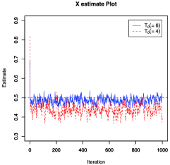
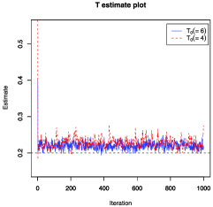
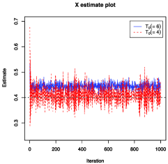
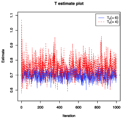
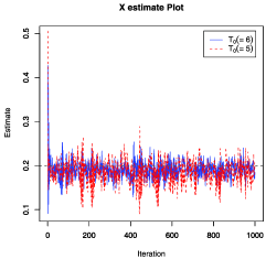
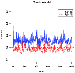
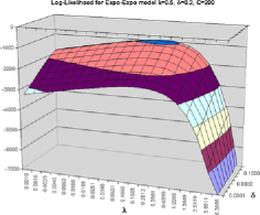
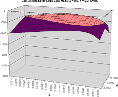
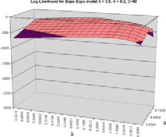
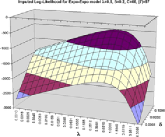
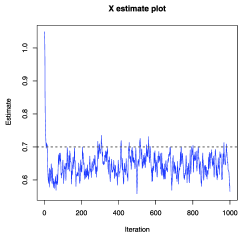
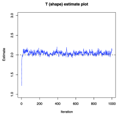
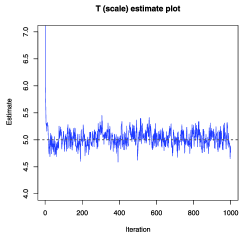
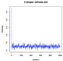
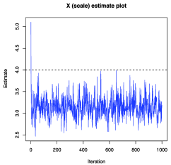
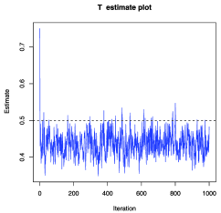
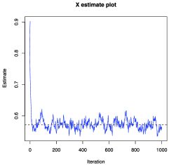
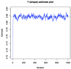
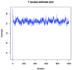
Table 1 represents the simulation results for different choices of distributions for $X$ and $T$. We choose $N=200$ for all experiments. We run the iteration $1000$ times for each model, of which we discard the first $100$ as burn-in values. The reported parameter estimates and standard deviations are based on the remaining $900$ iterations. We also report the convergence iteration number, which, for the multi-parameter case, represents the maximum of all iterations taken by individual parameters to satisfy $|\frac{\mu_{i+p}-\mu_{i}}{\mu_{i+p}}|<\varepsilon$. As we can see from Table 1, convergence is achieved quickly. For parameter estimation we used the maximum likelihood approach which is described briefly in the Appendix section. Again for other nontrivial distributions with complicated MLE, the method of moments or rank regression based approaches [Johnson (1964)] could be used. In each model, following standard practice, we obtain the initial parameter estimates for the distribution of $X$ and $T$ using the right truncated distribution. These initial estimates are way off in all cases, which explains why standard practice is unsatisfactory in this nontrivial situation. We summarize our simulation result in Table 1. The first two rows in Table 1 are of special interest since we assumed $X,T\stackrel{{\scriptstyle\mathrm{i.i.d.}}}{{\sim}}\operatorname{Exp}(\lambda=\delta)$. As shown in Appendix B.5, the exact likelihood given in equation (2) can be solved numerically in this case. For $T_{0}=6$ the exact likelihood based MLE yields $\widehat{\lambda}=0.22$ with asymptotic standard deviation $\widehat{\sigma}_{\lambda}=0.026$. For $T_{0}=5$, we get $\widehat{\lambda}=0.18$ with asymptotic standard deviation $\widehat{\sigma}_{\lambda}=0.028$. In both of these cases our simulation result is very close to the true value ($\lambda=\delta=0.2$) even though we did not use the information that $\lambda=\delta$ in our proposed algorithm. In Figure 4 we present pictorially the result for these two cases. This supports the viability of our algorithm. Next we explore non-i.i.d. cases. Figure 3 presents the case for $X\sim\operatorname{Exp}(\lambda)$ and $T\sim\operatorname{Exp}(\delta)$ with two different observation times ($T_{0}=4,6$). In the first case, we choose the true model parameters in such a way that about $50\%$ of the cases are observed (i.e., $C>100$). Figure 3(a) and (b) present the case when $\lambda=0.5$ and $\delta=0.2$. We observe $108$ and $66$ units for $T_{0}=6$ and $4$, respectively. As expected, the case with more units produces better estimates. Nevertheless, we point out that for $T_{0}=4$, even though we observe only about $33\%$ of the units, the final parameter estimates are still noticeably close to the true parameter values. Similar observations could be made for the other choice of parameter values in Figure 3(c) and (d). To elucidate the problem when using the exact maximum likelihood based approach, we have also plotted the log-likelihood surface (obtained via equation (2) and numerical integration) in Figure 5 for the case $\lambda=0.5$ and $\delta=0.2$. Figure 5(a) represents the case when we have complete observations for all units ($C=N$). However, as $T_{0}$ shrinks, $C$ goes down, and, as a result, the likelihood surface becomes very flat. Hence, searching for the MLE becomes computationally challenging and often leads to large variance. We have noted this problem earlier in Section 2. Figure 5(d) presents the log-likelihood surface obtained via equation (6) when imputation is in use. This representative plot is obtained for a specific iteration when $97$ units are imputed while running the algorithm described in Section 5. The flatness of the resulting log-likelihood surfaces in Figure 5(c) and (d) is an indicator of computational difficulties in finding the MLE for each case. Next, in Figure 6 we describe the iteration result when $X\sim\operatorname{Exp}(\lambda)$ and $T\sim\operatorname{Weibull}(\beta,\theta)$. In Figure 7 we describe the iteration result when $X\sim\operatorname{Weibull}(\beta,\theta)$ and $T\sim\operatorname{Exp}(\lambda)$. In all cases the final estimates are quite close to the true model parameters. Though not reported here, we obtain similar results with the gamma distribution. For details of the sampling from a truncated gamma distribution, please refer to Damien and Walker (2001). We have confined our simulation exploration only to commonly used reliability distributions; however, we are hopeful that the algorithm presented here will also work for other distributions with nonnegative support.

(a)	(b)

(c)

Figure 6: Plot of the maximum likelihood estimate for the Exponential–Weibull model over different iterations. The “$\cdots$” (dashed line) indicates true value of the parameter in each case.

(a)	(b)

(c)

Figure 7: Plot of the maximum likelihood estimate for the Weibull–Exponential model over different iterations. The “$\cdots$” (dashed line) indicates true value of the parameter in each case.

(a)	(b)
(c)	(d)

Figure 8: Plot (a) represents violin plot for the observed 133 units. Other plots represent the maximum likelihood estimates for the Furnace data over different iterations. The “$\cdots$” (dashed line) indicates finally estimated mean of the parameter in each case.

8 Motivating application.

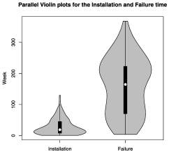
The data set that we will analyze using the current procedure came from an industrial house producing residential furnace components during one week in May $2001$. We consider a batch with $N=400$ units. The data consist of $C=133$ pairs of points as observed units (i.e., $\{x_{i},t_{i}\}_{i=1}^{133}$), which have failed within the observation time of seven years from the date of manufacturing. Figure 8(a) shows a violin plot for installation and failure times. The violin plot is a combination of a box plot and a kernel density plot. There is no specific information available about the remaining units. We are assuming that there exists no unit which has failed but was not reported. In practice, this could have happened for many other reasons. In the present context the reliability engineers believe that it is appropriate to model installation time ($X$) using an exponential distribution, while failure time ($T$) is modeled according to a Weibull distribution [Jager and Bertsche (2004); Zhu (2007)]. It should be noted that seasonality plays an important role in selling, installation and duty cycles (how rigorously the unit is being used) of the product. However, since in the present case we consider only a single batch, we assume that these effects will be similar for every unit in the batch. When comparing the units produced under different batches (and possibly produced at different times of the year), additional care is required as the independence assumption between $X$ and $T$ becomes questionable. This is due to the fact that some installation times are associated with severe duty cycles and more reliability problems.

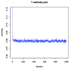
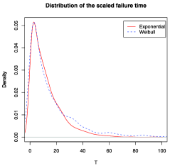
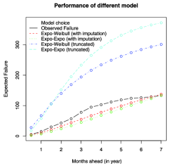
Before running the algorithm we divide the installation times as well as failure times by their corresponding standard deviation estimated from $133$ samples. This rescaling is done for numerical stabilization only, which results in faster convergence of the algorithm. Rescaled random variables have straightforward relationships with the original variables, without any drastic change to the distributional form. We run the algorithm for $1000$ iterations, however, convergence (with $p=5$, $\varepsilon=0.0005$) was achieved much earlier. We discard the first $100$ iterations as burn-in and report the estimates on the basis of the remaining $900$ iterations in Table 2. For model comparison purposes we have also investigated separately the case where $T$ is assumed to follow the exponential distribution, without altering the distribution of $X$. In each case we obtain the initial parameter estimates using the right truncated distributions. Figure 8 represents the case for the Exponential–Weibull model combination. Though the Exponential–Exponential model parameter is different from the previous choice (see Table 2), the density plot of the two distributions of $T$ are quite similar as depicted in Figure 9(b). We have also compared the predictive performance of different models in Figure 9(c), including the usual practice of truncated distributions without any imputation. We estimated the expected number of failures to be observed for different observation times over an interval of six months. This expected failure number is then compared with the observed failure number for the current data set. This required repeated re-estimation of model parameters at different time points. As can be seen, the truncated models have a huge overestimation problem throughout the study period. This again justifies our earlier criticism of current practice. Imputed models produce stable estimates and do much better even at the very early stage of product lifetime with only limited data. The Exponential–Weibull model choice does a little better than the Exponential–Exponential model. However, they are very much comparable as expected from Figure 9(b). It is desirable to estimate the expected failure number accurately for two main reasons. First, by accurately estimating warranty claims, an estimate of required financial reserves can be performed. This has immense implications in terms of future financial resource management. Second, it is desired to continuously improve the quality of consumer products, especially at the very high quality levels enjoyed by many consumer products today. All these aspects necessarily depend upon the accurate and efficient estimation of the reliability parameters (in $X$ and $T$). The method described in this paper provides a first step in this direction.

Table 2: Estimates for $N=400$ units in a single batch. $C=133$ units have complete observations

	Initial	Simulation	Average No.	Convergence	Time in
Distribution	estimate	result	imputations	iteration	second
$X\sim\operatorname{Exp}(\lambda)$	$\lambda=0.9$	$\widehat{\lambda}=0.57$, $\widehat{\sigma}_{\lambda}=0.014$	$260$	$167$	381
$T\sim\operatorname{Weibull}(\beta,\theta)$	$\beta=0.6$,	$\widehat{\beta}=0.81$, $\widehat{\sigma}_{\beta}=0.004$
	$\theta=3.18$	$\widehat{\theta}=14.47$, $\widehat{\sigma}_{\theta}=0.4$
$T\sim\operatorname{Exp}(\delta)$	$\delta=0.51$	$\widehat{\delta}=0.079$, $\widehat{\sigma}_{\delta}=0.001$	$263$	045	421

(a)	(b)

(c)

Figure 9: On the left, (a), maximum likelihood estimate for the furnace data when $T\sim\mathit{Exponential}$ distribution. In the middle, (b), density plot for two different model choices for $T$. Both look similar. On the right, (c), it represents performance of different models compared with the observed failure. Truncated distribution with no imputation performs very poorly with huge overestimation. Performance of imputed models are far better and the Exponential–Weibull model choice does the best job.

9 Concluding remarks.

Unlike electronic commodities, item specific tracking is not a feasible solution for many large scale industrial operations. Hence, the availability of both “complete” and “partial” information is quite common. In addition, except for very rare occasions, there are hardly any situations where all units in a batch start working at the same time. Unavailability of the installation time in a timely fashion is a major challenge to reliability engineers. Because of confidentiality issues we can not reveal any company specific information. However, we would like to mention that the above problem exists in different industrial sectors, and there is no clear solution thus far. In this paper we have proposed a computational approach to solve the problem with the optimal usage of partial and complete information. From a reliability engineer’s perspective, this current approach is simple, fast and also has straightforward interpretability.

The primary focus of any reliability analysis is the failure time. However, the waiting time for the installation is also very important in the sense that it provides valuable market specific information from the sales perspective, including seasonality and periodic sales patterns. In our approach we have targeted simultaneous estimation for both installation and failure time parameters in a combined fashion. To the best of our knowledge, this is the first attempt to do so. Finally, we would like to point out some of the assumptions that we have made in this paper, a violation of which will require more research. First, we have assumed that installation time and failure time are independent. This may be questionable in some situations as discussed in Section 8. Second, there is no aging effect for the units installed at different time points. Finally, we made the assumption that the distributional form of both installation and failure times is known. While for most of the legacy industrial products, in-house experts have a good idea about this from historical knowledge, it is of theoretical interest to see the effect of convergence and the quality of parameter estimates under incorrect parametric model specification. One way to avoid this is to choose a larger class of models. From the reliability perspective there is considerable effort to generalize Weibull and other popular reliability distributions [see Bali (2003) and Shao (2004)]. However, the resultant estimation procedure will be more involved. Another possibility is a nonparametric extension; however, the resulting procedure will be much more complex. In an ongoing work we are also exploring the exact probabilistic and inferential procedure based on equation (2).

Appendix A Proof of Theorem 3.2.

We can use the inequality (3.1) to argue that the following holds:

$$S_{T}(T_{0}-x_{k}) \leq P[T>T_{0}-X|x_{k}<X<x_{k+1}]\leq S_{T}(T_{0}-x_{k+1}),$$

$$S_{T}(T_{0}-x_{k-1}) \leq P[T>T_{0}-X|x_{k-1}<X<x_{k}]\leq S_{T}(T_{0}-x_{k}).$$

Combining both of these yields the proof.

Appendix B Maximum likelihood estimation.

We concentrate here on Exponential and Weibull distribution as used in the simulation, though other distributions with positive support, such as gamma and log-normal, can also be considered. Most of the results are published elsewhere and referenced as required.

B.1 Truncated exponential.

Let $X\sim\operatorname{Exp}(\lambda)$ with $0\leq X\leq T_{0}$. The p.d.f. is given by

$$f(x|\lambda,T_{0})=\frac{\lambda\exp(-x\lambda)}{1-\exp{(-T_{0}\lambda)}}.$$

If we have $n$ observations, then differentiating the log-likelihood equation with respect to $\lambda$ and equating it to zero yields

$$\frac{1}{\lambda}-\frac{T_{0}\exp{(-T_{0}\lambda)}}{1-\exp{(-T_{0}\lambda)}}-\overline{x}=0.$$

The above equation needs to be solved numerically to get the MLE of $\lambda$.

B.2 Randomly right censored exponential.

Let $T\sim\operatorname{Exp}(\lambda)$ and we observe $T^{\ast}=\min\{T,C_{r}\}$, where in the current context $C_{r}=T_{0}-X$ and $X$ is another random variable denoting installation time. Let us denote our samples as $\{t_{i}^{\ast},\delta_{i}\}_{i=1}^{n}$, where $\delta_{i}=1$ means the sample is an actual observation and $0$ means it is censored. If we have $\sum_{i=1}^{n}\delta_{i}=C$ true observations, then the log-likelihood is given by

$$L(\lambda)=c\log\lambda-\lambda\sum_{i=1}^{C}t_{i}-\lambda\sum_{j=1}^{n-C}(T_{0}-x_{j}),$$

which upon equating to $0$ yields $\widehat{\lambda}=\frac{C}{\sum_{i=1}^{C}t_{i}+\sum_{j=1}^{n-C}(T_{0}-x_{j})}$.

B.3 Truncated Weibull.

The MLE calculation for the truncated Weibull distribution is somewhat involved and may not always exist. Some explicit mathematical formulations with the required regularity conditions are described in Mittal and Dahiya (1989). We briefly mention only the final result here that has been used in this paper. Suppose $X\sim\operatorname{Weibull}(\beta,\theta)$, but with $0\leq X\leq T_{0}$. Let us denote by $Y=\frac{X}{T_{0}}$. Unfortunately, the MLE for $\beta$ is not available in closed form and needs to be solved numerically using the equation

$$\frac{\sum_{i=1}^{n}y_{i}^{\beta}}{n}-\frac{\sum_{i=1}^{n}y_{i}^{\beta}\log y_{i}}{{n}/{\beta}+\sum_{i=1}^{n}\log y_{i}}+\biggl{[}\exp\biggl{\{}\frac{{n}/{\beta}+\sum_{i=1}^{n}\log y_{i}}{\sum_{i=1}^{n}y_{i}^{\beta}\log y_{i}}\biggr{\}}-1\biggr{]}^{-1}=0.$$

Once we know $\widehat{\beta}$, the MLE of $\theta$ is

$$\widehat{\theta}=T_{0}\biggl{(}\frac{\sum_{i=1}^{n}y_{i}^{\widehat{\beta}}\log y_{i}}{{n}/{\widehat{\beta}}+\sum_{i=1}^{n}\log y_{i}}\biggr{)}^{{1}/{\widehat{\beta}}}.$$

B.4 Randomly right censored Weibull.

Suppose $T\sim\operatorname{Weibull}(\beta,\theta)$. Similar to the randomly right censored exponential case $T^{\ast}=\min\{T,C_{r}\}$, where in the current context $C_{r}=T_{0}-X$. We denote our data set as $\{t_{i}^{\ast},\delta_{i}\}_{i=1}^{n}$ and $\sum_{i=1}^{n}\delta_{i}=C$. The MLE is given explicitly in Shao (2004) and Lemon (1975), which again needs to be solved numerically for $\beta$ using the equation

$$\frac{1}{{\beta}}+\frac{\sum_{i=1}^{n}\delta_{i}\operatorname{log}t_{i}^{\ast}}{C}-\frac{\sum_{i=1}^{n}(t_{i}^{\ast})^{{\beta}}\log t_{i}^{\ast}}{\sum_{i=1}^{n}(t_{i}^{\ast})^{{\beta}}}=0.$$

Once we know $\widehat{\beta}$, the MLE of $\theta$ is

$$\widehat{\theta}=\biggl{(}\frac{\sum_{i=1}^{n}(t_{i}^{\ast})^{\widehat{\beta}}}{C}\biggr{)}^{{1}/{\widehat{\beta}}}.$$

B.5 Derivation of the exact MLE for i.i.d. exponential case.

We assume $X,T\stackrel{{\scriptstyle\mathrm{i.i.d.}}}{{\sim}}\operatorname{Exp}(\lambda)$. The complete likelihood is given by

$$L(\lambda)\propto(\lambda)^{2C}e^{-\lambda\sum_{i=1}^{C}(x_{i}+t_{i})}[e^{-\lambda T_{0}}+T_{0}\lambda e^{-\lambda T_{0}}]^{N-C}.$$

Now differentiating the log-likelihood equation with respect to $\lambda$ and equating it to zero yields

$$\frac{2C}{\lambda}+\frac{T_{0}(N-C)}{1+\lambda T_{0}}-\sum_{i=1}^{C}(x_{i}+t_{i})-(N-C)T_{0}=0.$$

The equation needs to be solved numerically for $\lambda$ to obtain MLE.

References

- Abernethy (1996) Abernethy, R. B. (1996). The New Weibull Handbook, 2nd ed. Robert B. Abernethy, North Palm Beach, FL.
- Bali (2003) Bali, T. G. (2003). The generalized extreme value distribution. Econ. Lett. 79 423–427.
- Damien and Walker (2001) Damien, P. and Walker, G. (2001). Sampling truncated normal, beta and gamma distribution. J. Comput. Graph. Statist. 10 206–215. \MR1939697
- Ghosh (2009) Ghosh, S. (2009). Supplement to “An imputation-based approach for parameter estimation in the presence of ambiguous censoring with application in industrial supply chain.” DOI: 10.1214/10-AOAS348SUPP.
- Jager and Bertsche (2004) Jager, P. and Bertsche, B. (2004). A new approach to gathering failure behavior information about mechanical components based on expert knowledge. In Reliability and Maintainability Annual Symposium—RAMS 90–95. Los Angleles, CA.
- Johnson (1964) Johnson, L. G. (1964). The Statistical Treatment of Fatigue Experiments. Elsevier, Amsterdam.
- Kececioglu (1993) Kececioglu, D. B. (1993). Reliability and Life Testing Handbook 1. Prentice-Hall, Englewood Cliffs, NJ.
- Klein and Moeschberger (2005) Klein, J. P. and Moeschberger, M. L. (2005). Survival Analysis: Techniques for Censored and Truncated Data, 2nd ed. Springer, New York.
- Lemon (1975) Lemon, G. (1975). Maximum likelihood estimation for the three parameter Weibull distribution based on censored samples. Technometrics 17 247–254. \MR0365858
- Meeker and Escobar (1998) Meeker, W. Q. and Escobar, L. A. (1998). Statistical Methods for Reliability Data. Wiley, New York.
- Michael and Schucany (1986) Michael, J. R. and Schucany, W. R. (1986). Analysis of data from censored samples. In Goodness-of-Fit Techniques (R. B. D’Agostino and M. A. Stepehens, eds.). Marcel Dekker, New York.
- Mittal and Dahiya (1989) Mittal, M. M. and Dahiya, R. C. (1989). Estimating the parameters of a truncated Weibull distribution. Commun. Statist. 18 2027–2042. \MR1033111
- Shao (2004) Shao, Q. (2004). Notes on maximum likelihood estimation for the three parameter Burr XII distribution. Comput. Statist. Data Anal. 45 675–687. \MR2050262
- Wang (2004) Wang, W. (2004). Refined rank regression method with censors. Qual. Reliab. Eng. Int. 20 667–678.
- Zhu (2007) Zhu, X. (2007). Ultrasonic fatigue of E319 cast aluminum alloy in the long lifetime regime. Ph.D. thesis, Univ. Michigan.