What Phase of the Interstellar Medium Correlates with the Star Formation Rate?

Abstract

Nearby spiral galaxies show an extremely tight correlation between tracers of molecular hydrogen (H₂) in the interstellar medium (ISM) and tracers of recent star formation, but it is unclear whether this correlation is fundamental or accidental. In the galaxies that have been surveyed to date, H₂ resides predominantly in gravitationally bound clouds cooled by carbon monoxide (CO) molecules, but in galaxies of low metal content the correlations between bound clouds, CO, and H₂ break down, and it is unclear if the star formation rate will then correlate with H₂ or with some other quantity. Here we show that star formation will continue to follow H₂ independent of metallicity. This is not because H₂ is directly important for cooling, but instead because the transition from predominantly atomic hydrogen (H i) to H₂ occurs under the same conditions as a dramatic drop in gas temperature and Bonnor-Ebert mass that destabilizes clouds and initiates collapse. We use this model to compute how star formation rate will correlate with total gas mass, with mass of gas where the hydrogen is H₂, and with mass of gas where the carbon is CO in galaxies of varying metallicity, and show that preliminary observations match the trend we predict.

1. Introduction

Spiral galaxies near the Milky Way show strong correlation between the surface density of star formation and the surface density of molecular gas, but only a very weak correlation between star formation and the surface density of atomic gas (Kennicutt et al., 2007; Bigiel et al., 2008; Leroy et al., 2008). However, the origin of this behavior is highly debated. In many models for the star formation rate (Tan, 2000; Li et al., 2005; Silk & Norman, 2009; Dobbs & Pringle, 2009), the chemical state of the gas is assumed to be dynamically unimportant. In these models stars form wherever galactic-scale gravitational instabilities dictate that gas collects into gravitationally bound structures, without regard to whether those structures consist of atomic or molecular gas. The observed correlation between molecules and star formation occurs only because molecules form preferentially in the same bound structures where stars do.

In other models (Robertson & Kravtsov, 2008; Gnedin et al., 2009; Krumholz et al., 2009d; Pelupessy & Papadopoulos, 2009; Gnedin & Kravtsov, 2010; Fu et al., 2010), however, the underlying assumption is that star formation follows the chemical transition between atomic hydrogen (H i) and molecular hydrogen (H₂) as the dominant gas phase, or the transition from ionized carbon (C ii) to carbon monoxide (CO) as the primary coolant, independent of the global dynamics. Closely related to these are models in which the locations where stars can form is determined by the gas temperature, or by the interplay between gas temperature and gravitational stability (Elmegreen & Parravano, 1994; Schaye, 2004; Ostriker et al., 2010). It is not entirely clear how this is correlated with the chemical composition, although Schaye (2004) obtain the intriguing result, which anticipates to some extent the one we report here, that the formation of a cold phase is closely associated with the H i to H₂ transition. However, he did not consider how this relates to CO, the molecule usually observed in place of H₂.

All of these models produce similar results for nearby spiral galaxies, where the majority of gravitationally-bound structures are also molecular and cooled by CO. However, whether star formation follows global dynamics, the H i to H₂ transition, or the C ii to CO transition makes a very large difference for how star formation behaves in regions with substantially sub-Solar metal content, since the chemical states of the hydrogen and the carbon are sensitive to gas metallicity in different ways (van Dishoeck & Black, 1988; Krumholz et al., 2009c; Glover & Mac Low, 2010; Wolfire et al., 2010), while the prevalence of galactic-scale instabilities is very insensitive to metallicity. Moreover, any successful model must also be able to relate the star formation rate to observable quantities, which include H i and CO, but not (generally) the total mass of H₂.

At present observations possess limited power to discriminate between the models, although the limited data available for nearby low-metallicity dwarf galaxies such as the Small Magellanic Cloud hold out the promise of being able to distinguish whether metallicity affects star formation. However, the differences between the models have profound implications for our understanding of star formation in the high redshift universe, where average metallicities are much lower. For example, the difficulty of forming molecules in metal-poor gas has been proposed as an explanation for the observed (Wolfe & Chen, 2006; Wild et al., 2007) lack of star formation in damped Lyman $\alpha$ systems (Krumholz et al., 2009a; Gnedin & Kravtsov, 2010), but this explanation is only viable if transitions to molecular gas are necessary for star formation.

Here we investigate whether the chemical state of the gas is relevant for star formation by studying how the Bonnor-Ebert mass and the chemical state vary in spherical interstellar clouds of varying volume and column densities. We show that, for such clouds, the H i to H₂ transition is strongly associated with a dramatic drop in the temperature and Bonnor-Ebert mass within the cloud, across a very wide range of metallicities and environments. In Section 2 we describe our computation method, in Section 3 we report our results, and in Section 4 we discuss the implications of our results for observations. Finally, we summarize in Section 5.

2. Computation Method

To minimize clutter we summarize all the physical parameters that enter our model in Table 1, and we discuss these choices in Appendix A. We also show in that Appendix that our results are robust against changes in these parameters. In this section we limit ourselves to a discussion of our calculation method.

Table 1 Fiducial parameter choices

Parameter	Value	Meaning	Reference
$\kappa$	$0.01(T/10\mbox{ K})^{2}Z^{\prime}$ cm2 g-1	IR dust opacity	Lesaffre et al. (2005)
$\alpha_{\rm gd}$ (H2)	$3.2\times 10^{-34}Z^{\prime}$ erg cm3 K-3/2	Dust-gas heat exchange rate	Goldsmith (2001)
$\alpha_{\rm gd}$ (H i)	$1.0\times 10^{-33}Z^{\prime}$ erg cm3 K-3/2	Dust-gas heat exchange rate	Appendix A
$q_{\rm CR}$ (H2)	12.25 eV	Energy / CR ionization	Appendix A
$q_{\rm CR}$ (H i)	6.5 eV	Energy / CR ionization	Dalgarno & McCray (1972)
$\zeta$	$2\times 10^{-17}Z^{\prime}$ s-1	CR ionization rate	Appendix A
$T_{\rm rad}$	8 K	Ambient radiation temperature	Appendix A
$G_{0}^{\prime}$	1	UV radiation intensity	Appendix A
$X_{\rm CII}$, $X_{\rm CO}$	$1.6\times 10^{-4}Z^{\prime}$	C ii / CO abundance	Sofia et al. (2004)
$\sigma_{d}$	$1\times 10^{-21}Z^{\prime}$ cm-2	UV dust opacity per H nucleus	Appendix A
$A_{V}/N_{\rm H}$	$4.0\times 10^{-22}Z^{\prime}$ mag cm2	Visual extinction per H column	Appendix A
OPR	0.25	Ratio of ortho- to para-H2	Neufeld et al. (2006)
$\sigma$	2 km s-1	Cloud velocity dispersion	Krumholz & Thompson (2007)

Note. — References to Appendix A mean that parameter choices are discussed there.

2.1. Physical Model

Consider a spherical cloud of mean volume density $n_{\rm H}$ H nuclei cm^-3 and mean column density $N_{\rm H}$ H nuclei cm^-2, mixed with dust with an absorption cross section per H nucleus $\sigma_{d}$ to photons near 1000 Å. The mean absorption optical depth to UV photons is $\tau=N_{\rm H}\sigma_{d}$, and the corresponding mean visual extinction at optical wavelengths is $A_{V}$. The outer parts of the cloud are exposed to the ultraviolet interstellar radiation field (ISRF) of the galaxy, and this keeps the hydrogen and carbon in the outer parts of the cloud predominantly in the form of H i and C ii. If the column density is sufficiently large, dust and the small population of hydrogen molecules in the predominantly atomic layer will absorb the ISRF, allowing a transition from H i to H₂ and C ii to CO as the main repositories of hydrogen and carbon. We assume that the gas is neutral, and that there are very few ionizing photons present.

In a real interstellar cloud, even if the density were uniform, the temperature and chemical composition would not be. Surface layers exposed to direct UV radiation would be warmer than the shielded interior, and the hydrogen there would be primarily H i rather than H₂. Thus there is no single cloud temperature or chemical composition we can compute, and determining the full temperature and chemical profile even when the density profile is given in advance requires solving a photodissociation region model in which one both simultaneously determines temperature and the chemical state, including line radiative transfer throughout the cloud. While there are many examples of such models in the literature, they are too computationally expensive to allow a wide search of parameter space, and they still rely on arbitrarily chosen density distributions. Instead, our goal is to estimate a single characteristic temperature and for a cloud, coupled to a simple description of its chemistry. To this end we will describe clouds’ chemical composition with single numbers giving the mass fraction in a given chemical phase, and we will approximate the cloud interior as a uniform region of volume density $n_{\rm H}$ and mean column density $N_{\rm H}$, consisting of gas at temperature $T_{g}$ uniformly mixed with dust of temperature $T_{d}$. For the purposes of computing the temperature, we will take the chemical composition to be uniform, with the hydrogen all as H i or H₂, and the carbon all as C ii or CO, despite the fact that every H₂ cloud has an outer H i shell, and every CO cloud has an outer C ii shell.

2.2. Chemical State

To compute the H i to H₂ transition in our model cloud, we rely on the models of Krumholz et al. (2008, 2009c), and McKee & Krumholz (2010) (collectively the KMT model hereafter). In these models the fraction of the hydrogen mass in the H₂-dominated region is given by

$$f_{\rm H_{2}}\approx 1-\left(\frac{3}{4}\right)\frac{s}{1+0.25s}$$ (1)

where

$$s = \frac{\ln(1+0.6\chi+0.01\chi^{2})}{0.6\tau}$$ (2)

$$\chi = 71\frac{G_{0}^{\prime}}{n_{\rm H}/\mbox{cm}^{-3}}$$ (3)

and $G_{0}^{\prime}$ is the strength of the ISRF normalized to its value in the Solar vicinity (which corresponds to a free-space H₂ dissociation rate of $5.4\times 10^{-11}$ s^-1). Note that, unlike some of the other approximate expressions derived by KMT, this one applies independent of whether the gas is warm or cold neutral medium. It should also be noted that this model assumes chemical equilibrium, which is not necessarily the case for H₂ (Pelupessy & Papadopoulos, 2009; Mac Low & Glover, 2010). However, Krumholz & Gnedin (2011) perform a detailed comparison between the equilibrium approximation and a set of galaxy simulations including full time-dependent chemistry and radiation. They find that the approximation is very accurate at metallicities of $Z^{\prime}\gtrsim 0.01$, where $Z^{\prime}$ is the metallicity normalized to the Milky Way value, and we can therefore use it safely. We note that equation (1) also agrees extremely well with observations both of local galaxies (Krumholz et al., 2009c) and of damped Lyman $\alpha$ systems at high redshift (Krumholz et al., 2009b). We therefore conclude that, on the galactic scales relevant to this work (as opposed to the isolated periodic boxes considered by Mac Low & Glover 2010) this approximation is valid.

The C ii to CO transition is predominantly governed by dust extinction, and thus is sensitive primarily to the cloud optical depth. At high optical depths wherever the hydrogen is H₂ the carbon is also CO, while at low optical depths there can be significant regions of H₂ where the carbon is primarily C ii, because the H₂ self-shields while the CO cannot (Glover & Mac Low, 2010; Wolfire et al., 2010). Recent semi-analytic work indicates that the ratio of mass where the carbon is CO to total cloud mass is (Wolfire et al., 2010)

$$f_{\rm CO}=f_{\rm H_{2}}e^{-4.0\left(0.53-0.045\ln\frac{G_{0}^{\prime}}{n_{\rm H}/{\rm cm}^{-3}}-0.097\ln Z^{\prime}\right)/A_{V}}.$$ (4)

Alternately, an empirical fit to numerical simulations for the same quantity (Glover & Mac Low, 2010) gives very similar results.

2.3. Thermal State

The temperatures of gas and dust are set by the condition of thermal equilibrium, following a method that combines elements from Goldsmith (2001) and Lesaffre et al. (2005). We consider heating of the gas by the grain photoelectric effect at a rate per H nucleus $\Gamma_{\rm pe}$, heating by cosmic rays at a rate $\Gamma_{\rm cr}$, and cooling via atomic and molecular line emission at a rate $\Lambda_{\rm line}$. Dust is heated via an external radiation field at a rate $\Gamma_{\rm dust}$, and cools via thermal emission at a rate $\Lambda_{\rm dust}$. Finally, energy flows from the dust to the gas at a rate $\Psi_{\rm gd}$, which may be negative if the gas is hotter than the dust. The condition for thermal balance is therefore that the temperatures $T_{g}$ and $T_{d}$ simultaneously satisfy the equations

$$\Gamma_{\rm pe}+\Gamma_{\rm cr}-\Lambda_{\rm line}+\Psi_{\rm gd} = 0$$ (5)

$$\Gamma_{\rm dust}-\Lambda_{\rm dust}-\Psi_{\rm gd} = 0.$$ (6)

Note that we do not include photoionization heating. While this is important at low column densities (e.g. Schaye, 2004), the lowest column density clouds we will consider in this work have optical depths of $\sim 10^{3}$ to ionizing photons, and thus photoionization heating is unimportant for them except very close to their surfaces.

To solve this equation we must compute the temperature dependence of each heating and cooling term. We assume that the clouds in question are optically thin to far-infrared radiation, so we need not consider trapping of the dust radiation field. Thus the dust cooling rate is

$$\Lambda_{\rm dust}=\kappa(T_{d})\mu_{\rm H}caT_{d}^{4},$$ (7)

where $c$ is the speed of light, $a$ is the radiation constant, $\kappa(T_{d})$ is the temperature-dependent dust specific opacity and $\mu_{\rm H}$ is the mean mass per H nucleus. Dust heating is more complex, as mentioned above, since the external interstellar ultraviolet field dominates at cloud edges and the local re-radiated infrared field dominates at cloud centers. Since we are mostly interested in what happens when clouds are shielded by at least a few magnitudes of extinction in the ultraviolet, we choose to adopt the IR-dominated case. In practice this choice makes very little difference, since the dust gas coupling is a very minor effect at the densities where we focus our attention. We characterize the IR radiation field by an effective temperature $T_{\rm rad}$, so

$$\Gamma_{\rm dust}=\kappa(T_{\rm rad})\mu_{\rm H}caT_{\rm rad}^{4}.$$ (8)

Finally, for the dust-gas energy exchange term we adopt the approximate exchange rate (Goldsmith, 2001)

$$\Psi_{\rm gd}=\alpha_{\rm gd}n_{\rm H}T_{g}^{1/2}(T_{d}-T_{g}),$$ (9)

where $\alpha_{\rm gd}$ is a coupling constant.

For the gas, the cosmic ray heating rate is

$$\Gamma_{\rm cr}=\zeta q_{\rm CR}\mbox{ s}^{-1}$$ (10)

where $\zeta$ is the cosmic ray primary ionization rate and $q_{\rm CR}$ is the thermal energy increase per primary cosmic ray ionization. For grain photoelectric heating, we must choose a suitable mean heating rate, since extinction through the cloud causes the heating rate to drop substantially as we move toward the interior. For simplicity, and since we are concerned more with cloud interiors than surfaces, we consider the heating rate to be attenuated by half the mean extinction of the cloud. With this approximation, we have

$$\Gamma_{\rm pe}=4.0\times 10^{-26}G_{0}^{\prime}e^{-N_{\rm H}\sigma_{d}/2}\mbox{ erg s}^{-1},$$ (11)

where $\sigma_{d}$ is the dust cross section per H nucleus to the UV photons that dominate grain photoelectric heating.

The final term in the thermal balance equations (5) and (6) is $\Lambda_{\rm line}$, the line cooling rate. In each case we consider only a single coolant species: C ii or CO. This is a reasonable approximation because, at the low temperatures where star formation occurs, one of these two will dominate. To compute the cooling rate we must compute the populations of the various levels, and we do so following the method of Krumholz & Thompson (2007). Let $f_{i}$ be the fraction of a given species, C ii or CO, in the $i$th state, and let $E_{i}$ be the energy of that state. Transitions between states $i$ and $j$ occur due to spontaneous emission, at a rate given by the Einstein coefficient $A_{ij}$ (which is zero if $E_{i}\leq E_{j}$), and due to collisions with with rate coefficient $\gamma_{ij,\rm S}$, where $S$ is the species of the collision partner. Note that the collision rate coefficients depend on the gas temperature. We do not consider stimulated emission or absorption due to an external radiation field, since neither is significant for the cooling lines of C ii or CO.

In the escape probability formalism we approximate that each spontaneously emitted photon produced by an atom transiting from level $i$ to level $j$ has a probability $\beta_{ij}$ of escaping; photons that do not escape are re-absorbed on the spot within the cloud, yielding no net change in the level populations. With these definitions and approximations, in statistical equilibrium the level populations are given implicitly by

$$f_{i}\sum_{j}\left(\beta_{ij}A_{ij}+n_{\rm HI}\gamma_{ij,\rm HI}+n_{\rm He}\gamma_{ij,\rm He}\right.$$

$$\left.{}+n_{\rm p-H_{2}}\gamma_{ij,\rm p-H_{2}}+n_{\rm o-H_{2}}\gamma_{ij,\rm o-H_{2}}\right)=$$

$$\sum_{i}\left(\beta_{ij}A_{ij}+n_{\rm HI}\gamma_{ij,\rm HI}+n_{\rm He}\gamma_{ij,\rm He}\right.$$

$$\left.{}+n_{\rm p-H_{2}}\gamma_{ij,\rm p-H_{2}}+n_{\rm o-H_{2}}\gamma_{ij,\rm o-H_{2}}\right)f_{i},$$ (12)

where the sums run over all quantum states, and $n_{\rm HI}$, $n_{\rm p-H_{2}}$, $n_{\rm o-H_{2}}$, and $n_{\rm He}$ are the number densities of H i, para-H₂, ortho-H₂, and He, respectively. The left hand side of this equation represents the rate of transitions out of state $i$ to all other states $j$, while the right hand side represents the rate of transitions into state $i$ from all other states $j$. The escape probabilities themselves depend on the level population. If we let $X$ be the abundance of the species in question relative to H nuclei, and $\sigma$ be the one-dimensional gas velocity dispersion, then we have (Krumholz & Thompson, 2007)

$$\beta_{ij}\approx\frac{1}{1+0.5\tau_{ij}},$$ (13)

where

$$\tau_{ij}=\frac{g_{i}}{g_{j}}\frac{3A_{ij}\lambda_{ij}^{3}}{16(2\pi)^{3/2}\sigma}XN_{\rm H}f_{j}\left(1-\frac{f_{i}g_{j}}{f_{j}g_{i}}\right),$$ (14)

$g_{i}$ and $g_{j}$ are the statistical weights of levels $i$ and $j$, and $\lambda_{ij}$ is the wavelength of a photon associated with the transition from level $i$ to level $j$.

Equations (12) – (14) constitute a complete system of algebraic equations for the level populations $f_{i}$. Given the solution to these equations, the line cooling rate per H nucleus is then given by

$$\Lambda_{\rm line}=\sum_{i,j}\beta_{ij}A_{ij}f_{i}h\nu_{ij}/n_{\rm H},$$ (15)

where $\nu_{ij}$ is the frequency of a photon emitted in a transition from state $i$ to state $j$.

We have now written down a complete set of equations to determine the gas and radiation temperatures. To solve them we use a double-iteration method. We first select trial values of $T_{d}$ and $T_{g}$, and then we compute all the heating and cooling rates $\Gamma$, $\Lambda$, and $\Psi$. In order to compute $\Lambda_{\rm line}$, we must solve for the equilibrium level populations $f_{i}$ by solving equations (12) – (14). We do so by fixing $T_{g}$ (and thus all the collision rate coefficients) and applying a Broyden’s method (Press et al., 1992). Once we have determined $\Lambda_{\rm line}$, we check if the thermal balance equations (5) and (6) are satisfied to within a specified tolerance. If not, we iteratively update $T_{d}$ and $T_{g}$ using Newton’s method to update $T_{d}$ and $T_{g}$ until equations (5) and (6) are satisfied to the required tolerance.

3. Results

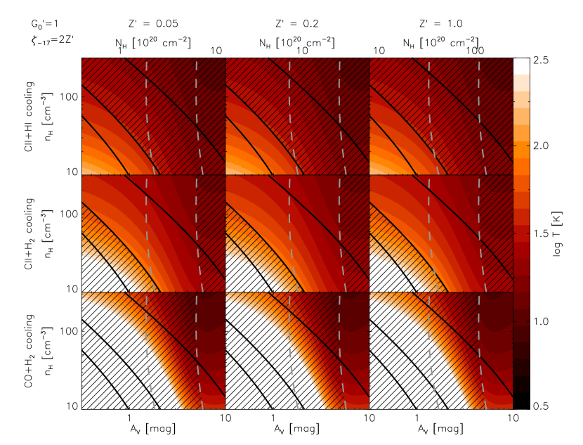
Figure 1.— Color indicates gas temperature as a function of density $n_{\rm H}$ and visual extinction $A_{V}$ for metallicities of $Z^{\prime}=0.05$, $0.2$, and $1.0$ (left to right columns; prime indicates relative to the Solar neighborhood value) and cooling by C ii plus H i (top row), C ii plus H₂ (middle row), and CO plus H₂ (bottom row) using our fiducial parameters $G_{0}^{\prime}=1$, $\zeta_{-17}=\zeta/10^{-17}\mbox{ s}^{-1}=2Z^{\prime}$ (upper left corner). Color contours run from $\log(T/\mbox{K})=0.5$ to $\log(T/\mbox{K})=2.5$ in steps of 0.1, with white representing $\log(T/\mbox{K})\geq 2.5$. The black solid lines are contours of $f_{\rm H_{2}}=0.1$, $0.5$, and $0.9$, from left to right. The gray dashed lines are contours of $f_{\rm CO}=0.1$ and $0.5$ from left to right; the $f_{\rm CO}=0.9$ contour lies off the plot to the right. Finally, the hatching pattern marks regions where the temperature and chemistry calculations are not fully consistent (e.g. because the chemistry calculation indicates that a cloud of that $A_{V}$ and $n$ should be dominated by H₂, but the temperature calculation assumes the hydrogen is H i).

We use the procedure outlined in Section 2 to compute the chemical state and temperature for a grid of clouds of varying $n_{\rm H}$ and $A_{V}$. Figure 1 shows the equilibrium temperature as a function of $n_{\rm H}$ and $A_{V}$, overlaid with contours of H₂ and CO fraction, computed for the three possible chemical compositions and gas metallicities of $Z^{\prime}=0.05$, $0.2$, and $1.0$. Recall that the chemical and thermal computations are decoupled, so the temperatures for C ii plus H i cooling should only be considered reliable to the left of $f_{\rm CO}=0.5$ and $f_{\rm H_{2}}=0.5$ contours, indicating the C ii to CO and H i to H₂ transitions, respectively. Similarly, the CO plus H₂ temperatures are only reliable to the right of both of these curves, while the C ii plus H₂ temperatures are reliable in the region between them.

Regardless of these limits on the regions of applicability, the striking result from these plots is that, independent of metallicity or chemical composition, there is a dramatic drop in temperature from hundreds of K to $\sim 10$ K as one moves from lower left (low density, low $A_{V}$) to upper right (high density, high $A_{V}$), and that the contours of constant temperature align remarkably well with contours of constant $f_{\rm H_{2}}$. This result is not surprising, because temperature and H₂ fraction depend on density and extinction in very similar ways. Both the heating and H₂ dissociation rate are proportional to the the exponential of minus the visual extinction, and both the cooling and H₂ formation rates are proportional to the square of the volume density. In contrast, contours of constant CO align much less well with temperature contours. The CO fraction depends primarily on $A_{V}$, with only a very weak density dependence. Furthermore, at $A_{V}$ high enough for the CO fraction to reach 50%, the grain photoelectric effect has been shut off so thoroughly that the temperature is insensitive to further increases in $A_{V}$.

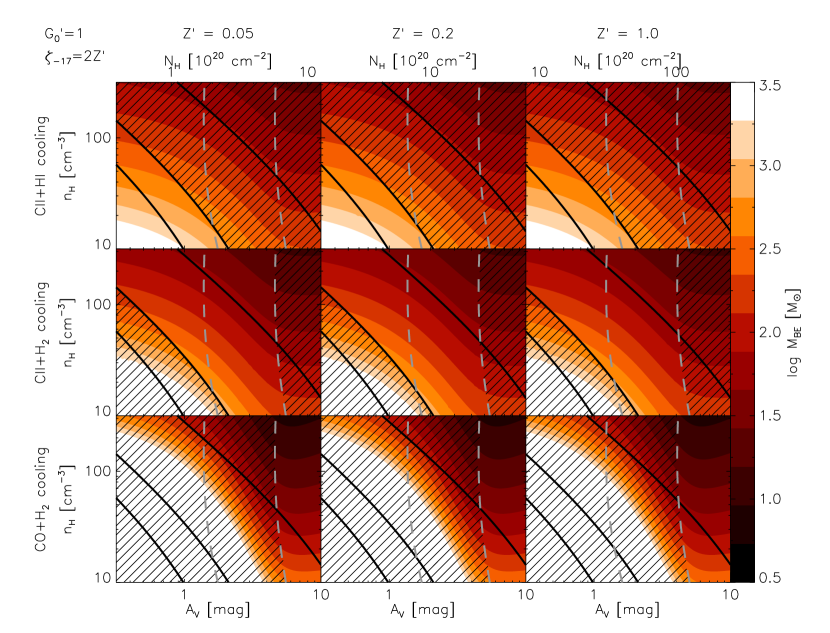
Figure 2.— Same as Figure 1, but with color indicating Bonnor-Ebert mass instead of temperature. Color contours run from $\log(M_{\rm BE}/M_{\odot})=0.5$ to $\log(M_{\rm BE}/M_{\odot})=3.5$ in steps of 0.25, with white representing $\log(M_{\rm BE}/M_{\odot})\geq 3.5$.

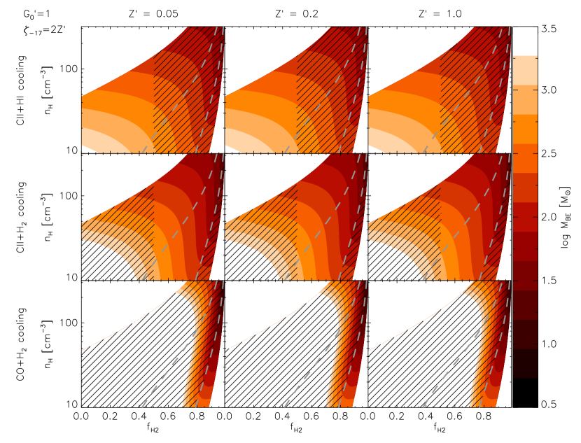
Figure 3.— Contours are the same as in Fig. 2, but the $x$ axis shows H₂ fraction rather than $A_{V}$. Note that not all of the grid is colored, because our grid in $n_{\rm H}$ and $A_{V}$ does not cover the full range in $n_{\rm H_{2}}$ and $f_{\rm H_{2}}$ shown.

Figures 2 and 3 show how the Bonnor-Ebert mass, the largest mass that can be supported against collapse by thermal pressure, changes with $A_{V}$ and with H₂ fraction as a result of this temperature change. This mass is

$$M_{\rm BE}=1.18\frac{c_{s}^{3}}{\sqrt{G^{3}n\mu_{\rm H}}}=1.18\left[\frac{(k_{B}T/\mu)^{3}}{G^{3}n\mu_{\rm H}}\right]^{1/2},$$ (16)

where $c_{s}$ is the isothermal sound speed, $T$ is the temperature, and $\mu_{\rm H}$ and $\mu$ are the mean mass per H nucleus and the mean particle mass, respectively. For Milky Way helium abundance, the former is $\mu_{\rm H}=2.3\times 10^{-24}$ g regardless of chemical composition, while the latter is $2.1\times 10^{-24}$ g for H i and $3.8\times 10^{-24}$ g for H₂. As the plot shows, there is a radical drop in the Bonnor-Ebert mass from thousands of $M_{\odot}$ to a few $M_{\odot}$ as one moves from low density and extinction to high density and extinction, and, as with the temperature, there is a very strong correlation between Bonnor-Ebert mass and H₂ fraction, while there is relatively little correlation with CO fraction. Figure 3 clearly shows that small Bonnor-Ebert masses are found exclusively in clouds with high H₂ fractions.

Our results imply that, in gas whose conditions are such that the hydrogen is mostly H i, structures with masses of $\sim 1000$ $M_{\odot}$ or less will be stabilized against collapse by thermal pressure. As a result, we conclude that star formation in such environments is extremely unlikely, in part because turbulence is extremely unlikely to generate fragments of such high masses that could then collapse (Padoan & Nordlund, 2002). Conversely, in gas where the hydrogen is mostly H₂, the mass that can be stabilized by thermal pressure is $2-3$ orders of magnitude smaller, turbulence generates numerous fragments capable of collapsing, and star formation is far more likely. It is important to note that the drop in Bonnor-Ebert mass and loss of stability is not caused by the H i to H₂ transition, it is simply very well correlated with it because the temperature and the H₂ fraction are determined by very similar combinations of extinction and density. We therefore conclude that star formation should correlate well with H₂, simply because H₂ is a good tracer of regions where thermal pressures are low enough to allow star formation.

4. Observational Consequences

4.1. Predictions for Observable Quantities

We can use our result that star formation correlates with H₂ to predict an approximate correlation between star formation rates and the masses of all gas, H₂ gas, and CO gas as a function of galaxy metallicity and surface density. Consider a portion of a galaxy with a mean surface density $\Sigma_{g}$ (averaged over the $\sim$kpc scales accessible to current observations). Within this region a fraction $f_{\rm H_{2}}$ of the gas, given by equation (1), is in the form of star-forming H₂ clouds, and within these a smaller fraction $f_{\rm CO}$ of the gas, given by equation (4), has most of its carbon in CO molecules.

We evaluate $f_{\rm H_{2}}$ following the methods outlined in Krumholz et al. (2009c, d). First, we must adopt a clumping factor $c$ to scale from the surface densities of individual atomic molecular complexes on $\sim 100$ pc scales to the $\sim$kpc scales accessible to current observations. This is necessary because the mean surface density averaged over a kpc-scale region that we observe is lower than the surface densities of the $\sim 100$ pc-sized giant molecular clouds, but it is the latter rather than the former that determines the atomic to molecular ratio in these clouds. Based on a combination of theoretical arguments and fits to observation, Krumholz et al. (2009c) adopt $c=5$, and we do so here, so $\tau=5\Sigma_{g}\sigma_{d}/\mu_{\rm H}$. Second, we adopt a characteristic value of $G_{0}^{\prime}/n=0.044(1+3.1Z^{\prime 0.365})/4.1$ expected for a two-phase atomic medium (Krumholz et al., 2009c, d). (For a given value of $G_{0}^{\prime}$, this corresponds to assuming that clouds on Figures 1 – 3 form a horizontal sequence at a fixed $n$ value that depends on $G_{0}^{\prime}$ and $Z^{\prime}$.) To evaluate $f_{\rm CO}$ and the star formation rate, we note that star-forming H₂ clouds appear to develop column densities $N_{\rm H}\sim 7.5\times 10^{21}$ cm^-2 ($\sim 85$ $M_{\odot}$ pc^-2) independent of galactic environment (Heyer et al., 2009; Bolatto et al., 2008; Krumholz et al., 2006). Since the CO-dominated regions are the inner parts of these clouds, this implies that the column density and $A_{V}$ that enter the calculation of the CO fraction should not be the mean galactic surface density or extinction, but instead the fixed $A_{V}$ of star-forming H₂ clouds. We adopt this value for $A_{V}$ in equation (4).

The corresponding star formation rate is expected on theoretical grounds to be approximately (Krumholz et al., 2009d)

$$\dot{\Sigma}_{*} = \frac{f_{\rm H_{2}}\Sigma_{g}}{2.6\mbox{ Gyr}}\times$$ (19)

$$\left\{\begin{array}[]{ll}(\Sigma_{g}/85\,M_{\odot}\,{\rm pc}^{-2})^{-0.33},&\Sigma_{g}<85\,M_{\odot}\,{\rm pc}^{-2}\\ (\Sigma_{g}/85\,M_{\odot}\,{\rm pc}^{-2})^{0.33},&\Sigma_{g}>85\,M_{\odot}\,{\rm pc}^{-2}\\ \end{array}\right..$$

In reality, based on the argument we have just made, we should compute the star formation rate not based directly on the H₂ fraction but instead based on the mass of cold gas. However, we have already seen that the H₂ and cold gas fractions are very similar, and equation (1) provides a convenient analytic approximation. We therefore use it to estimate both $f_{\rm H_{2}}$ and the star-forming gas fraction. We have therefore computed, for a portion of a galaxy of total gas surface density $\Sigma_{g}$ and metallicity $Z^{\prime}$, the expected surface densities of H₂, CO, and star formation.

Figure 4 shows our predicted correlation between specific star formation rate with respect to the mass of each gas constituent, $\mbox{SSFR}_{\rm(CO,H_{2},total)}=\dot{\Sigma}_{*}/\Sigma_{\rm(CO,H_{2},total)}$, and the surface density of that component at a range of metallicities. We see that at high surface densities and high metallicities the specific star formation rates for total gas, H₂, and CO are essentially identical, consistent with observations. At lower surface densities or metallicities, though, the star formation rate per unit total gas falls. Conversely, at lower metallicity the specific star formation with respect to CO rises, reflecting the fact that, at lower metallicity, the mass of gas where the chemical makeup is H₂ plus C ii rises as a fraction of the total H₂ mass. Since star formation follows H₂, $\mbox{SSFR}_{\rm CO}$ rises as a result. We note that Pelupessy & Papadopoulos (2009) reached a similar conclusion about $\mbox{SSFR}_{\rm CO}$ based on simulations that used a star formation recipe that assumed roughly constant $\mbox{SSFR}_{\rm H_{2}}$.

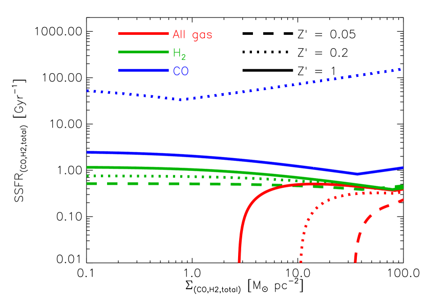
Figure 4.— Predicted gaseous specific star formation rate ${\rm SSFR}_{(\rm CO,H_{2},total)}=\dot{\Sigma}_{*}/\Sigma_{(\rm CO,H_{2},total)}=\dot{M}_{*}/M_{(\rm CO,H_{2},total)}$ as a function of gas surface density at fixed metallicity. The red lines indicate the specific star formation rate considering the total gas mass, green lines indicate the specific star formation rate for H₂, while blue lines indicate the specific star formation rate for gas where the carbon is CO rather than C ii. Dashed lines correspond to a metallicity $Z^{\prime}=0.05$, dotted lines to $Z^{\prime}=0.2$, and solid lines to $Z^{\prime}=1$. Note that the dashed blue line (${\rm SSFR}_{\rm CO}$ for $Z^{\prime}=0.05$) is above the range shown in the plot.

4.2. Comparison to Observations

The most striking feature of Figure 4 is that it predicts very strong variation in specific star formation rate with metallicity for CO and total gas, but not for H₂. In the low metallicity galaxies where we would like to test this prediction it is difficult to measure either the total gas mass or the H₂ mass, because we lack a reliable H₂ tracer except in a few limited cases (see Section 4.3 for further discussion). We can, however, measure CO luminosities and thereby estimate masses of gas that are CO-dominated. As shown in Figure 4, we predict that the specific star formation rate for CO should be much higher in the lower metallicity systems.

To test this prediction, we compile galaxy-integrated CO luminosities, $L_{\rm CO}$, and star formation rates, SFRs, from the literature. These measurements cover a wide range of metallicity from highly sub-Solar to super-Solar, and include both spirals and dwarfs. The data come from a variety of sources, summarized in Table 2. Whenever they are available, we give preference to $L_{\rm CO}$ derived from integrating complete single-dish maps of a galaxy, but many of the data still come from sparse sampling. For SFRs, we draw heavily from the recent set of galaxy-integrated measurements by Calzetti et al. (2010); these have the advantage of being computed in a uniform way and include an IR contribution to correct for extinction. Both $L_{\rm CO}$ and the SFR are luminosity-like quantities, so the ratio of the two is independent of distance. We also draw metallicities for each target from the literature. When available, we give preference to the recent compilation by Moustakas et al. (2010), using the average of their two characteristic metallicities. For targets not studied by Moustakas et al., we use values from the compilations by Marble et al. (2010), Calzetti et al. (2010), and Engelbracht et al. (2008) and a variety of literature sources.

Table 2Data compilation

Galaxy	$\log L_{\rm CO}$ [K km s${-1}$ pc2]	CO reference	$\log\dot{M}_{*}$ [$M_{\odot}$ yr${}^{-1}]$	SFR reference	$12+\log({\rm O}/{\rm H})$	Metallicity reference
SMC	$5.2\pm 0.2$	M06	$-1.3\pm 0.2$	W04	$8.0\pm 0.2$	D84; MA10
LMC	$6.5\pm 0.1$	F08	$-0.7\pm 0.2$	H09	$8.3\pm 0.3$	D84; MA10
IC10	$6.3\pm 0.2$	L06	$-1.0\pm 0.5$	L06	$8.2\pm 0.2$	L79; L03
M33	$7.6\pm 0.1$	H04	$0.0\pm 0.5$	H04	$8.3\pm 0.2$	R08
IIZw40	$6.2\pm 0.3$	T98	$-0.2\pm 0.3$	C10	$8.1\pm 0.3$	E08; C10
NGC1569	$5.1\pm 0.3$	T98	$-0.6\pm 0.3$	C10	$8.1\pm 0.2$	M97
NGC2537	$5.5\pm 0.3$	T98	$-1.1\pm 0.3$	C10	$8.4\pm 0.3$	MA10
NGC4449	$6.8\pm 0.3$	Y95	$-0.5\pm 0.3$	C10	$8.3\pm 0.2$	M97
NGC5253	$5.8\pm 0.3$	T98	$-0.3\pm 0.3$	C10	$8.2\pm 0.3$	MA10
NGC6822	$5.1\pm 0.2$	I97	$-2.0\pm 0.3$	C10	$8.4\pm 0.3$	MO10
NGC0628	$8.3\pm 0.1$	L09	$-0.2\pm 0.2$	C10	$8.8\pm 0.3$	MO10
NGC0925	$7.6\pm 0.1$	L09	$-0.3\pm 0.2$	C10	$8.6\pm 0.3$	MO10
NGC1482	$8.8\pm 0.3$	Y95	$0.5\pm 0.2$	C10	$8.6\pm 0.4$	MO10
NGC2146	$9.3\pm 0.3$	Y95	$0.9\pm 0.2$	C10	$8.7\pm 0.3$	E08; C10
NGC2403	$7.1\pm 0.3$	Y95	$-0.4\pm 0.2$	C10	$8.6\pm 0.2$	MO10
NGC2841	$8.4\pm 0.1$	L09	$0.1\pm 0.2$	C10	$9.0\pm 0.3$	MO10
NGC2782	$9.0\pm 0.3$	Y95	$0.7\pm 0.2$	C10	$8.6\pm 0.4$	E08; C10
NGC2798	$8.8\pm 0.3$	Y95	$0.5\pm 0.2$	C10	$8.7\pm 0.3$	MO10
NGC2976	$7.0\pm 0.1$	L09	$-1.0\pm 0.2$	C10	$8.7\pm 0.3$	MO10
NGC2903	$8.8\pm 0.1$	H03	$0.3\pm 0.2$	C10	$8.9\pm 0.3$	MA10
NGC3034	$8.8\pm 0.3$	Y95	$0.9\pm 0.2$	C10	$8.8\pm 0.3$	MO10
NGC3077	$6.0\pm 0.3$	T98	$-1.0\pm 0.2$	C10	$8.6\pm 0.3$	MA10
NGC3079	$9.4\pm 0.3$	Y95	$0.5\pm 0.2$	C10	$8.6\pm 0.4$	E08; C10
NGC3184	$8.4\pm 0.1$	L09	$-0.5\pm 0.2$	C10	$8.9\pm 0.3$	MO10
NGC3198	$7.9\pm 0.1$	L09	$-0.0\pm 0.2$	C10	$8.8\pm 0.3$	MO10
NGC3310	$8.2\pm 0.3$	Y95	$0.9\pm 0.2$	C10	$8.2\pm 0.4$	E08; C10
NGC3351	$8.2\pm 0.1$	L09	$-0.2\pm 0.2$	C10	$8.9\pm 0.3$	MO10
NGC3368	$8.3\pm 0.3$	Y95	$-0.4\pm 0.2$	C10	$9.0\pm 0.3$	MA10
NGC3521	$8.8\pm 0.1$	L09	$0.1\pm 0.2$	C10	$8.8\pm 0.3$	MO10
NGC3628	$9.2\pm 0.3$	Y95	$0.3\pm 0.2$	C10	$9.0\pm 0.3$	MA10
NGC3627	$9.0\pm 0.1$	H03	$0.2\pm 0.2$	C10	$8.7\pm 0.3$	MO10
NGC3938	$8.5\pm 0.1$	H03	$-0.1\pm 0.2$	C10	$8.7\pm 0.3$	E08; C10
NGC4194	$8.9\pm 0.3$	Y95	$1.1\pm 0.2$	C10	$8.7\pm 0.4$	E08; C10
NGC4214	$6.1\pm 0.1$	L09	$-1.0\pm 0.2$	C10	$8.2\pm 0.2$	T98
NGC4254	$9.9\pm 0.3$	Y95	$1.3\pm 0.2$	C10	$8.8\pm 0.3$	MO10
NGC4321	$9.2\pm 0.1$	H03	$0.4\pm 0.2$	C10	$8.8\pm 0.3$	MO10
NGC4450	$8.9\pm 0.3$	Y95	$-0.2\pm 0.2$	C10	$8.9\pm 0.4$	C10; MA10
NGC4536	$8.6\pm 0.3$	Y95	$0.3\pm 0.2$	C10	$8.6\pm 0.4$	MO10
NGC4569	$8.8\pm 0.1$	H03	$-0.1\pm 0.2$	C10	$8.9\pm 0.4$	E08; C10
NGC4579	$9.0\pm 0.3$	Y95	$0.2\pm 0.2$	C10	$9.0\pm 0.4$	C10; MA10
NGC4631	$8.5\pm 0.3$	Y95	$0.4\pm 0.2$	C10	$8.4\pm 0.3$	MO10
NGC4725	$9.1\pm 0.3$	Y95	$0.0\pm 0.2$	C10	$8.7\pm 0.4$	MO10
NGC4736	$7.9\pm 0.1$	L09	$-0.4\pm 0.2$	C10	$8.7\pm 0.4$	MO10
NGC4826	$8.1\pm 0.1$	H03	$-0.5\pm 0.2$	C10	$8.9\pm 0.3$	MO10
NGC5033	$9.3\pm 0.1$	H03	$0.1\pm 0.3$	K03	$8.7\pm 0.3$	MO10
NGC5055	$8.9\pm 0.1$	L09	$0.1\pm 0.2$	C10	$8.9\pm 0.4$	MO10
NGC5194	$9.2\pm 0.1$	H03	$0.4\pm 0.2$	C10	$9.0\pm 0.3$	MO10
NGC5236	$8.9\pm 0.1$	Y95	$0.4\pm 0.2$	C10	$9.0\pm 0.3$	MO10
NGC5713	$9.1\pm 0.3$	Y95	$0.6\pm 0.2$	C10	$8.7\pm 0.4$	MO10
NGC5866	$8.1\pm 0.3$	Y95	$-0.6\pm 0.2$	C10	$8.7\pm 0.4$	C10; MA10
NGC5953	$9.0\pm 0.3$	Y95	$0.4\pm 0.2$	C10	$8.7\pm 0.4$	E08; C10
NGC6946	$8.8\pm 0.1$	L09	$0.5\pm 0.2$	C10	$8.8\pm 0.3$	MO10
NGC7331	$9.0\pm 0.1$	L09	$0.4\pm 0.2$	C10	$8.8\pm 0.3$	MO10

Note. — C10 = Calzetti et al. (2010); D84 = Dufour (1984); E08 = Engelbracht et al. (2008); F08 = Fukui et al. (2008); H03 = Helfer et al. (2003); H04 = Heyer et al. (2004); H09 = Harris & Zaritsky (2009); I97 = Israel (1997); K03 = Kennicutt et al. (2003); L79 = Lequeux et al. (1979); L03 = Lee et al. (2003); L06 = Leroy et al. (2006); L09 = Leroy et al. (2009); M97 = Martin (1997); M06 = Mizuno et al. (2006); MA10 = Marble et al. (2010); MO10 = Moustakas et al. (2010) R08 = Rosolowsky & Simon (2008); T98 = Taylor et al. (1998); W04 = Wilke et al. (2004); Y95 = Young et al. (1995)

To convert observed CO $(1-0)$ luminosities to masses of gas traced by CO, we adopt a conversion factor $2\times 10^{20}$ H₂ molecules cm${}^{-2}/(\mbox{K km s}^{-1})^{-1}$ (Abdo et al., 2010b; Blitz et al., 2007; Draine et al., 2007; Heyer et al., 2009), so the mass is

$$M_{\rm CO}=4\times 10^{20}\mu_{\rm H}\left(\frac{L_{\rm CO}}{\mbox{K km s}^{-1}\mbox{ cm}^{2}}\right),$$ (20)

where $\mu_{\rm H}$ is the mean mass per H nucleus. This is equivalent to

$$\frac{M_{\rm CO}}{M_{\odot}}=\alpha_{\rm CO}\left(\frac{L_{\rm CO}}{\mbox{K km s}^{-1}\mbox{ pc}^{2}}\right)$$ (21)

with $\alpha_{\rm CO}=4.4$. Thus, we effectively assume a Milky Way conversion factor for CO-emitting gas. It is important to note that our $X$ factor represents the conversion from CO luminosity to mass of gas where the carbon is predominantly CO, and not the conversion from CO luminosity to total mass of gas where the hydrogen is H₂. These concepts are often not clearly distinguished in the literature. The approximately constant conversion factor derived from virial mass measurements of extragalactic clouds (Blitz et al., 2007; Bolatto et al., 2008) (which include some but not all of the H₂ that is not associated with CO) motivates this assumption, though there may still be changes in $\alpha_{\rm CO}$ of CO-emitting at the factor of 2 level across the range of metallicities that we study. The sense of these would be to increase $\alpha_{\rm CO}$, and to decrease the SFR-to-$M_{\rm CO}$ ratio, moving points down in Figure 5. Regardless of systematic effects, the y-axis in Figure 5 should be very close to the ratio of ionizing photon rate to CO luminosity.

To convert measured oxygen abundances to metallicities relative to Milky Way we adopt (Caffau et al., 2008)

$$\log Z^{\prime}=[12+\log({\rm O}/{\rm H})]-8.76.$$ (22)

As emphasized by Kewley & Ellison (2008) and Moustakas et al. (2010), the adopted calibration has a large influence on the metallicities derived from measurements of strong optical lines. Therefore the overall normalization of the metallicities in Figure 5 must be considered uncertain by at least $\sim 0.1-0.2$ dex, though the internal ordering is likely to be relatively robust.

A final complication is that most of the literature data we have gathered consists of galaxy-integrated values, rather than local values. We therefore do not have surface densities, and we must adopt characteristic values in order to compute the relationship between total gas, molecular gas, and CO luminosity. Fortunately, the results for the specific star formation rate for CO are not particularly sensitive to this assumption, as shown below.

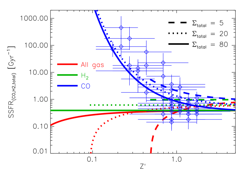
Figure 5.— Predicted gaseous specific star formation rate ${\rm SSFR}_{(\rm CO,H_{2},total)}=\dot{\Sigma}_{*}/\Sigma_{(\rm CO,H_{2},total)}=\dot{M}_{*}/M_{(\rm CO,H_{2},total)}$ as a function metallicity. As in Figure 4, the red lines indicate the specific star formation rate considering the total gas mass, green lines indicate the specific star formation rate for H₂, while blue lines indicate the specific star formation rate for gas where the carbon is CO rather than C ii. Dashed lines correspond to a total gas surface density $\Sigma_{\rm total}=5$ $M_{\odot}$ pc^-2, dotted lines to $\Sigma_{\rm total}=20$ $M_{\odot}$ pc^-2, and solid lines to $\Sigma_{\rm total}=80$ $M_{\odot}$ pc^-2. Note that these are all total gas surface densities, rather than surface densities of H₂ or CO as on the $x$ axis in Figure 4. Also note that we only show values for ${\rm SSFR}_{(\rm CO)}$ and ${\rm SSFR}_{(\rm H_{2})}$ for metallicities and surface densities that are high enough for$f_{\rm H_{2}}$ and $f_{\rm CO}$ to be non-zero.

We plot the literature data against our predictions in Figure 5. As the plot shows, there is a clear a correlation between SSFR_CO and metallicity that agrees within the uncertainties with what one expects if star formation follows H₂ rather than total gas or CO. Though the data are sparse with significant scatter, the difference appears to be more than 2 orders of magnitude in the SFR-to-CO ratio over about an order of magnitude in metallicity. The shape of this trend agrees well with our theoretical predictions. Given the uncertainties in estimating several of the parameters shown here, we believe this constitutes a reasonable first-check on the model. Future improvements to the measured dust-to-gas ratios, improved estimates of $\alpha_{\rm CO}$ from CO emitting gas, and observations of CO from larger samples of low-metallicity galaxies will improve the accuracy of the observed trend and allow more stringent tests.

The elevated value of SSFR_CO in dwarf galaxies and the outer parts of spirals relative to the inner parts of spirals has been pointed out before (Young et al., 1996; Leroy et al., 2006, 2007b; Gardan et al., 2007), but it was unclear if this was due to change in the star formation process or a change in the CO to H₂ ratio combined with star formation following H₂ rather than CO. Pelupessy & Papadopoulos (2009) argued that the elevated value of SSFR_CO could be explained if the latter were true, but they simply assumed that star formation was correlated with H₂, rather than explaining the correlation from first principles. Here we have provided the missing explanation, and Figure 5 demonstrates that a model based on it can quantitatively reproduce the observations.

4.3. Predictions for Future Observations

Figures 4 and 5 also contain clear predictions for observations. At present it is extremely difficult to measure either total gas masses or H₂ masses in galaxies with low metallicity, because CO breaks down as a tracer of H₂ in these environments, and because the H₂ itself does not emit. Observations are available for only a few galaxies based on using proxies other than CO for the H₂ (e.g. Leroy et al., 2007a). However, future dust observations with facilities such as Herschel and ALMA will make it easier to obtain H₂ masses, and thus total gas masses, for more galaxies. Our work contains a clear prediction: for these galaxies, the specific star formation rate with respect to H₂ mass should be essentially independent of metallicity, while the specific star formation rate for the total gas mass will behave in the opposite sense as for CO: low metallicity galaxies will have lower $\mbox{SSFR}_{\rm total}$, even as they have higher $\mbox{SSFR}_{\rm CO}$.

With resolved observations an additional test becomes possible. Figure 4 shows that $\mbox{SSFR}_{\rm total}$ is essentially flat at high surface densities, but turns down sharply at surface densities below a metallicity-dependent value. Such a drop is seen below $\Sigma_{\rm total}\lesssim 10$ $M_{\odot}$ pc^-2 in observations of Solar metallicity galaxies Bigiel et al. (2008). Models in which the star formation rate depends on global gravitational instability or similar phenomena that do not care about gas cooling or chemistry predict that the surface density at which the total gas specific star formation rate drops should not vary with metallicity (e.g. Li et al., 2006). In contrast, our work here suggests that it should scale roughly inversely with metallicity; Schaye (2004), using a thermally-based model that anticipates some of this work, makes a similar prediction (his equation 25), although the metallicity-dependence in his model is weaker than in ours. Resolved measurements of the total gas surface density in nearby galaxies should be able to test which prediction is correct: does $\mbox{SSFR}_{\rm total}$ always change sharply at $\sim 10$ $M_{\odot}$ pc^-2, or is that value metallicity-dependent? Preliminary results indicate appear consistent with a dependence on metallicity (Fumagalli et al., 2010), but a more systematic survey is needed.

5. Summary

In this paper we consider which phase of the interstellar medium should correlate best with the star formation rate, and why. Our work extends the previous examination of this problem by Schaye (2004). We use chemical and thermal models of interstellar clouds to show that the star formation rate is expected to correlate most closely with the molecular hydrogen content of a galaxy. In order to undergo runaway gravitational collapse to form stars, gas must be able to reach low temperatures and therefore low Bonnor-Ebert masses. Its ability to do so, however, is impaired by the interstellar radiation field, which heats the gas. Only in regions where the ISRF is sufficiently excluded by extinction can star formation occur. We find that such regions are also the regions where the gas is expected to be predominantly H₂ rather than H i, and for this reason the star formation rate correlates with, but is not caused by, the H i to H₂ transition. In contrast, the chemical makeup has relatively little effect on the ability of the gas to cool. All of these results are robust against a very wide range of variation in metallicity, radiation field, or other properties of the galactic environment.

That star formation correlates with H₂ rather than either total gas mass or CO mass has strong observational implications (see also Pelupessy & Papadopoulos, 2009). The fraction of H₂ gas where the carbon is in the form of C ii rather than CO is a strong function of metallicity. Galaxies with low metallicity tend to have large masses of H₂ where there is fairly little CO. If this material is able to form stars, as we predict, then the star formation rate per unit CO mass should be very large in low metallicity galaxies. We see that precisely this phenomenon is found in observed galaxies. Finally, we note that the fraction of the total gas mass where the hydrogen is H₂ rather than H i is also a strongly increasing function of metallicity. Since star formation correlates with H₂, we predict that the star formation rate per unit total gas mass should be small in low metallicity galaxies. This prediction can be used to test our calculations.

Appendix A Parameter Choices

All molecular and atomic information, including level energies, Einstein coefficients, and collision rate coefficients, is taken from the Leiden Atomic and Molecular Database (Schöier et al., 2005). Other input parameters are gathered from a variety of sources, and our fiducial values and references are given in Table 1. Most of these are straightforward, and where a quantity has been observed in the Milky Way, we extrapolate to other galaxies by assuming that element abundances and dust to gas ratios are simply proportional to metallicity. Parameters that are not directly observed or extrapolated we discuss in the remainder of this Appendix.

A.1. Dust-Gas Thermal Exchange Rate Coefficients

For the dust-gas thermal exchange rate coefficient $\alpha_{\rm dg}$, we adopt a standard value of $3.8\times 10^{-34}$ erg cm³ K^-3/2 in H₂-dominated gas in the Milky Way (Goldsmith, 2001), and we assume that this will also hold in galaxies of similar metallicity. We must extrapolate this both to lower metallicity galaxies, and to predominantly H i gas. For the former, we assume that the total surface area of grains is proportional to the metal abundance. For the latter, we must account for both the change in the number of particles and the masses of the individual particles, which alters their speed. We assume that the accommodation coefficient is equal for H, H₂, and He. (More accurate approximations are possible if the grain size distribution is known, e.g. Hollenbach & McKee (1979), but given the uncertainties in how size distributions vary from galaxy to galaxy and the relative lack of importance of this effect, we omit this complication.) With this assumption, the dust-gas energy exchange rate provided by gaseous members of species $X$ is proportional to $n_{X}/m_{X}^{1/2}$, where $n_{X}$ is the number density of members of that species and $m_{X}$ is the mass of that species. Thus in regions of atomic and molecular hydrogen respectively we have

$$\alpha_{\rm dg,HI} \propto \frac{n_{\rm HI}}{m_{\rm H}^{1/2}}+\frac{n_{\rm He}}{m_{\rm He}^{1/2}}$$ (A1)

$$\alpha_{\rm dg,H_{2}} \propto \frac{n_{\rm H_{2}}}{m_{\rm H_{2}}^{1/2}}+\frac{n_{\rm He}}{m_{\rm He}^{1/2}},$$ (A2)

where the constants of proportionality are the same in each case. In a predominantly atomic region $n_{\rm HI}=n_{\rm H}$, while in a predominantly molecular region $n_{\rm H_{2}}=n_{\rm H}/2$; in both cases $n_{\rm He}\approx n_{\rm H}/10$. Similarly, $m_{\rm He}=4m_{\rm H}$ and $m_{\rm H_{2}}=2m_{\rm H}$. Combining the dependence on metallicity with that on chemical phase, we arrive at our final expressions for $\alpha_{\rm dg}$:

$$\alpha_{\rm dg,H_{2}} = 3.8\times 10^{-33}Z^{\prime}\mbox{ erg cm}^{3}\mbox{ K}^{-3/2}$$ (A3)

$$\alpha_{\rm dg,HI} = 1.0\times 10^{-33}Z^{\prime}\mbox{ erg cm}^{3}\mbox{ K}^{-3/2}.$$ (A4)

For the radiation temperature, $T_{\rm rad}$, as discussed above we must select a single value to characterize the re-radiated infrared field within a cloud. We adopt $T_{\rm rad}=8$ K for this, near the minimum temperature seen in ammonia observations of Galactic cold clouds (Jijina et al., 1999). Both this choice and our choice of $\alpha_{\rm dg}$ have very little impact on our results due to the weak dust-gas coupling in the density range with which we are concerned.

A.2. Opacities

Our calculations depend on the absorption cross section per H nucleus $\sigma_{d}$ to UV photons, and the visual extinction per unit hydrogen column $A_{V}/N_{\rm H}$. Note that $\sigma_{d}$ reflects only absorption, while $A_{V}$ includes scattering as well. These quantities depend on the extinction curve and vary between dense and diffuse environments even within a single galaxy at a single metallicity, and thus their exact values are uncertain by a factor of two. As a guide we examine the values given by the models of Weingartner & Draine (2001) for the Milky Way, Large Magellanic Cloud, and Small Magellanic Cloud. Once we scale the LMC and SMC models to the same total dust to gas ratio as the Milky Way models, we obtain values of $\sigma_{d}/10^{-21}\mbox{ cm}^{-2}=0.7,1.7,2.0,1.8$ and $(A_{V}/N_{\rm H})/10^{-22}\mbox{ mag cm}^{-2}=4.5,5.1,3.6,2.8$ for Weingartner & Draine’s models for Milky Way sightlines with $R_{V}=5.5$, Milky Way sightlines with $R_{V}=3.1$, the average LMC sightline, and a sightline through the SMC bar, respectively. We therefore adopt intermediate values $\sigma_{d}=1.0\times 10^{-21}Z^{\prime}$ cm² and $A_{V}/N_{\rm H}=4.0\times 10^{-22}Z^{\prime}$ mag cm². With these fiducial choices, the UV absorption is larger than the the visual extinction by a factor of $2.5/1.08=2.31$ (where the factor of 1.08 accounts for the conversion from magnitudes to true dimensionless units).

A.3. Far Ultraviolet Radiation Field

The FUV radiation field, parameterized by $G_{0}^{\prime}$, affects both gas temperature and chemistry. There is no unique value of $G_{0}^{\prime}$ that characterizes all gas clouds across all galaxy types, and even within a single star-forming cloud the ambient UV field increases with time as stars form. As a fiducial choice we adopt $G_{0}^{\prime}=1$, the Solar neighborhood value. In regions where star formation is ongoing the mean is likely larger, but we are interested in the initiation of star formation, so it seems prudent to select a value typical of regions before the onset of star formation.

To test our sensitivity to this choice, we have recomputed our model grids with values of $G_{0}^{\prime}=0.1$ and $G_{0}^{\prime}=10$, and re-plotted Figures 1 – 3 of the main text in Figure 1. Not surprisingly, the H i to H₂, C ii to CO transitions, and warm to cold gas transitions all move to higher density and $A_{V}$ for higher $G_{0}^{\prime}$, and to lower density and $A_{V}$ for lower $G_{0}^{\prime}$. Nonetheless, over a factor of 100 range in $G_{0}^{\prime}$, we will retain the excellent correlation between the H i to H₂ transition and the drop in temperature from hundreds of K to $\sim 10$ K, along with the concomitant drop in the Bonnor-Ebert mass from several $1000$ $M_{\odot}$ or more to a few $M_{\odot}$. At all three values of $G_{0}^{\prime}$, contours of constant $f_{\rm H_{2}}$ align closely with contours of constant Bonnor-Ebert mass. In the lower two panels, note that, contours of constant $M_{\rm BE}$ remain largely vertical, indicating that the Bonnor-Ebert mass drops systematically as the H₂ fraction increases. Thus our conclusions are robust against large variations in $G_{0}^{\prime}$.

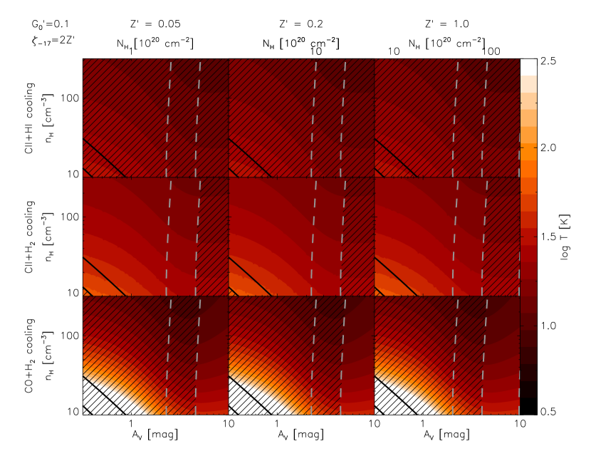
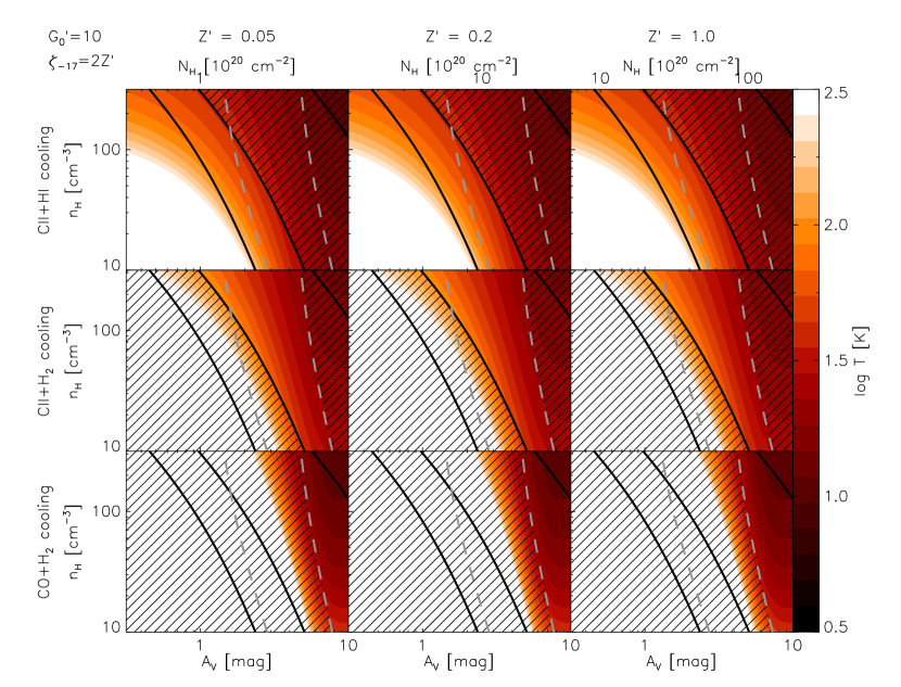
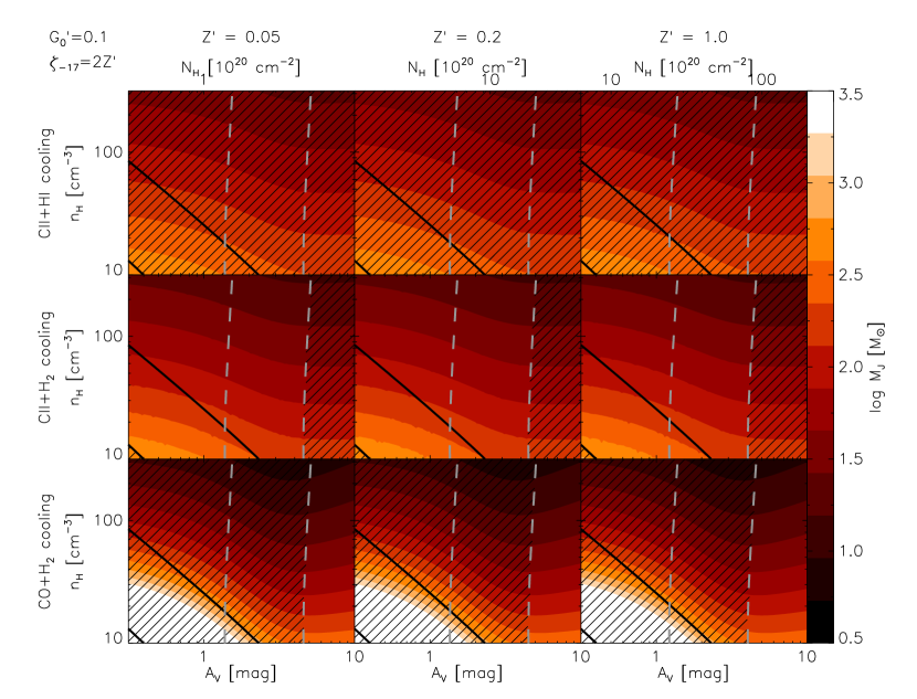
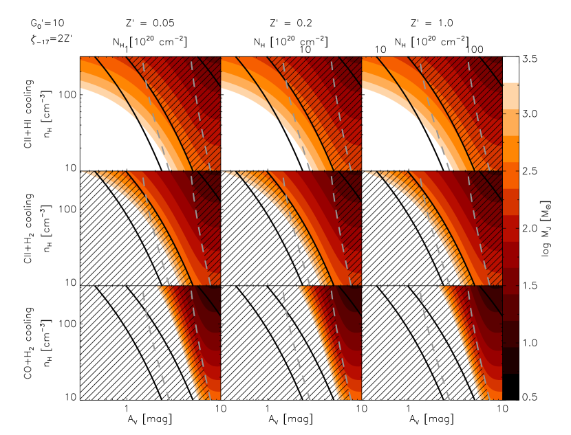
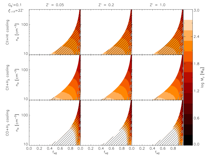
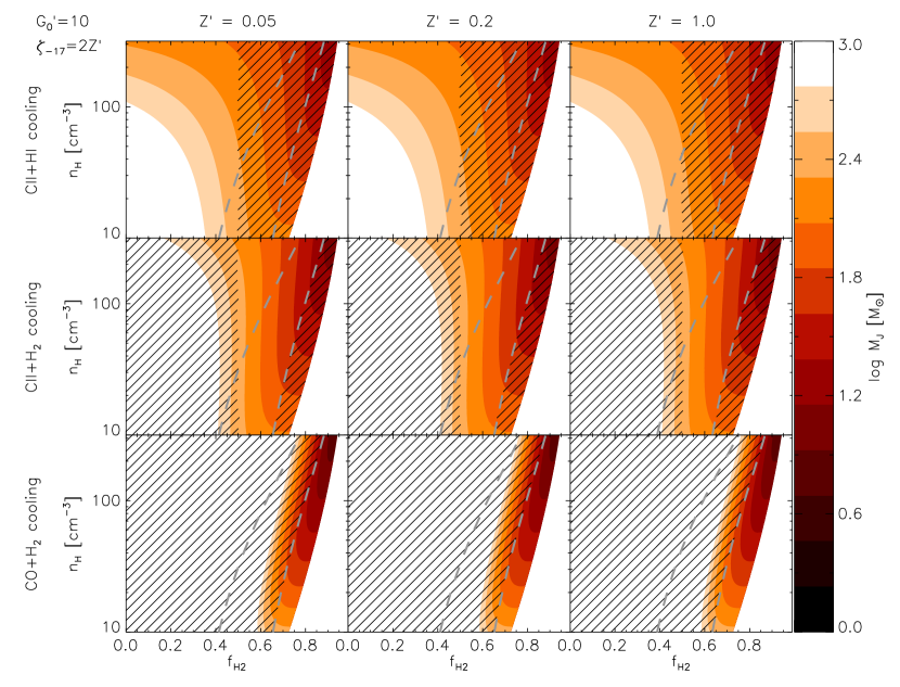
Figure 1.— Left column: same as Figures 1, 2, and 3, but with $G_{0}^{\prime}=0.1$ instead of $G_{0}^{\prime}=1$. Right column: same as Figures 1, 2, and 3, but with $G_{0}^{\prime}=10$ instead of $G_{0}^{\prime}=1$.

A.4. Cosmic Rays

The cosmic ray heating rate is uncertain in two ways. First, the energy yield per primary cosmic ray ionization $q_{\rm CR}$ is 6.5 eV in predominantly neutral H i (Dalgarno & McCray, 1972; Wolfire et al., 1995). In H₂ the yield is uncertain. Both dissociative recombination of H₂ and excitation of its rotational and vibrational levels followed by collisional de-excitation provide extra channels for energy transfer from primary cosmic ray electrons to thermal motion, but the importance of these processes is likely density-dependent. Values given in the literature range from nearly the same energy yield as in H i up to 20 eV per primary ionization (Glassgold & Langer, 1973; Dalgarno et al., 1999). We follow Wolfire et al. (2010) in adopting an intermediate value $q_{\rm CR}=12.25$ eV, but this should be regarded as uncertain by a factor of 2.

A similar uncertainty affects the cosmic ray ionization rate. For Milky Way-like galaxies we adopt $\zeta=2\times 10^{-17}$ s^-1 (Wolfire et al., 2010), but the primary cosmic ray ionization rate even in the Milky Way is substantially uncertain, and may be higher than this value (Neufeld et al., 2010). The cosmic ray intensity also varies with the star formation rate in galaxies (Abdo et al., 2010a). Thus in low metallicity galaxies, which also tend to have low star formation rates, the cosmic ray ionization rate is likely lower than the Milky Way value. The scaling is extremely uncertain; for lack of a better alternative, we simply take the cosmic ray ionization rate to scale with the metallicity.

To test our sensitivity to our choice of cosmic ray ionization rate, we have recomputed our temperature grid with cosmic ray ionization rates that are a factor of 3 larger and a factor of 3 smaller than our fiducial choice, thereby exploring a $\sim 1$ decade range in cosmic ray heating rate. We plot the results in Figure 2. Again, we see that the results are robust, in the sense that contours of constant Bonnor-Ebert mass remain closely aligned with contours of constant H₂ fraction as we vary the cosmic ray ionization rate.

We do caution, however, that this breaks down if we select a cosmic ray ionization rate that is extremely high (more than $10-30$ times our fiducial one). For such high cosmic ray ionization rates, cosmic ray heating becomes more important than grain photoelectric heating even in unshielded, low $A_{V}$ gas. In this case the temperature and Bonnor-Ebert mass become uncorrelated with $A_{V}$, and vary with density alone. However, such high cosmic ray ionization rates are inconsistent with observations in the Milky Way.

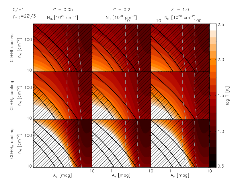
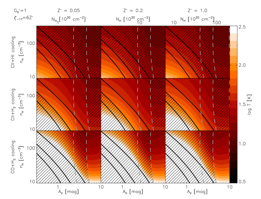
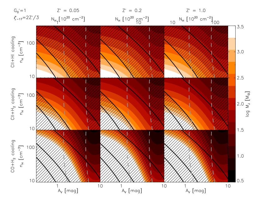
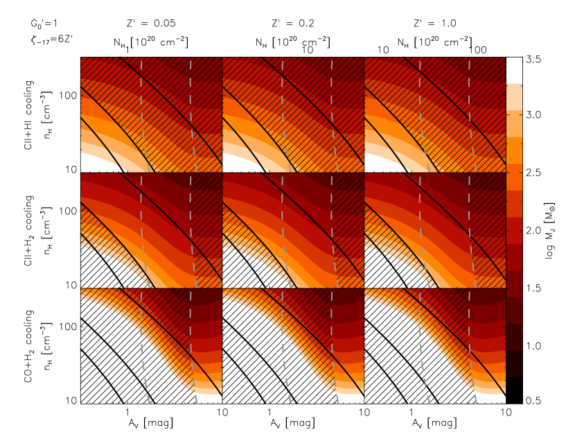
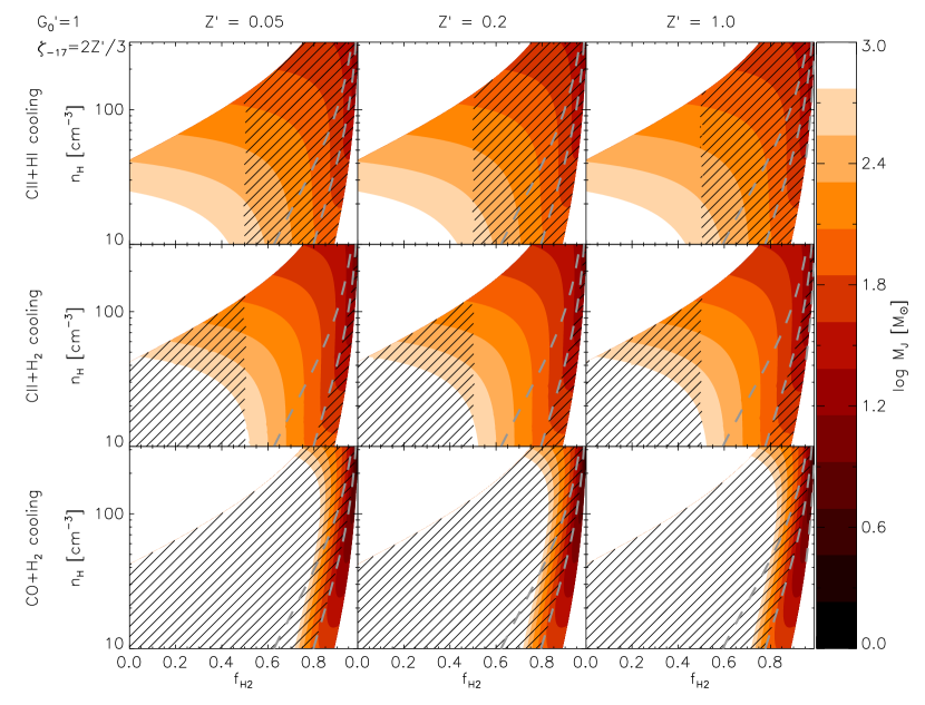
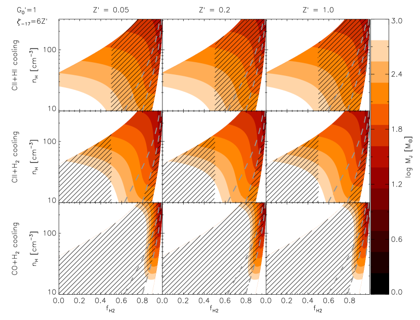
Figure 2.— Left column: same as Figures 1, 2, and 3, but with $\zeta=0.67\times 10^{-17}$ s^-1 instead of $\zeta=2\times 10^{-17}$ s^-1. Right column: same as Figures 1, 2, and 3, but with $\zeta=6\times 10^{-17}$ s^-1 instead of $\zeta=2\times 10^{-17}$ s^-1

References

- Abdo et al. (2010a) Abdo, A. A., et al. 2010a, ApJ, 709, L152
- Abdo et al. (2010b) —. 2010b, ApJ, 710, 133
- Bigiel et al. (2008) Bigiel, F., Leroy, A., Walter, F., Brinks, E., de Blok, W. J. G., Madore, B., & Thornley, M. D. 2008, AJ, 136, 2846
- Blitz et al. (2007) Blitz, L., Fukui, Y., Kawamura, A., Leroy, A., Mizuno, N., & Rosolowsky, E. 2007, in Protostars and Planets V, ed. B. Reipurth, D. Jewitt, & K. Keil, 81–96
- Bolatto et al. (2008) Bolatto, A. D., Leroy, A. K., Rosolowsky, E., Walter, F., & Blitz, L. 2008, ApJ, 686, 948
- Caffau et al. (2008) Caffau, E., Sbordone, L., Ludwig, H., Bonifacio, P., Steffen, M., & Behara, N. T. 2008, A&A, 483, 591
- Calzetti et al. (2010) Calzetti, D., et al. 2010, ApJ, 714, 1256
- Dalgarno & McCray (1972) Dalgarno, A., & McCray, R. A. 1972, ARA&A, 10, 375
- Dalgarno et al. (1999) Dalgarno, A., Yan, M., & Liu, W. 1999, ApJS, 125, 237
- Dobbs & Pringle (2009) Dobbs, C. L., & Pringle, J. E. 2009, MNRAS, 396, 1579
- Draine (2003) Draine, B. T. 2003, ARA&A, 41, 241
- Draine et al. (2007) Draine, B. T., et al. 2007, ApJ, 663, 866
- Dufour (1984) Dufour, R. J. 1984, in IAU Symposium, Vol. 108, Structure and Evolution of the Magellanic Clouds, ed. S. van den Bergh & K. S. D. Boer, 353–360
- Elmegreen & Parravano (1994) Elmegreen, B. G., & Parravano, A. 1994, ApJ, 435, L121+
- Engelbracht et al. (2008) Engelbracht, C. W., Rieke, G. H., Gordon, K. D., Smith, J., Werner, M. W., Moustakas, J., Willmer, C. N. A., & Vanzi, L. 2008, ApJ, 678, 804
- Fu et al. (2010) Fu, J., Guo, Q., Kauffmann, G., & Krumholz, M. R. 2010, MNRAS, 409, 515
- Fukui et al. (2008) Fukui, Y., et al. 2008, ApJS, 178, 56
- Fumagalli et al. (2010) Fumagalli, M., Krumholz, M. R., & Hunt, L. K. 2010, ApJ, 722, 919
- Gardan et al. (2007) Gardan, E., Braine, J., Schuster, K. F., Brouillet, N., & Sievers, A. 2007, A&A, 473, 91
- Glassgold & Langer (1973) Glassgold, A. E., & Langer, W. D. 1973, ApJ, 186, 859
- Glover & Mac Low (2010) Glover, S. C. O., & Mac Low, M. 2010, MNRAS, submitted, arXiv:1003.1340
- Gnedin & Kravtsov (2010) Gnedin, N. Y., & Kravtsov, A. V. 2010, ApJ, 714, 287
- Gnedin et al. (2009) Gnedin, N. Y., Tassis, K., & Kravtsov, A. V. 2009, ApJ, 697, 55
- Goldsmith (2001) Goldsmith, P. F. 2001, ApJ, 557, 736
- Harris & Zaritsky (2009) Harris, J., & Zaritsky, D. 2009, AJ, 138, 1243
- Helfer et al. (2003) Helfer, T. T., Thornley, M. D., Regan, M. W., Wong, T., Sheth, K., Vogel, S. N., Blitz, L., & Bock, D. C.-J. 2003, ApJS, 145, 259
- Heyer et al. (2009) Heyer, M., Krawczyk, C., Duval, J., & Jackson, J. M. 2009, ApJ, 699, 1092
- Heyer et al. (2004) Heyer, M. H., Corbelli, E., Schneider, S. E., & Young, J. S. 2004, ApJ, 602, 723
- Hollenbach & McKee (1979) Hollenbach, D., & McKee, C. F. 1979, ApJS, 41, 555
- Israel (1997) Israel, F. P. 1997, A&A, 328, 471
- Jijina et al. (1999) Jijina, J., Myers, P. C., & Adams, F. C. 1999, ApJS, 125, 161
- Kennicutt et al. (2003) Kennicutt, Jr., R. C., et al. 2003, PASP, 115, 928
- Kennicutt et al. (2007) —. 2007, ApJ, 671, 333
- Kewley & Ellison (2008) Kewley, L. J., & Ellison, S. L. 2008, ApJ, 681, 1183
- Krumholz et al. (2009a) Krumholz, M. R., Ellison, S. L., Prochaska, J. X., & Tumlinson, J. 2009a, ApJ, 701, L12
- Krumholz & Gnedin (2011) Krumholz, M. R., & Gnedin, N. Y. 2011, ApJ, in press, arXiv:1011.4065
- Krumholz et al. (2009b) Krumholz, M. R., Klein, R. I., McKee, C. F., Offner, S. S. R., & Cunningham, A. J. 2009b, Science, 323, 754
- Krumholz et al. (2006) Krumholz, M. R., Matzner, C. D., & McKee, C. F. 2006, ApJ, 653, 361
- Krumholz et al. (2008) Krumholz, M. R., McKee, C. F., & Tumlinson, J. 2008, ApJ, 689, 865
- Krumholz et al. (2009c) —. 2009c, ApJ, 693, 216
- Krumholz et al. (2009d) —. 2009d, ApJ, 699, 850
- Krumholz & Thompson (2007) Krumholz, M. R., & Thompson, T. A. 2007, ApJ, 669, 289
- Lee et al. (2003) Lee, H., McCall, M. L., Kingsburgh, R. L., Ross, R., & Stevenson, C. C. 2003, AJ, 125, 146
- Lequeux et al. (1979) Lequeux, J., Peimbert, M., Rayo, J. F., Serrano, A., & Torres-Peimbert, S. 1979, A&A, 80, 155
- Leroy et al. (2007a) Leroy, A., Bolatto, A., Stanimirovic, S., Mizuno, N., Israel, F., & Bot, C. 2007a, ApJ, 658, 1027
- Leroy et al. (2006) Leroy, A., Bolatto, A., Walter, F., & Blitz, L. 2006, ApJ, 643, 825
- Leroy et al. (2007b) Leroy, A., Cannon, J., Walter, F., Bolatto, A., & Weiss, A. 2007b, ApJ, 663, 990
- Leroy et al. (2009) Leroy, A. K., et al. 2009, AJ, 137, 4670
- Leroy et al. (2008) Leroy, A. K., Walter, F., Brinks, E., Bigiel, F., de Blok, W. J. G., Madore, B., & Thornley, M. D. 2008, AJ, 136, 2782
- Lesaffre et al. (2005) Lesaffre, P., Belloche, A., Chièze, J., & André, P. 2005, A&A, 443, 961
- Li et al. (2005) Li, Y., Mac Low, M., & Klessen, R. S. 2005, ApJ, 620, L19
- Li et al. (2006) Li, Y., Mac Low, M.-M., & Klessen, R. S. 2006, ApJ, 639, 879
- Mac Low & Glover (2010) Mac Low, M., & Glover, S. C. O. 2010, ArXiv e-prints
- Marble et al. (2010) Marble, A. R., et al. 2010, ApJ, 715, 506
- Martin (1997) Martin, C. L. 1997, ApJ, 491, 561
- McKee & Krumholz (2010) McKee, C. F., & Krumholz, M. R. 2010, ApJ, 709, 308
- Mizuno et al. (2006) Mizuno, N., Muller, E., Maeda, H., Kawamura, A., Minamidani, T., Onishi, T., Mizuno, A., & Fukui, Y. 2006, ApJ, 643, L107
- Moustakas et al. (2010) Moustakas, J., Kennicutt, Jr., R. C., Tremonti, C. A., Dale, D. A., Smith, J., & Calzetti, D. 2010, ApJS, 190, 233
- Neufeld et al. (2010) Neufeld, D. A., et al. 2010, A&A, 521, L10+
- Neufeld et al. (2006) —. 2006, ApJ, 649, 816
- Ostriker et al. (2010) Ostriker, E. C., McKee, C. F., & Leroy, A. K. 2010, ApJ, 721, 975
- Padoan & Nordlund (2002) Padoan, P., & Nordlund, Å. 2002, ApJ, 576, 870
- Pelupessy & Papadopoulos (2009) Pelupessy, F. I., & Papadopoulos, P. P. 2009, ApJ, 707, 954
- Press et al. (1992) Press, W. H., Teukolsky, S. A., Vetterling, W. T., & Flannery, B. P. 1992, Numerical Recipes in C, 2nd Edition (New York: Cambridge University Press)
- Robertson & Kravtsov (2008) Robertson, B. E., & Kravtsov, A. V. 2008, ApJ, 680, 1083
- Rosolowsky & Simon (2008) Rosolowsky, E., & Simon, J. D. 2008, ApJ, 675, 1213
- Schaye (2004) Schaye, J. 2004, ApJ, 609, 667
- Schöier et al. (2005) Schöier, F. L., van der Tak, F. F. S., van Dishoeck, E. F., & Black, J. H. 2005, A&A, 432, 369
- Silk & Norman (2009) Silk, J., & Norman, C. 2009, ApJ, 700, 262
- Sofia et al. (2004) Sofia, U. J., Lauroesch, J. T., Meyer, D. M., & Cartledge, S. I. B. 2004, ApJ, 605, 272
- Tan (2000) Tan, J. C. 2000, ApJ, 536, 173
- Taylor et al. (1998) Taylor, C. L., Kobulnicky, H. A., & Skillman, E. D. 1998, AJ, 116, 2746
- van Dishoeck & Black (1988) van Dishoeck, E. F., & Black, J. H. 1988, ApJ, 334, 771
- Weingartner & Draine (2001) Weingartner, J. C., & Draine, B. T. 2001, ApJ, 548, 296
- Wild et al. (2007) Wild, V., Hewett, P. C., & Pettini, M. 2007, MNRAS, 374, 292
- Wilke et al. (2004) Wilke, K., Klaas, U., Lemke, D., Mattila, K., Stickel, M., & Haas, M. 2004, A&A, 414, 69
- Wolfe & Chen (2006) Wolfe, A. M., & Chen, H.-W. 2006, ApJ, 652, 981
- Wolfire et al. (2010) Wolfire, M. G., Hollenbach, D., & McKee, C. F. 2010, ApJ, 716, 1191
- Wolfire et al. (1995) Wolfire, M. G., Hollenbach, D., McKee, C. F., Tielens, A. G. G. M., & Bakes, E. L. O. 1995, ApJ, 443, 152
- Young et al. (1996) Young, J. S., Allen, L., Kenney, J. D. P., Lesser, A., & Rownd, B. 1996, AJ, 112, 1903
- Young et al. (1995) Young, J. S., et al. 1995, ApJS, 98, 219