Macroscopic model of self-propelled bacteria swarming with regular reversals

Abstract

Periodic reversals of the direction of motion in systems of self-propelled rod shaped bacteria enable them to effectively resolve traffic jams formed during swarming and maximize their swarming rate. In this paper, a connection is found between a microscopic one dimensional cell-based stochastic model of reversing non-overlapping bacteria and a macroscopic non-linear diffusion equation describing dynamics of the cellular density. Boltzmann-Matano analysis is used to determine the nonlinear diffusion equation corresponding to the specific reversal frequency. Macroscopically (ensemble-vise) averaged stochastic dynamics is shown to be in a very good agreement with the numerical solutions of the nonlinear diffusion equation. Critical density $p_{0}$ is obtained such that nonlinear diffusion is dominated by the collisions between cells for the densities $p>p_{0}$. An analytical approximation of the pairwise collision time and semi-analytical fit for the total jam time per reversal period are also obtained. It is shown that cell populations with high reversal frequencies are able to spread out effectively at high densities. If the cells rarely reverse then they are able to spread out at lower densities but are less efficient at spreading out at at higher densities.

I Introduction

Many bacteria including species found in diverse soil and water environments are able to spread rapidly over surfaces by the process of swarming which is the collective motion of many thousands of cells. The bacteria capable of swarming span the gamut of utilit and range from innocuous carbon-cycle organisms to harmful pathogens. Swarming can be achieved by directional movement from pulling with type IV pili and either propulsion from rotating flagella or pushing from secretion of slime Kaiser07 . In certain cases, these mechanisms work together and allow the cells to swarm at a rate faster than each individual type of motility Wu07 ; Kaiser83 .

For example, Myxococcus xanthus, ubiquitous bacteria found in soil, are very efficient swarmers. These bacteria have elongated rod-type shapes (about $7\mu m$ in length and $0.5\mu m$ in width) and they move by gliding over a substrate in the direction of their longer axis Kaiser07 ; Wu07 ; Yu07 ; Wu09 . They align and travel together in the same direction (see Figure 1a) as well as reverse direction of their motion about every eight minutes Kaiser07 ; Wu09 ; Mignot05 . Mutant species of Myxobacteria that are unable to reverse are also unable to swarm Myxobacteria ; Wu09 .

After agar plate is inoculated in the center with M. xanthus, they start growing and moving, and the swarm expands. 90% of the expansion is caused by cell movement and only 10% by growth Kaiser83 . It has been shown that a reversal period of $8.8min$ maximizes the expansion rate for a given average cell velocity of $4\mu m/min$ Wu09 . Such motion is limited by new cells moving out from the center. Therefore, a cell in many cases can not move full 8 minutes in the direction towards the center. When encountering a cell moving in opposite direction cell stops and waits till it is time to start moving again away from the center. The swarm grows symmetrically in all directions (see Figure 1b). The symmetry dictates that there is a net movement only in radial directions.

The expansion rate of a wild type M. xanthus (A+S+) swarm (which moves using both pili VI and slime engine) is $\sim 1.4\mu m/min$ while the average velocity of individual myxobacteria is $\sim 4\mu m/min$ Wu09 . Because cells reverse periodically, it is possible to say that $80\%$ of their energy is used for swarming. Also, large aspect ratio of cells and their ability to bend promote bacterial alignment which also increases swarming. Velocities of mutants (A-S+) and (A+S+) are equal to the velocity of the wild type bacteria (A+S+).

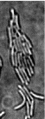
(a)

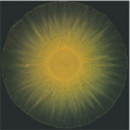
(b)

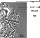
(c)

Figure 1: a) Myxobacteria aligned together into a cluster. Picture obtained in Dr. Shrout’s lab by Cameron Harvey. b) Swarm of M. Xanthus, picture taken by Lotte Jelsbak. The edge of the swarm displays a single layer of cells that are spreading outwards away from the cell center Kaiser07 c) Distribution of cells at the swarm edge Wu09 . The multicellular structures, slime trails, mounds, and rafts are labeled. The swarm is expanding in the radial direction, which is to the right of the image.

Recent two-dimensional (2D) off-lattice microscopic stochastic model (MSM) described in Wu07 , has been able to predict optimal reversal rates for specific choices of bacterial velocities and aspect ratios leading to the maximal swarming rates of the colony, which were confirmed in experiments Wu09 . It has been also shown in Wu09 that such choice of the optimal reversal rate allows cells to align better and resolve traffic jams resulting in the maximal order of alignment. The model takes into account cell shape and direction of motion of each Myxobacteria in the colony determined by the two motility mechanisms: pili VI and slime production. Such detailed cell description is computationally intense and makes any analytical description difficult.

Experimental observations suggest that the capacity to swarm depends less on the motility engine employed by individual cells and instead on the behavioral algorithms that enhance the flow of densely packed cells Kaiser07 ; Wu09 . Because of that we focus in this paper on the study of self-propelled motion of rod shaped bacteria without specifying motility engines. We do not incorporate cell division, the directional effects of slime, or the social motility governed by pili into the model. Instead we use a basic model for studying mechanism of swarming caused by the cell-cell collisions (jams) and regular cell reversals, in a small part of the colony near the edge of the swarm where motion of bacteria is nearly one-dimensional in the radial direction (see Fig. 1). We assume that cells cannot climb onto each other and that no more than one cell could be positioned at any moment in time at specific location in space (by using excluded volume constraint). Cells are modeled as self-propelled bending rods which glide on slime on the substrate with the same constant velocity. They reverse direction of their motion periodically in time which serves as a mechanism for diffusion of spatial positions of cells.

The main result of the paper is an establishment of a connection between one-dimensional (1D) microscopic and macroscopic models and and their parameters, describing swarming of bacteria reversing at different frequencies. Microscopic 1D discrete stochastic model is a 1D simplified version of the full 2D model Wu07 . 1D macroscopic model is a nonlinear diffusion equation for cellular density describing dynamics of self-propelled non-overlapping rods with regular reversals. Combination of a stochastic discrete model and its continuous limit in the form of a nonlinear diffusion equation constitutes a multi-scale modeling environment which allows one to zoom in and study individual bacteria and then zoom out and investigate emerging behavior of a large number of bacteria in a swarming colony.

Although, only few continuous models based on biological cell behavior exist which take volume of cells into account and prevent cells from overlapping, such models are more biologically relevant and can provide novel insights. Recently continuous limit models describing dynamics of cellular density were derived from the microscopic motion of randomly moving cells exhibiting volume exclusion and chemotaxis Alber06 ; Alber07 ; Lushnikov08 . In particular, the Ref. Lushnikov08 introduces a nonlinear diffusion equation model with chemotactic term for describing amoeba aggregation without blow up of solution in finite time Alber09 . This is in contrast with the standard but biologically less realistic Keller-Segel equation (sometimes also called Patlak-Keller-Segel equation) with constant diffusion coefficient Patlak1953 ; KeSe1970 which neglects the size of bacteria resulting in solution (bacterial density) having a blow up (collapse) in finite time BrCoKaScVe1999 ; LushnikovPhysLettA2010 ; DejakLushnikovOvchinnikovSigalPhysDSubmitted2010 .

Another 1D continuous limit equation was recently derived from a model of cells that interact using Hooke’s Law Murray09 . This equation also displays nonlinear fast diffusion, and looks similar to the porous medium equation but with a negative exponent. This model agrees well with the discrete system from which it is derived and it is capable of effectively making biological predictions for cells that can be modeled as stiff springs.

The paper is organized as follows. In Section II a Microscopic Stochastic Model (MSM) of cellular dynamics is introduced which describes 1D motion of sell-propelled rods with periodic in time reversals of the direction of their motion. In Section III general settings for MSM simulations are presented and results of multiple 1D dynamics MSM simulations with initially localized distributions of bacterial colonies are described. In Section IV elementary laws of collisions (jams) between cells are derived and equilibrium motion of cells is determined in the limit of zero noise of the reversal period. Without interactions (in a vanishing cell density limit) each cell experiences almost periodic motion in space and time. Without a noise in the reversal time that motion would be strictly periodic. However, the experimentally observed Welch01 small noise in the reversal time results in the random walk of the average position (averaged over time period $2T$) of the center of mass of each cell at time scales above $2T$. Here $T$ is the average reversal time for each cell. For finite cellular densities we introduce different types of collisions (jams) between cells including pairwise jam and cluster jam. We also find the critical density $p_{0}$ below which cellular diffusion is dominated by the diffusion (random walk) of individual cells while above $p_{0}$ the diffusion is dominated by the collisions between cells. In Section VI multiple collisions and cell clustering for large cellular densities are studied. In Section VII a nonlinear diffusion equation of the general form

$$\partial_{t}p=\partial_{x}\Big{[}D(p)\partial_{x}p\Big{]},$$ (1)

is introduced, where $p(x)$ is a local cell density (measured in units of volume fraction, i.e. the ratio of volume occupied by cells to the total volume of space), $x$ is the spatial coordinate and $D(p)$ is the nonlinear diffusion coefficient determined by using Boltzmann-Matano (BM) analysis BoltzMat of ensemble averaged MSM simulations of cells moving with different reversal frequencies. The equation (1) gives microscopically averaged dynamics of cellular density vs. microscopic description of MSM model. We compare the dynamics of cellular density from MSM simulations with the numerical solutions of the equation (1) for different reversal frequencies and find very good agreement between these two types of simulations for $p>p_{0}$. This confirms that the dynamics of cellular density is indeed of a nonlinear diffusion type (1). In Section VIII an analytical approximation for pairwise collision time and semi-analytical fit for the total jam time per reversal period are described. In Section IX main results of the paper and future directions are discussed. In Appendix A Boltzmann-Matano analysis is reviewed. Appendix B provides additional testing of the accuracy of Boltzmann-Matano approach for the cellular distributions of finite size.

II Microscopic Stochastic Model of Bacterial Motion

In this section we introduce a computational discrete microscopic stochastic model (MSM) of cellular dynamics describing motion of self-propelled rods on a 1D lattice with periodic in time reversals of the direction of their motion.

We simulate constant number of cells of length $L$ that move back (left) and forth (right) in a spatial domain along the coordinate $x$ with periodic boundary conditions and velocity $v$. We assume that each cell reverses the direction of its motion in average time $T$ after previous reversal. The reversal period experiences fluctuations with the variance $\Delta T_{0}^{2}$ which are sharply peaked near $T$, i.e. $\Delta T_{0}/T\ll 1$ in accordance with the observed in experiments Welch01 . Assume that the positive integer $n$ corresponds to the $n$th reversal of the given cell. We chose the probability distribution for the stochastic realizations of the reversal time $T_{n}$ for $n$th reversal to be defined through the Poisson distribution

$$f(k)=\frac{\lambda^{k}e^{-\lambda}}{k!},\quad k=0,1,2,\ldots$$ (2)

as follows

$$T_{n}=k\Delta T_{1},$$ (3)

where $\lambda=T^{2}/\Delta T_{0}^{2}$ and $\Delta T_{1}=\Delta T_{0}^{2}/T$. Because the statistical averages for (2) are $\langle f(k)\rangle=\lambda$ and $\langle(f(k)-\langle f(k)\rangle)^{2}\rangle=\lambda$ we obtain that $\langle T_{n}\rangle=T$ and $\langle(T_{n}-\langle T_{n}\rangle)^{2}\rangle=\Delta T_{0}^{2}$. With that definition the stochastic realizations of $T_{n}$ can take only discrete values $0,\Delta T_{1},2\Delta T_{1},\ldots$. But because we assume $\Delta T_{0}/T\ll 1$ we conclude that this is a good approximation of the Myxobacteria reversals with continues set of values of the reversal time.

To quantify the difference between reversal times of neighboring bacteria we introduce the reversal phase for each bacteria defined as follows. We define time periods $(0,2T)$, $(2T,4T)$, $(4T,6T)$ etc. Inside each of these intervals each cell (bacteria) has an assigned reversal phase, $\phi$, between $0$ and $2T$ corresponding to the time when cell reverses from moving to the right to the motion to the left (i.e. cell reverses from right-directed motion to the left-directed at times $t=\phi,\,2T+\phi,\,4T+\phi,\ldots$). Reversal in opposite direction occurs at at times $t=\phi,\,T+\phi,\,3T+\phi,\ldots$. The initial phase of each cell is chosen at random. Here the phase $\phi$ is not constant but changes after each reversal because of fluctuations of $T_{n}$. The condition $\Delta T_{0}/T\ll 1$ ensure that the change of $\phi$ at the time scale $T$ is small. Respectively, at much larger time scale $t\gg T$ the phase $\phi$ experiences the random walk. These random walks are independent for for each of $N$ cells in the system.

In dimensionless units we assume that $L=1$ and $v=1$. Unless otherwise specified we choose $T=8$. Each cell is represented by a finite number of lattice sites on a 1D grid. In a typical simulation, each cell includes 10 lattice sites, i.e. distance between neighboring lattice sites is $\triangle x=0.1$ (see Figure 2 a). Time step in dimensionless units is $1/\triangle x$ to keep the velocity $v=1$. However, we also ran multiple simulations with smaller values of $\triangle x$ to make sure that increasing number of lattice sites per cell (but keeping $L=1$ and decreasing time step to keep $v=1$) does not significantly change our results . In other words, we look at the continuous limit as $\triangle x\to 0.$

The following three dimensionless parameters completely determine the dynamics of cells in continuous limit $\triangle x\to 0.$ The first parameter is $vT/L,$ which is the ratio of the average distance traveled by cells between reversals and the cell length. That parameter is $vT/L=8$ for the typical value $T=8$. The second dimensionless parameter is the local cellular density $p(x)$ measured in units of volume fraction $p$, i.e. the ratio of volume occupied by cells to the total volume of space (in 1D, volume is simply the length). The third parameter is $\Delta T_{0}/T$, i.e. relative size of the reversal time fluctuations.

For example, we can choose the velocity, the reversal period, the fluctuation of the reversal period and the cellular length as $v_{dim}=10\mu m/min$, $T_{dim}=8$min, $\Delta T_{0,dim}=0.9$min and $L_{dim}=10\mu m$, respectively, in dimensional units. This yields $v_{dim}T_{dim}/L_{dim}=8$ similar to the typical dimensionless values chosen above. This choice is consistent with cell lengths and reversal period used in previous computational models Wu07 ; Wu09 and observed in experiments Myxobacteria . Below unless otherwise specified we choose $\Delta T_{1}=0.1$. For $T=8$ it corresponds to $\Delta T_{0}\simeq 0.9$. Experiments with Myxobacteria typically show only small fluctuations of the reversal period $T$ so that probability distribution function is sharply peaked near average reversal period $T$ Welch01 . Our typical choice $\Delta T_{0}\simeq 0.9$ reflects that smallness of fluctuations. We also checked that if there is no noise added to the reversal period, the simulations fails to match the nonlinear diffusion equation (1). This suggests that noise (although small) in the reversal period of bacteria contributes to their macroscopic behavior by allowing them to behave diffusively.

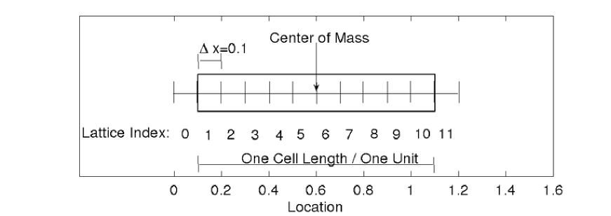
(a)

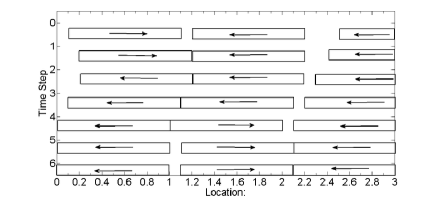
(b)

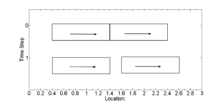
(c)

Figure 2: a) Diagram of a single cell with marks designating absolute location versus lattice index. b) Sample movement in a single time step where one cell is chosen twice and the other is not chosen at all. c) Sample movement of three cells where each cell is chosen exactly once.

At each time step, the model determines cell movement based on the occupancy of the next lattice site in the direction the cell is moving (direction is determined by $\phi$ at the given time $t$). If this location is free, the cell is moved 1 lattice site in that direction (keeping constant length $L=1$). If the location is not free, the cell does not move.

The model itself is stochastic. During each time step, a sequence of $N$ randomly chosen cells attempt to move one at a time, where $N$ is the total number of cells. It is possible that the same cell may move more than once during a time step, and as a result some other cells may not move at all. Also, note that random selection of cells may create gaps between cells that are following each other (see Figures 2b and 2c for examples of possible cellular movement). Creation of such gaps is equivalent to the extra diffusion each cell experiences in addition to the directed motion with the speed $v$. That diffusion is a pure artefact of the finite width $\triangle x$ of each lattice site which vanishes as $\triangle x\to 0.$ We checked in simulations that reduction of $\triangle x$ from 0.1 to 0.001 gives only small changes in the cellular density dynamics (see Section VII.2 for more discussion on that). However, the collision time between cells is more sensitive to the value of $\triangle x$ so for these type of simulations in Section VIII we also used grid spacing down to $\triangle x=0.001$. Generally, in all quantities plotted in all Figures of the paper we choose $\triangle x=0.1$ unless we explicitly specify a different value of $\triangle x$.

Unless otherwise specified, the simulations are run on a one-dimensional lattice domain of length $4,000$ centered at $x=0$ starting with an initial top-hat distribution of cells of width $1,000$ also centered at $x=0$ (i.e. density of cells is approximately constant $p\equiv p_{max}$ for $-500<x<500$ and zero everywhere else). See curve for $t=0$ in Figure 3a as example of a top-hat boundary condition. Because the domain is symmetric between $x$ and $-x$ it replicates a no-flux boundary condition at $x=0$ after averaging over the statistical ensemble of simulations. Generally, we choose lattice domain of length large enough to have no influence of the periodic boundaries (i.e. to have zero cellular density at both right and left boundaries).

III MSM Simulations

Swarming of bacterial colony similar to the one shown in Figure 1a can be analyzed by averaging over angles, i.e. as an average over dynamics of many nearly 1D (in the radial direction) distributions of Myxobacteria. In what follows we assume that motion along radius is a dominant one while rotation is only a correction which we neglect here.

We performed multiple MSM simulations of 1D dynamics of initially localized distributions of bacterial density and performed ensemble averaging over these simulations. The ensemble serves to approximate averaging over angles or the full 2D problem. We choose the ”top-hat” initial distribution (constant density around the center of the domain and zero density to the left and to the right of the center). Initial top-hat density profile was typically obtained by a dense initial packing of bacteria in the domain of width 1000 around $x=0$. The typical size of a statistical ensemble was $20,000$. We determined the cellular density (volume fraction) by calculating the average number of times the given location was occupied (see Figure 3a). Qualitatively, the cell densities spread out symmetrically away from the center of the top hat. For later times a steep slope develops around density $p_{0}=0.2$, which implies that the rate at which the density spreads out depends on the local cell density.

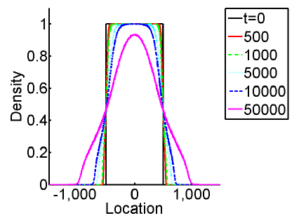
(a)

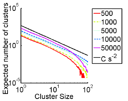
(b)

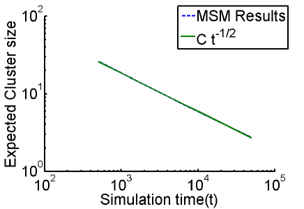
(c)

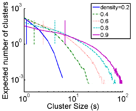
(d)

Figure 3: Results of MSM simulations of rods reversing every T=8 performed $20,000$ times. (a)-(c) to correspond to simulations with top-hat initial conditions and (d) corresponds to simulations with initial constant average density. (a) Average cell density at different times. (b) Expected cluster frequencies for different times, i.e. the average number of clusters of a given size obtained in the simulations. (c) Average cluster size over time on a log-log scale. (d) Expected cluster frequencies at end time $50,000$, after cooking initial conditions, for constant density simulations of ensemble size $2,000$, where the vertical bars signify the average cluster size.

The cells’ movement frequently causes them to collide with each other. When two cells are trying to move into each other’s space, they stall (jam) until at least one reverses. This stalling, on average, shifts the mean location of their oscillatory movement away from the location at which they stall. If no other cells are nearby, the cells may collide again or separate further away due to fluctuations in the mean location of their oscillatory movement. If other cells are nearby, these outer cells have their mean location shifted outwards while the original cells’ mean locations are shifted closer together. Through these shifts, the cells steadily spread away from each other.

In highly packed situations, the cells cluster together. Two cells can jam together forming two-cell cluster, and if another cell is moving in a direction of a that two-cell cluster then it may join the cluster forming three-cell cluster etc. To measure the amount of clustering, we calculated the frequencies of cluster sizes at different moments of time which is shown in log-log plots in Figure (3b) for MSM simulations with top-hat initial conditions. It is seen that the frequency of cluster sizes follows $-2$ power law. It is seen that the average cluster size decreases over time as initially densely packed cells expand. Figure (3c) shows that this decrease follows a power law decay over time with calculated exponent $-0.4965$ which is close to $-1/2$ power laws expected from diffusion.

This suggests that during early times, many of the cells are found in large clusters where they cannot move. At later times, the large clusters rapidly break up into smaller clusters allowing cells to move. Also, the individual cells near the boundaries spend a significantly greater percentage of their time moving.

Figure 3a shows that the dynamics of the cellular density is smooth and slow compare with the velocity $v=1$ of individual cell motion. It suggests the ensemble averaged distribution of cells at each moment of time and at each point in space is in statistical quasi-equilibrium. Below we study dependence of quasi-equilibrium on local cellular density, cellular collision times and cluster sizes. We also performed a second type of MSM simulations with periodic boundary conditions and uniform average densities to study statistical equilibrium of cellular motion.

IV Elementary laws of collisions (jams) between cells and equilibrium motion of cells in the limit of zero noise of the reversal period

If the noise in the reversal time $T$ is absent then in a vanishing cell density limit each cell experiences periodic motion in space and time with its center of mass not moving on average (after averaging over time period $2T$). However, the experimentally observed Welch01 small noise in the reversal time results in the random walk of the average position (averaged over time period $2T$) of the center of mass of each cell at time scales above $2T$. That random walk results in collisions of cells for any finite density. As density goes to zero these collisions become more and more rear because it takes more time for cells to span the average distance between them through random walk. Below in this Section we consider the limit when we completely neglect that random walk, i.e. we neglect the noise in $T$.

For nonzero density of cells, there is a finite probability for two neighboring cells to collide (jam). By jam, we mean that one cell tries to move where another cell is located, but the excluded volume principle prevents them from moving. The term ”jam” in this paper is similar to the term ”collision”. The subtle difference is that by collision we mean that a cell jams with another cell with subsequent unjamming, i.e. the cell is free to move after a jam.

We distinguish two types of jams. First type is a “pairwise jam”. It occurs when two neighboring cells are jammed directly because they try to move in opposite directions towards each other but that motion is prevented by the excluded volume principle. Second type of jam occurs when a cell 1 tries to move in the same direction as a neighboring cell 2 but that cell 2 is jammed by another cell(s) (e.g. by cell 3). We refer to such type of a jam of cell 1 as “indirect jam”. Such jam is an indirect one because there is no direct (pairwise) jam between cells 1 and 2. A typical example is when cell 1 moves towards neighboring cell 2 while cells 2 and 3 have a pairwise jam. After cell 1 touches cell 2 they together (cells 1,2 and 3) form three-cell cluster with pairwise jam between cells 2 and 3 and indirect jam with cell 1. We also say that a given cell is in a “cluster jam” if it is either pairwise or indirect jam. The pairwise collision time $\tau_{pair}$ is always smaller or equal to $T$ because of reversal of the direction of cellular motion. In contrast, the cluster jam time $\tau_{cluster}$ can be arbitrary large if cells stay inside of a large cluster. Also in Section VIII we use total jam time $\tau$ per period $T$, i.e. the time during which a given cell remains jammed (either directly or indirectly) per period $T$. With such definition $\tau$ never exceeds $T$.

Assume that density is small so that mostly pairwise jams occur. In such a case jamming of two cells lasts until one of the cells reverses. After that they move together in the same direction until the second cell reverses. After the second cell reversal, cells move in opposite directions away from each other. Assume that all other cells are still far away. Then after the first cell reverses for a second time both cells will move in the same direction, and after the second reversal of the second cell they will move towards each other. Exact calculation shows that these two cells will never jam again in the absence of other cells. Instead, exactly at the moment when these two cells touch each other, the first cell will reverse for a third time and they will move in the same direction again. This pattern of periodic motion without jamming of these two cells will continue for arbitrary long time (or until another, third cell, would approach them close enough to jam with one of these two cells). It means that any two isolated cells jam only once and after that both cells will experience periodic motion without disturbing one another.

A similar interaction pattern occurs if we consider a system of three or more cells moving in an infinite spatial domain. After several collisions (jams) between these three or more cells, they will also end up in the state where they will not jam any more and all cells will experience periodic motion without touching each other. A center of mass of each cell participating in a jam shifts relative to its average position at a distance $v\tau_{pair}$ to the left or to the right (depending on which side it has a jam), where $\tau_{pair}$ is the collision time. However, after all collisions are over, center of mass of each cell experiences periodic motion and no average motion (averaged over the period $2T$) is observed. We refer to such state as an equilibrium motion of Myxobacteria. Note that equilibrium motion is quite different from the equilibrium distribution (Gibbs distribution) in statistical mechanics LandauLifshitzStatisticalPhysics1980 because Myxobacteria are always self-propelled and are not subject to any type of thermal equilibrium. Starting with a finite number of initially densely packed Myxobacteria, after finite number of collisions and provided Myxobacteria divisions are neglected, the bacterial colony expands to such size that there will be no more collisions between cells. After that the average size of the colony remains the same with bacteria moving periodically at equilibrium.

We now calculate the density of Myxobacteria $p_{0}$ at which a transition occurs from motion with collisions to equilibrium motion. First, consider two neighboring cells and assume that they have phases $\phi_{1}$ and $\phi_{2}$, respectively. Generally $-2T\leq\phi_{1}-\phi_{2}\leq 2T$ but assuming periodicity over time $2T$ we can always add a multiple of $2T$ to each of the phases, $\tilde{\phi}_{j}\equiv\phi_{j}+n_{j}2T$, $j=1,2$ ($n_{j}$ are integers), to keep the difference of modified phases inside a twice smaller interval: $-T\leq\tilde{\phi}_{1}-\tilde{\phi}_{2}\leq T$. For $p=p_{0}$ cells do not jam but during a part of the time interval $2T$ they move together (attaching to each other) in the same direction until one of them reverses. After that, they move in opposite directions from each other for the time interval $|\tilde{\phi}_{1}-\tilde{\phi}_{2}|$. After that second cell reverses and both cells move in the same direction etc. Minimum separation between centers of mass of these two cells is $L$ and maximum separation is $L+2v|\tilde{\phi}_{1}-\tilde{\phi}_{2}|$. So the distance $L_{dist}$ between the average positions of centers of mass is $L_{dist}=L+v|\tilde{\phi}_{1}-\tilde{\phi}_{2}|$. Now, to calculate the average density $p_{0}$ of many cells we average $L_{dist}$ over phase differences $0\leq|\tilde{\phi}_{1}-\tilde{\phi}_{2}|\leq T$ resulting in the critical density

$$p_{0}\equiv\frac{L}{\langle L_{dist}\rangle}=\left[T^{-1}\int^{T}_{0}(L+v\phi)d\phi\right]^{-1}=\frac{L}{L+vT/2}.$$ (4)

For the standard values $v=L=1,\ T=8$ it yields that $p_{0}=0.2.$

If initially there is a localized distribution of cells with the average density $p>p_{0}$, then these cells will spread out with collisions until their density reaches $p=p_{0}.$ If initially $p<p_{0}$, then some redistribution of cellular density may occur when the average distance between centers of mass of two neighboring cell is $L_{dist}<L+v|\tilde{\phi}_{1}-\tilde{\phi}_{2}|$. Because average density is low, this would result only in a local redistribution of the positions of cells without much change in the macroscopic cellular density. After initial spreading out no collisions or cellular density transport will be observed.

We conclude that in order to observe transport of a system of self-propelled rods without noise in the reversal period $T$ at long times one needs to incorporate in the model a source of the density gradient. In Myxobacteria swarms, such a source is present because of division of cells in the center of the bacterial colony. Thus any transport of self-propelled rods without noise in $T$ is a collective phenomena with the threshold density $p_{0}$ required for transport.

V Re-introduction of the noise of the reversal period in the small density limit

We now take into account the noise of the reversal period $T$ in the analysis of the previous Section. In that case collisions between cells occurs even for $p<p_{0}$ because random walk of the average position of cells causes them to move at arbitrary large distance until finally colliding with other cells. When density approaches to zero the frequency of collisions also goes to zero. But if $p\to p_{0}$ from below then cells collide typically at each period $2T$ with the collision time $\sim\Delta T_{0}$ (so that for $\Delta T_{0}\to 0$ that collision time would vanish). Thus $p_{0}$ separates two regime of collisions: for $p<p_{0}$ rare collisions primary occur because of the noise of $T$ while for $p>p_{0}$ collisions are dominated by frequent collisions. At the transition densities $p\sim p_{0}$ the contributions of both of these effects are comparable.

Thus a transport of Myxobacteria is a mixture of two effects. First effect is the diffusion of individual cells due to the noise in the reversal period $T$ which dominates for small densities $p<p_{0}$. Second effect is due to the frequent collision of cells during each period $2T$ making that effect essentially collective one. These two regimes make Myxobacteria quite distinct from bacteria like E. Coli or amoeba Dictyostelium discoideum which experience diffusion as random walk of Brownian-like particles Alber06 ; Alber07 ; Lushnikov08 without any periodic motion.

VI Multiple collisions and cell clustering for large cellular densities

If the cellular density $p$ is not small ($p>p_{0}$) so that cells typically experience collisions during each period $2T$, then cell motion is more complicated than described in Section IV which is based on rare pairwise collisions. In addition we assume here and below that there is nonzero noise in $T$ as in Section V. Figures 4(a-d) show pairwise jam time (jam duration) versus collision number that occur between three adjacent cells for the average cellular density $p=0.95$. In that case cells occupy 95% of total volume and between two reversals each cell can cover up to $vT/L=8$ cell volumes meaning that it could collide with multiple cells if allowed to. It is shown in Figure 4 that distribution of pairwise jam time $\tau_{pair}$ is random. Such regime typically occurs closer to the bacterial colony center where cell flux caused by cell divisions is large and it keeps the system far from equilibrium motion state as described in Section IV.

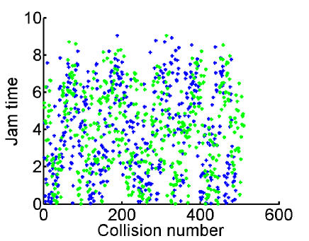
(a)

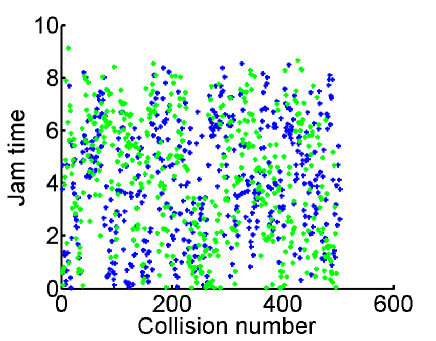
(b)

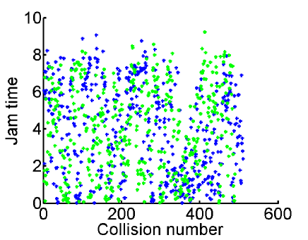
(c)

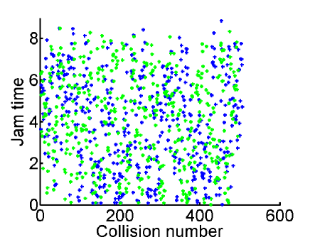
(d)

Figure 4: (a-d) Four stochastic realizations of the pairwise jam time that a single cell experiences with its two adjacent neighbors. Collisions with the left and right neighbors are colored blue and green respectively for a total of 1,000 different collisions at average cellular density 0.95 and $\triangle x=0.001$.

There are at least two situations where such a far from equilibrium state is possible. First is the high density gradient case caused by bacterial division (as mentioned above). The second case occurs if no-flux boundary conditions maintain a large density of Myxobacteria in a domain with fixed volume. In both cases the rate of bacterial jamming is high and the collision times are randomly distributed.

Another effect which occurs in case of large densities is the high probability of formation of clusters consisting of more than two bacteria. As density of bacteria approaches one, all bacteria jam in large clusters. Unjamming bacteria from large cluster might take a lot of time because leftmost or rightmost bacteria in the cluster need to move away providing space for the bacteria in the center of the cluster to move in. As a result, many cells stay jammed in a cluster for a long time for large densities. Figure 5 shows that the average cluster collision time $\tau_{cluster}$ (averaged over ensemble of MSM simulations) diverges for $p\to 1.$ Values of $\tau_{cluster}$ for different $\Delta x$ show good convergence to the continuous limit $\Delta x\to 0$. E.g., curves for $\Delta x=0.01$ and $\Delta x=0.001$ are almost indistinguishable.

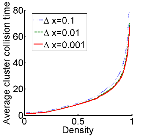
Figure 5: Average cluster collision time $\tau_{cluster}$ as a function of density $p$ for different values of $\Delta x$. It is seen that $\tau_{cluster}\to\infty$ for $p\to 1.$

Figure 3b shows the distribution of cluster sizes for MSM simulations starting from a top-hat initial condition. Figure 3d shows the cluster size distribution for different densities $p$ for MSM simulations with uniform average density and periodic boundary conditions (second type of MSM simulations is described in Section III.

VII Macroscopic Nonlinear Diffusion Model and MSM simulations

VII.1 Nonlinear Diffusion Model and Its Limitations

If collisions are frequent and, additionally, the distribution of the reversal phases and initial position of cells are random, then we assume that collective dynamics of cells is diffusion-like and it is described by the equation of the general type (1). In this section, we obtain a numerical approximation of the diffusion coefficient $D(p)$ in (1) to match the results of MSM simulations. This is achieved by running MSM simulations with a top-hat initial distribution and using Boltzmann-Matano (BM) analysis BoltzMat applied to the ensemble-averaged MSM density profile on the right half of the spatial domain at time $t=t_{D}$. Here and below $t_{D}$ describes the time at which we apply BM analysis. (Description of the BM analysis is given in Appendix A). Then we demonstrate that numerical solutions of (1) with $D(p)$ obtained using BM analysis, yield density dependence on space and time which are in a very good agreement with the one obtained using MSM simulations, justifying initial assumption of collective dynamics of cells being diffusion-like.

Results of MSM simulations unavoidably have noise due to the finite size of stochastic ensemble used to determine cellular densities. BM analysis relies on calculating derivatives of density and we apply Gaussian filter to the MSM density data to smooth out both $p$ and all its derivatives nixon2008feature . We checked that the change of parameters of the Gaussian filter resulted in only small corrections without any systematic error.

Typically, to perform BM analysis we run MSM using an initial top-hat distribution of length $1,000$ in a domain of size $4,000$ (see the end of Section II for more details). For most of our simulations, the top-hat is wide enough so that during simulation time the density at the middle of the domain remains close to the initial density $p_{max}$ (in most simulations $p_{max}=1$). It means that cells mostly move near the boundary of initial top-hat distribution while at the middle of the domain the cellular density is almost constant. This allows us to ignore the left half of the domain and treat the cell distribution as if it were step-wise shaped in an infinite domain. This is necessary in order to perform BM analysis which is exact for infinite spatial interval with step-wise initial conditions only. In Appendix B we study the accuracy of BM analysis for a finite width of top-hat initial conditions.

Another limitation of the BM analysis is that it requires calculating $(dp(x)/dx)^{-1}$. Due to the presence of the regions where the density is constant, singularities of $(dp(x)/dx)^{-1}$ may be generated in the calculation of the non-linear diffusion coefficient near the end of the diffusion curves where $p$ is close to 0 or $p_{max}$. These artificial singularities result from a loss of numerical precision near singularity of $(dp(x)/dx)^{-1}$ which is clearly seen near $p=0$ and $p=1$ in all Figures below that include $D(p)$. To reduce such loss of numerical precision we only perform BM analysis in the neighborhood of the interface that encompasses the initial step of a top-hat instead of the entire right half of the domain. It can be also mitigated by performing a cubic spline interpolation of $D(p)$ from the domain $0<p<1$ to values around $p=0$ and $p=1$. This, however, appears to be not necessary because the loss of precision does not affect prediction of the density dynamics in (1) in any significant way.

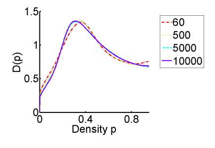
(a)

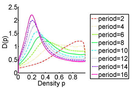
(b)

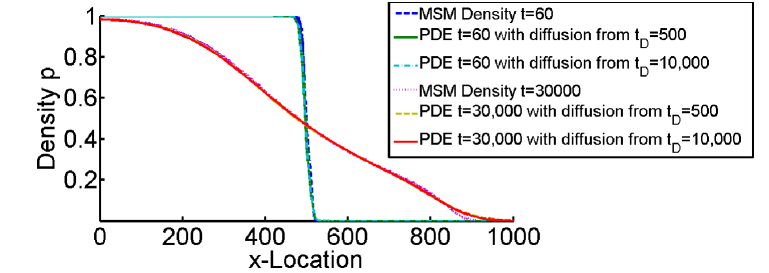
(c)

Figure 6: (a) Diffusion coefficient $D(p)$ generated by BM analysis at different times $t_{D}$ for $T=8$. (b) $D(p)$ generated by BM analysis for varying reversal periods $T$ for diffusion curves calculated from BM analysis at $t_{D}=500$. (c) Density profiles from MSM simulations vs. PDE density profiles (solutions of (1)) at $t=60$ and $t=30,000$ obtained using diffusion coefficients from (a) with $t_{D}=500$ and $t_{D}=10,000$. It is seen that the fit between two types of density profiles is very good except the region of small density $p<p_{0}=0.2$.

Since the BM analysis approach for calculating the diffusion coefficient assumes that the nonlinear diffusion equation (1) is solved on an infinite domain, there will be errors in calculating the diffusion coefficient if there is significant density near the boundaries of our finite computations domain. So if were to choose $t_{D}$ that is too large, the analysis would fail. Also, if were to choose $t_{D}$ that is too small, then not enough cells would reverse to generate diffusion. We found that any time between $t_{D}=125$ and $t_{D}=10,000$ appears to be sufficient for generating reasonably universal diffusion curves for $T=8$ as shown in Figure 6a. In other words, diffusion coefficient curves $D(p)$ generated at different times $t_{D}$, are close to each other. This near-independence of $D(p)$ from $t_{D}$ justifies our assumption of the collective dynamics of cells being diffusion-like and described by (1).

Small difference between different diffusion curves $D(p)$ generated at different times $t_{D}$, is due to the absence of diffusion for $p<p_{0}$, where the critical density $p_{0}$ is defined in (4). For $p<p_{0}$ there are practically no jams between cells (see Section IV) and, subsequently, there is no diffusion. (Some occasional jams are still possible only because cells are not in fully quasi-equilibrium and because of finite value of $\triangle x$.) BM analysis assumes that $D(p)$ is an analytical function. But a sharp drop of diffusion to zero for $p<p_{0}$ breaks that analyticity. Therefore, in BM analysis approach a drop of $D(p)$ from finite value at $p\to p_{0}+0$ to the zero value at $p\to p_{0}-0$ is replaced by a smooth function shown in Figures 6a and b (see also Section VIII for more relevant discussion on this subject). Thus, nonzero values of $D(p)$ for $p<p_{0}$ in Figures 6a and b are artifacts of the BM method. Also, finite values of $\triangle x$ contribute to nonzero value of $D(p)$ for $p<p_{0}$ but that contribution is small for $\triangle x\leq 0.1$ in comparison with contribution of BM analysis. In the limit $\triangle x\to 0$ there is no average macroscopic motion of cells for $p<p_{0}$. MSM simulations indicate this by the sharp drop of density for $p<p_{0}$. (Such drop is not completely vertical because of finite sizes of cells in the MSM.) In addition, macroscopic averaging requires taking into account a finite spatial width of that sharp drop of density. We conclude that the difference between MSM and PDE curves in Figure 6c for $p<p_{0}$ is due to the limitation of applicability of BM analysis for $p<p_{0}.$

Unless otherwise specified below we use $t_{D}=500$ to generate the diffusion curves.

To demonstrate that there is little difference in the solutions of (1) with diffusion coefficients $D(p)$ chosen based on BM analysis with $t_{D}=500$ versus $t_{D}=10,000$, we compare the resulting numerical solutions with the densities obtained using microscopic stochastic model simulations (see Figure 6c). Figure 6c shows that PDE density profiles $p(x)$ are almost indistinguishable for both values of $t_{D}$. Furthermore, the difference between the numerical solutions of the nonlinear diffusion equation and stochastic simulation results are negligible except for the region $p<p_{0}$.

Diffusion curves for different reversal periods $T$ were also calculated (see Figure 6b). Large reversal periods $T$ produce high diffusion at low densities, and low diffusion at high densities. Small reversal periods produce low diffusion at low densities and high diffusion at high densities. In the former case the cells move left or right until they collide and they stay jammed for a long time. In the later case, the cells rapidly oscillate left and right. Once the cells spread out, collisions become infrequent.

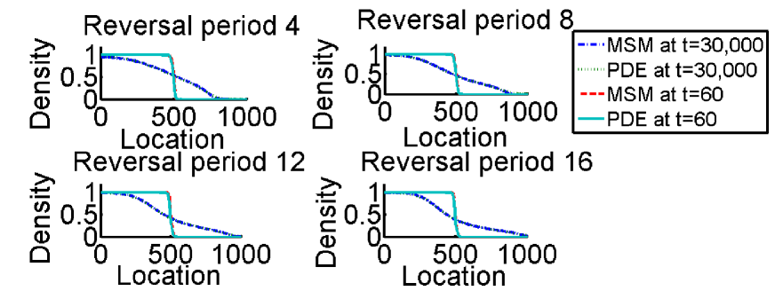
Figure 7: Numerical solution of the diffusion equation (1) (with $D(p)$ from BM analysis) plotted against the ensemble-averaged MSM results at $t=60$ and $t=5,000$ for different reversal periods $T$. PDE and MSM results are almost indistinguishable.

VII.2 Testing accuracy of the nonlinear diffusion model and macroscopic limit of MSM

To test that the diffusion curves in Figure 6b actually predict the diffusion in the stochastic model, we compared numerical solutions of the diffusion equation (1) with $D(p)$ derived using BM analysis of MSM simulations with different reversal periods at an early and a later times (see Figure 7). Very good match is demonstrated for $p>p_{0}$, where the critical density $p_{0}$ is defined in (4).

To test whether the dynamics of the discrete stochastic system is consistently well approximated by the diffusion equation, independently of initial density, we compared the numerical solutions of the diffusion equation with the MSM simulations for $T=8$ reversal period and different initial conditions (different amplitudes of densities in the initial top-hat profile).

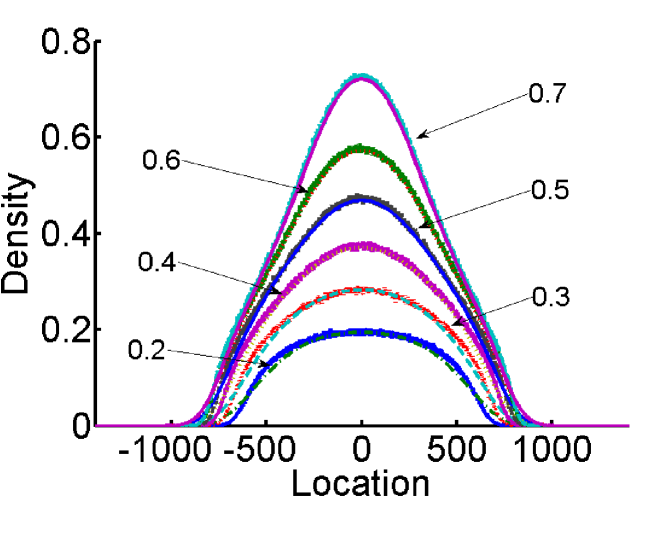
Figure 8: Comparison of ensemble-averaged MSM simulations with numerical solution of (1) (with $D(p)$ from BM analysis) using different initial densities. MSM densities are not smooth because of finite size of statistical ensemble. It is seen that PDE results are well approximations for MSM for $p>p_{0}$ if we average over fast fluctuations of MSM densities. Simulations results were taken at $t=50,000$

We first generated random initial conditions with constant average density and periodic boundary conditions and allowed cells to move in the MSM simulations for $t=50,000$ to reach statistical equilibrium. After that we inserted the obtained equilibrium distribution as a top part of top-hat initial condition and run MSM simulations starting with these spatially nonuniform initial conditions. Figure 8 shows a very good match between these simulations and numerical solutions of the nonlinear diffusion equation. Matching is not as good for smaller densities due to the qualitative change of diffusion and lack of collisions for $p<p_{0}$ as was explained above.

Since cells move on a discrete grid at discrete time steps, we test convergence of the system to a continuous description of cell movement by decreasing the grid spacing $\triangle x$, and by scaling the lengths and time steps appropriately. The results of the ensemble-averaged MSM simulations for the spatial profile of density are shown in Figure 9. It is seen that the reduction of $\triangle x$ from 0.1 to 0.001 results only in small changes in the cellular density dynamics with density curves for different $\triangle x$ practically indistinguishable in Figure 9. It suggests $\Delta x=0.1$ is already a quite good approximation for the cellular dynamics in continuous limit.

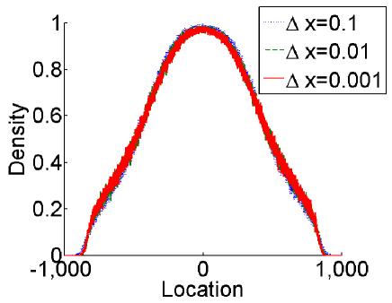
Figure 9: Spatial distribution of density at $t=30,000$ from the ensemble-averaged MSM simulations with different $\Delta x.$ Initial condition had a form of top-hat distribution of width 1000.

The diffusion curves obtained from BM analysis are more sensitive to the change of $\Delta x$ compare with the sensitivity of $p(x)$ at Figure 9. Figure 10 shows the diffusion curves from BM analysis obtained at $t_{D}=500$ from the same MSM simulations as in Figure 9. It is seen that $D(p)$ is relatively well converges for $\Delta x\lesssim 0.01$. These changes in $D(p)$ do not change the efficiency of BM analysis for the prediction of density dynamics as in Figure 6. For all values of $\Delta x=0.1$ the corresponding diffusion curves from BM analysis work well for the density dynamics. The effect of finite $\Delta x$ is only to modify the diffusion through additional $\Delta x$-dependent fluctuations of the reversal time $T$. The cause of such modification is discussed in Section II.

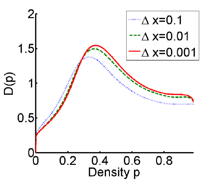
Figure 10: Diffusion coefficient $D(p)$ generated by BM analysis at $t_{D}=500$ for the same simulation as in Figure 9.

We now address the effect of different values of $\Delta T_{0}$. In Myxobactera colony, the fluctuations of $T$ are possible with probability density function for $T$ sharply peaked near average reversal period $T$ Welch01 . We study the role of noise in the reversal period by changing the value of $\Delta T_{0}$. For each $\Delta T_{0}$ we determine the nonlinear diffusion coefficient $D(p)$ using BM analysis BoltzMat of ensemble averaged MSM simulations. We found that $D(p)$ changes with $\Delta T_{0}$ as shown in Figure 11.

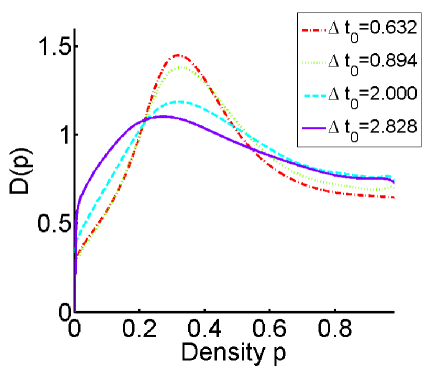
Figure 11: Diffusion curves $D(p)$ for different values of variance $\Delta T_{0}$ of the reversal time $T$ fluctuations (see the equation (3) and after it for definitions) obtained from BM analysis of ensemble-averaged MSM simulations.

Then we compared the density dynamics from MSM simulations and the nonlinear diffusion equation (1). For finite values of noise (typically for $\Delta T_{0}/T_{0}\gtrsim 0.1$) the agreement between (1) and MSM simulations is very good, similar to shown in Figure 6c. When no noise is added ($\Delta T_{0}=0$), we found that (1) is not a good approximation of the density dynamics, i.e. MSM density no longer follows (1) with $D(p)$ from BM analysis as shown in Figure 12.

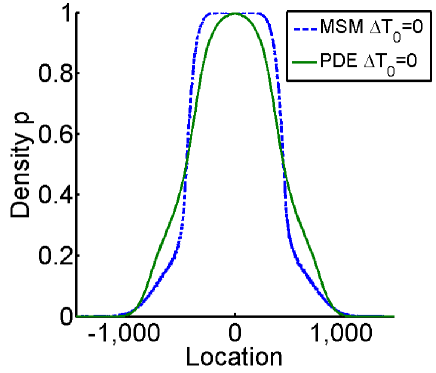
Figure 12: Density curves for MSM simulations with $\Delta T_{0}=0$ and attempted PDE fit using BM analysis at $T=30,000$ and $T_{D}=500$. Initial condition had a form of top-hat distribution of width 1000.

We conclude that the finite noise appears necessary for the nonlinear diffusion approximation to work. Also note that that finite value of $\Delta x$ creates the effective noise in $T$ as discussed above. It means that generally effects of finite $\Delta T_{0}$ and finite $\Delta x$ add up. To distinguish these effects one can reduce $\Delta x.$

VIII Analytical approximations of the pairwise and total collision times

In this section an analytical approximation of the pairwise collision time and semi-analytical fit to the total collision times are derived. We mostly focus on a limit of intermediate cellular density when $p>p_{0}$ but $p$ is not very close to one so that many collisions between cells are still pairwise and they do not result in larger clusters. Assume that a cell experiences on average jam(s) of total duration $\tau_{1}$ from the left and $\tau_{2}$ from the right during each reversal period $2T$. We include both pairwise jams and indirect jams into definition of $\tau$ (see Section IV for detailed definitions of jams). In such a case a shift of the center of mass of a given cell per period $2T$ is $(\tau_{1}-\tau_{2})v$. The average collision time $\tau$ in a given direction (left or right) must be a slow function of $x$ (i.e. $\tau_{1}\simeq\tau_{2}\equiv\tau$) to avoid large microscopic gradients. Typically $\tau$ can be viewed as the average (ensemble or time average) over many collisions (jamming events) for each given cell. It is necessary to stress that $\tau$ in this section is the (total) jam time (from both direct and indirect jams) per period $T.$ This quantity is different from $\tau_{cluster}$ from Section IV because $\tau$ never exceeds $T$ by its definition.

Although jam times can fluctuate strongly from collision to collision (as seen in Figure 4), after averaging over several collisions $\tau$ becomes slow function of $x$ and $t$. We also neglect for now the influence of the fluctuations of the reversal time, i.e. we assume that all reversal phases are constant. Below in this Section we also separately discuss the effect of these fluctuations. Taking into account finite value of $\tau$ we estimate the local cellular density as $p=L/\langle L_{dist}\rangle$, where the average distance between neighboring cells is $L_{dist}=L+v|\tilde{\phi}_{1}-\tilde{\phi}_{2}|-v\tau$ and $\langle\ldots\rangle$ means statistical averaging over the uniformly distributed phases $\tilde{\phi}_{1}$ and $\tilde{\phi}_{2}$. This expression is, however, only true for $|\tilde{\phi}_{1}-\tilde{\phi}_{2}|\geq\tau$ because distance between centers of mass of two neighboring cells is $\geq L$. For pairs of cells with smaller difference in phases $|\tilde{\phi}_{1}-\tilde{\phi}_{2}|\leq\tau$ we have to take into account simultaneous collisions (jams) of three and more cells. During each triple collision two neighboring cells have pairwise jams and third one has an indirect jam. If $\tau$ is small $|\tilde{\phi}_{1}-\tilde{\phi}_{2}|\leq\tau$ then cells 1 and 2 move most of the time parallel to each other, either attached to each other or separated by a typical distance $2v|\tilde{\phi}_{1}-\tilde{\phi}_{2}|$. After reversing direction cell always alternates between these two possibilities. A distance between average positions of the centers of mass of these two cells is $\sim v|\tilde{\phi}_{1}-\tilde{\phi}_{2}|$. Cells 1 and 2 move almost all the time together separated by that average small distance between them. After colliding with another (third) cell on the left (referred to as cell 0) or with a cell on the right (referred to as cell 3) they quickly form 3-cell cluster. Assume that lifetime of each such cluster is about $\tau$. Then pairwise jam time for cells 0 (with cell 1) or cell 3 (with cell 2) is $\simeq\tau$. For cell 1 and 2 each collision is either a pairwise jam with the jam time $\simeq\tau$ or a cluster jam with the jam time $\simeq\tau$. So the average jam time is $\simeq\tau$ in both cases. The distance between average positions of cells 0 and 1 (or between cell 2 and 3) is $\simeq L+v(|\tilde{\phi}_{1}-\tilde{\phi}_{2}|-\tau)$. Based on that we obtain the following approximate expression for the average distance between two neighboring cells combining contributions from $|\tilde{\phi}_{1}-\tilde{\phi}_{2}|\geq\tau$ and $|\tilde{\phi}_{1}-\tilde{\phi}_{2}|\leq\tau$:

$$\langle L_{dist}\rangle=T^{-1}\left[\int^{T}_{\tau}(L+v[\phi-\tau])d\phi+\int^{\tau}_{0}[L+vO(\phi)]d\phi\right]=L+v\left(\frac{T}{2}-\tau\right)+v\tau O\left(\frac{\tau}{T}\right),$$ (5)

where we included the contribution of the average distance $\sim v|\tilde{\phi}_{1}-\tilde{\phi}_{2}|$ between cells 1 and 2 for $|\tilde{\phi}_{1}-\tilde{\phi}_{2}|\leq\tau$ into $O(\phi)$ term. Here and below by $O(x)$ we mean $O(x)=c_{1}x+c_{2}x^{2}+c_{3}x^{3}+\ldots$ with constants $c_{1},\,c_{2},\ldots$ generally $\sim 1.$ Terms $\propto v\tau^{2}/T,$ $v\tau^{3}/T^{2},$ $v\tau^{4}/T^{3},$ etc. in (5) result from the 3-cell, 4-cell, 5-cell, etc. cluster contributions, respectively. To establish scaling associated with the number of cells in a cluster we note that probability to have n-cell cluster is roughly proportional to the probability $P_{n-2}$ of $n-2$ neighboring cells simultaneously having small differences in phases $|\phi_{i}-\phi_{i+1}|\lesssim\tau,$ $i=1,\,2.\ldots,n-2$. Here $P_{n-2}\propto(\tau/T)^{n-2}$ because phases are statistically independent. n-cell cluster is formed by these $n-2$ cells together with two surrounding cells involved in pairwise jams with the average time $\tau$. Similar to the case of 3-cell cluster, the $n-2$ cells inside of a cluster have average jam time $\tau$ dominated by the indirect jams. So the resulting contribution to the $\langle L_{dist}\rangle$ is $\sim v\tau P_{n-2}$. Of course for densely packed clusters such approximation is oversimplifies but the general form of $O(x)$ remains the same. These qualitative arguments do not affect the quantitative calculations described below and yield qualitative understanding of the MSM dynamics.

The equation (5) results in the following relation between cellular density and the collision time

$$p_{an}=\frac{L}{\langle L_{dist}\rangle}=\frac{L}{L+vT/2-v\tau+v\tau O(\tau/{T})}.$$ (6)

After solving the equation (6) for $\tau$ we obtain the analytical approximation for the average collision time

$$\tau(p)=\left[\frac{T}{2}-\frac{L}{v\,p}+\frac{L}{v}+\tau O(\tau/{T})\right]\Theta(p-p_{0}),$$ (7)

where $p_{0}$ is given by (4), $\Theta(y)$ is the Heaviside step function ($\Theta(y)=1$ for $y>0$ and $\Theta(y)=0$ for $y<0$) and the factor $\Theta(p-p_{0})$ results from the condition that $\tau\geq 0$ (recall that it is shown in Section IV that jams are absent for $p<p_{0}$ if we neglect the fluctuations of the reversal time).

Neglecting $\tau O(\tau/{T})$ in (7) means that we take into account pairwise jams only and neglect indirect jams resulting in the average pairwise collision time $\tau_{pair}$:

$$\tau_{pair}(p)=\left[\frac{T}{2}-\frac{L}{v\,p}+\frac{L}{v}\right]\Theta(p-p_{0}).$$ (8)

Figure 13a

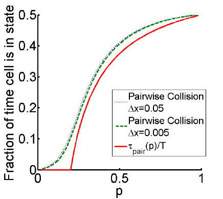
(a)

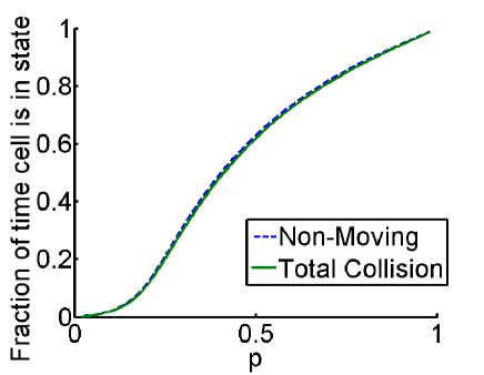
(b)

Figure 13: (a) Dependence of $\tau_{pair}(p)/T$ from MSM simulations with lattice size $\Delta x=0.05$ (dash-dotted line) and $\Delta x=0.005$ (dashed line) in comparison with the analytical expression (8) for $\tau_{pair}/T$ (solid line) where $T=8$. (b) Relative time cells spend non-moving per period $T=8$ (dashed line) vs. relative total jam time $\tau/T$ (solid line) with $\Delta x=0.005$. $\tau$ includes both indirect and pairwise collisions. Decrease of $\triangle x$ results in better match between each pairs of curves.

compares $\tau_{pair}(p)/T$ simulations obtained using MSM with simulations from (8). MSM simulations were performed with the periodic boundary conditions at the spatial interval of length $1000$ and initial random placement of $N$ cells (avoiding configurations forbidden by excluded volume principle). We used $\triangle x=0.05$ and $\triangle x=0.005$. $N$ was chosen for each simulation to match given $p$ (i.e. $N=1000\,p$). All types of collision times were calculated by running simulations till the final simulation time $t_{final}=10^{6}$. We also assumed ergodicity and recorded collisions of all cells during each such simulation. Convergence was tested by comparing the results from a subset of densities to results obtained with $t_{final}=10^{7}$ and a good match was demonstrated. Ergodicity was also tested by comparing the collision time results from several different stochastic realizations with $t_{final}=10^{6}$ and a very good match was shown for tested density values.

Figure 13a shows that MSM simulations and (8) are in a reasonably good agreement for $p>p_{0}$. For $p<p_{0}$ we generally need to modify (8) to include the fluctuations of the reversal time. Such modification is outside the scope of this paper. We however can immediately estimate the order of such modification. E.g., for $p=p_{0}$ cells do not collide without fluctuations of $T$ but they often come to zero distance between them and move in parallel as explained in Section IV. It means that if we include fluctuations of $T$ then the typical pairwise collision time will be $\sim\Delta T_{0}$. Respectively $\tau_{pair}(p_{0})$ takes a value $\tau_{pair}(p_{0})\sim\Delta T_{0}$ (in contrast with $\tau_{pair}(p_{0})=0$ in (8)) in good agreement with Figure 13a ($\Delta T_{0}/T=0.09$ for the parameters of MSM of Figure 13a while $\tau_{pair}(p_{0})/T\simeq 0.1$ for the dashed curve of Figure 13a). For $p<p_{0}$ such modification is decreased because for smaller density cells collide only due the random walk from the fluctuations of $T$. Smaller the density, more time it takes for random walk to ensure collisions. It results in the decay of $\tau_{pair}(p)$ to zero as $p\to 0.$ For $p>p_{0}$ the fluctuations of $T$ results in more efficient exploration of the space by cells which increase $\tau_{pair}$ compare with (8). This explains the difference between solid curve and dashed curve in Figure 13a.

We also performed simulations with decreasing values of $\triangle x$ to demonstrate that $\triangle x=0.05$ is already small enough to give a good approximation of $\tau_{pair}(p)$ compare with the continuous limit $\triangle x\to 0$. Figure13a shows that with dashed and dotted curves corresponding to $\tau_{pair}(p)$ for $\triangle x=0.005$ and $\triangle x=0.05$, respectively.

The same MSM simulations were used to calculate the total collision time per period $T$. In simulations we distinguish two types of the total collision time. The first type is the total collision time $\tau$ itself (total jam time per period $T$) which includes both pairwise jams and indirect jams. The second type is the average time (per period $T$) cells spend without movement which includes pairwise jams, indirect jams and jams due to finite value of $\triangle x$. The third contribution occurs when two cells are attached to each other and move in the same direction. If a cell which moves behind second one, is chosen by the MSM algorithm then its movement is prevented by the second cell. This artificial effect is due to discretization and finite value of $\triangle x$. It disappears for $\triangle x\to 0$ so that both types of the total collision time are the same in that limit. Figure 13b shows the time cells spend without movement per period $T$ versus $\tau$. It demonstrates that these total collision times (normalized to $T$) are very close to each other for $\triangle x\to 0.005$.

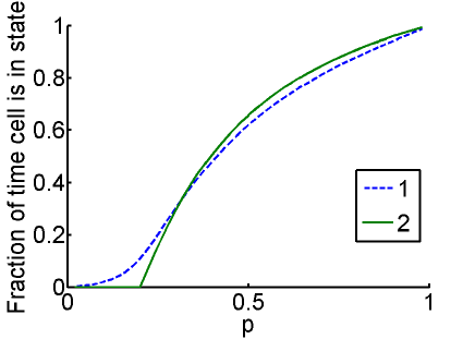
Figure 14: Plots of the total collision time per period $\tau/T$ from MSM simulations (dashed line 1) and from the analytic approximation of $\tau_{approx}$ $(\ref{tauanapprox})$ (solid line 2). The lattice size is $\triangle x=0.005$ and $T=8$.

In contrast to the pairwise collision time used in (8), the equation (7) includes an extra term $\tau O(\tau/{T})$ which corresponds to the total jam time $\tau$ per period $T$. Dashed line in Figure 14 shows $\tau(p)$ dependence in MSM simulations with the noise in $T$ (with the standard $\Delta T_{0}=0.9$). We now approximate the term $\tau O(\tau/{T})$ in the equation (7) in the simplest possible way neglecting noise in $T$ as $O(x)=c_{1}x$ with $c_{1}=2$ which yields

$$\tau_{approx}(p)=\tau_{pair}(p)\left[1+2\frac{\tau_{pair}(p)}{T}\right]\Theta(p-p_{0}),$$ (9)

where $\tau_{pair}(p)$ is given by (8). $\Theta$-function reflects the neglect of noise in $T$ similar to (8). We choose $c_{1}=2$ here to ensure correct asymptotic value $\tau_{approx}(1)=T$ for $p=1$ because all cells are jammed all the time in that case. Figure 14 shows a reasonably good fit between (9) (solid line 2) and the total collision time per period $\tau/T$ from MSM simulations with $\Delta T_{0}=0.9$ (dashed line 1). It suggests that if we add an effect of noise in (9) then it might become very good fit. Exact analytical theory is needed in order to verify this hypophysis which is quite a challenging problem and which is outside the scope of this article.

IX Conclusions and Discussion

In this paper, a connection was established between stochastic 1D model of microscopic motion of the system of regularly reversing self-propelled rod-shaped cells and a nonlinear diffusion equation describing macroscopic behavior of this system. Macroscopically (ensemble-vise) averaged stochastic dynamics was shown to be in a very good agreement with the numerical solutions of the nonlinear diffusion equation (1), where the diffusion coefficient was obtained using BM analysis. Critical density $p_{0}$ was found such that for $p<p_{0}$ the cellular diffusion is dominated by the diffusion (random walk) of individual cells while for $p>p_{0}$ the diffusion is dominated by the collisions between cells. $p_{0}$ was determined (4) from the condition that cells do not jam with each other in the no noise limit. We found that the role of noise in the reversal period is crucial. Without noise, BM analysis cannot reproduce the MSM dynamics which means that nonlinear diffusion is not a good approximation for the MSM dynamics. However, even relatively small level ($\Delta T_{0}/T\simeq 0.1$) of such noise produces excellent agreement between BM based nonlinear diffusion and MSM simulations. The primary role of such small noise is to ensure randomization of collisions between different cells in the system at large in comparison with the reversing period $T$ times.

An analytical approximation of the pairwise collision time $\tau_{pair}$ (8) and semi-analytical fit for the total jam time per reversal period $\tau_{approx}(p)$ (9) have been also obtained. Frequent collisions for $p>p_{0}$ are responsible for the nonlinear diffusion of the cellular density. For $p<p_{0}$ cells tend to spread out so their collisions are possible only if we take into account the fluctuations of the reversal time. Without such fluctuations there are no collisions and no cellular transport is possible because cells experience periodic motion in space and time. There still remains quite a challenging problem of developing a full statistical theory of 1D self-propelled rod dynamics with reversals which would be applicable for all densities. Such theory would require a detailed description of formation and interaction of large cellular clusters.

It was also shown that nonlinear diffusion coefficient $D(p)$ used to describe the macroscopic process, changes depending on the reversal period. Small and large reversal periods yield diffusion coefficients that favor high and low density diffusion respectively as is shown in Figure 7. Since dynamics of the system is determined by the dimensionless parameters $vT/L$ (the ratio of distance traveled by cells between reversals and the cell length) and $p$, increase of the speed at which cells move is equivalent to the increase of the reversal period. Thus, cell populations with small $T$ are able to spread out effectively at high densities while large $T$ promotes cell population swarming at smaller densities.

An interesting problem to be studied in future work is to determine the optimal choice of reversal time $T$ maximizing the swarming rate of Myxobacteria colony using nonlinear diffusion equation, and compare it with the one obtained in Wu09 using stochastic model.

Appendix A Boltzmann-Matano Analysis

In this appendix we review Boltzmann-Matano (BM) Analysis (see BoltzMat for details) for the readers convenience. Assume that the process we are studying can be modeled using the nonlinear diffusion equation (1) with some unknown nonlinear diffusion coefficient $D(p)$.

BM analysis allow to recover $D(p)$ from the 1D dynamics of the cellular density $p$ with the stepwise initial condition

$$p(x,0)=\begin{cases}p_{L},\quad&\text{if }\ x<x_{M}\\ p_{R}&\text{if }\ x>x_{M}\end{cases}.$$ (10)

at infinite 1D domain. Here we assume that $p_{L}>p_{R}$.

Special property of the stepwise initial condition is that it does not have any spatial scale (spatial size of system is infinite and spatial scale of jump at $x=x_{M}$ is zero. Then the only possible solution has a self-similar form $\rho(\zeta)$ which was found by Boltzmann in 1894. Here

$$\zeta=(x-x_{M})/t^{1/2}$$ (11)

which is motivated by a self-similar solution of a heat equation (for $D=const$). $x_{M}$ is a reference point also known as the Matanos interface. Assuming that $p(\zeta)$ does not depend on $t$ explicitly, we obtain that $\displaystyle\frac{\partial}{\partial t}p(\zeta)=-\frac{1}{2}\frac{\zeta}{t}\frac{\partial}{\partial{\zeta}}p(\zeta)$ and $\displaystyle\frac{\partial}{\partial x}p(\zeta)=\frac{1}{t^{1/2}}\frac{\partial}{\partial{\zeta}}p(\zeta)$ which allows to reduce (1) to

$$-\frac{\zeta}{2}\frac{\partial}{\partial{\zeta}}p=\frac{\partial}{\partial{\zeta}}\Big{[}D(p)\frac{\partial}{\partial{\zeta}}p\Big{]}.$$ (12)

Since the solutions to a non-linear diffusion equation with stepwise initial conditions are monotonic, it follows that for any given fixed time the function $p(x)$ is invertible with respect to $x$. Below we use the notation $x(p)$ for the inverse of $p(x)$. Integrating both sides of (12) with respect to $\zeta$ yields

$$-\frac{1}{2t^{1/2}}\int_{p_{L}}^{p}(x(p)-x_{M})dp=D(p)p_{\zeta}$$

where the left hand side follows from

$$\int_{-\infty}^{\zeta}\zeta\frac{\partial p}{\partial{\zeta}}d\zeta=\int_{p_{L}}^{p}\zeta(p)dp=\frac{1}{t^{1/2}}\int_{p_{L}}^{p}(x(p)-x_{M})dp.$$

Since $\frac{\partial p}{\partial\zeta}=t^{1/2}\frac{\partial p}{\partial x}$, the equation can be rewritten as

$$D(p)=-\frac{1}{2t}\left[\frac{\partial p}{\partial x}\right]^{-1}\int_{p_{L}}^{p}(x(p)-x_{M})dp,$$

which gives the Boltzmann description of the diffusion equation. Now it is possible to calculate the appropriate value of the interface, $x_{M}$, to ensure that the diffusion calculation is consistent. Specifically, since mass diffuses from the left to the right across the interface, there is a mass conservation equation where the mass lost on the left of the interface should equal the mass gained on the right of the interface,

$$\int_{-\infty}^{x_{M}}(p_{L}-p(x))dx=\int_{x_{M}}^{\infty}(p(x)-p_{R})dx.$$

Again inverting $p(x)$, we can calculate the area under of the integrals in terms of $x(p)$ to get the following equivalent expression

$$\int_{p_{M}}^{p_{L}}(x(p)-x_{M})dp=\int_{p_{R}}^{p_{M}}(x_{M}-x(p))dp,$$

which simplifies to

$$\int_{p_{L}}^{p_{R}}(x(p)-x_{M})dp=0.$$

Mass conservation occurs precisely when

$$x_{M}=\frac{\int_{p_{L}}^{p_{R}}x(p)dp}{p_{L}-p_{R}},$$ (13)

which is the Matano’s result to determine $x_{M}$ if it is unknown in advance.

In our simulations we know $x_{M}$ in advance so in fact we use Boltzmann analysis, but not BM analysis (except additional tests discussed in Appendix B). Also in our simulations $p_{L}=p_{max}$ and $p_{R}=0.$

Appendix B Accuracy of Boltzmann-Matano Analysis

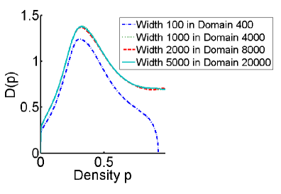
(a)

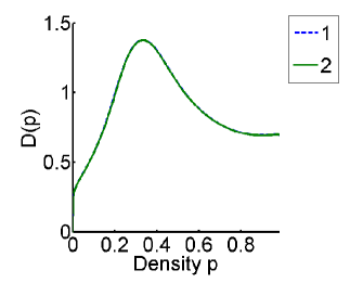
(b)

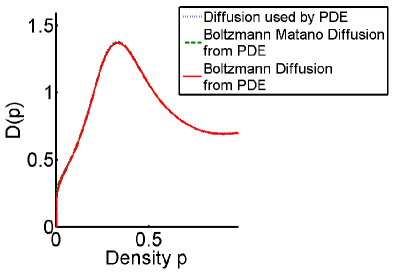
(c)

Figure 15: (a) The nonlinear diffusion coefficient $D(p)$ determined from BM analysis of MSM simulations with different initial top-hat widths. The density profiles at $t_{D}=500$ were used for all curves. It is seen that curves for the widths 1000 and above are almost undistinguishable. (b) $D(p)$ obtained from MSM simulations (dashed line - curve 1) and PDE simulation (solid line - curve 2) for top-hat initial conditions of width $600$. Density profile at time $t_{D}=1,000$ is used for BM analysis. (c) Comparison of BM analysis with Boltzmann analysis from PDE density profile at $t_{D}=500$. Dashed line is $D(p)$ used to produce density profiles from PDE simulations. All curves at (b) and (c) are almost indistinguishable.

BM analysis, described in Appendix A, is defined on infinite spatial interval with step-wise initial conditions only. Assume now that we apply BM analysis for top-hat initial conditions as described in Section II. In that case BM analysis is only approximate one because initial conditions include spatial scale $x_{width}$, which is the spatial width of top-hat. Self-similar solution of Appendix A does not agree with top-hat. That solution is only approximately valid in the neighborhood of each of two steps of top-hat. Because of spatial symmetry it is enough to consider any of these two steps. To estimate the accuracy of BM analysis in that case we note that if the density at $x=0$ (middle of top-hat) remains nearly constant then BM analysis is still applicable (except small unavoidable corrections because for any $t>0$ density is never exactly constant). Assuming that the diffusion coefficient $D(p)\sim 1$, we roughly estimate that the width of initial top-hat doubles with time when $D(p)t_{0}/x_{width}^{2}\sim 1$ which gives $t_{0}\sim 10^{6}$ for $x_{width}=1000$. For $t\ll t_{0}$ a change of density in the middle of top-hat is small in agreement with Figure 6. A similar limitation of BM analysis is that the total spatial width of the simulation domain must exceed the width of top-hat in several times to make sure that the cellular density remains low at boundaries as seen in Figure 6.

As additional test of BM analysis we varied the domain length and width of the initial top-hat distribution calculating diffusion coefficient by BM analysis from MSM simulations (Figure 15a). We observed that small top-hat width $\sim 100$ is not enough for applicability of BM analysis(dash-dotted curve in Figure 15a) while top-hat widths $\gtrsim 1000$ total domain lengths $\gtrsim 4000$ are far enough for such applicability. Figure 15b compares $D(p)$ obtained from PDE simulation (solid line) and MSM simulations (dashed line) for top-hat initial conditions of width $600$. Difference between these curves is almost indistinguishable. This indicates that our statistical ensemble in MSM simulations is large enough to avoid influence of noise in the data on the diffusion curve. We also tested MSM data with and without the Gaussian filter and obtained the same diffusion curves. Larger widths were also tested and proven to match very well, but the results are not displayed here. From these observations, we can conclude that the generated diffusion curves are independent of the width of the top hat used if the top hat is sufficiently long enough in such a way that the center and boundaries have constant density.

We would like to point out to avoid confusion that we need BM analysis only to determine the diffusion curves at reasonably small times ($t\ll t_{0}$). After that we run PDE simulations with these diffusion curves for much longer time (when density is changing both at the middle of top-hat and at boundaries). For these much larger times we also see very good agreement between MSM simulations and PDE simulations (see e.g. Figures 3 and 7).

As discussed in Section VII, another limitation of BM analysis is the loss of numerical precision near $p(x)=const$ because BM analysis requires calculating $(dp(x)/dx)^{-1}$. Many Figures (6 and 15) have jumps of $D(p)$ near $p=1$ which is due to such loss of numerical precision which can be fixed by the polynomial extrapolation. That is however not necessary because these jumps do not change results of PDE simulations in any significant way.

We also tested BM analysis vs. Boltzmann analysis as shown in Figure 15c. Although we know $x_{M}$ from top-hat initial conditions, but for finite width of top-hat we can ask if allowing $x_{M}$ to be located not exactly at the step of top-hat could improve the accuracy of BM analysis to determine $D(p).$ In that sense we can consider $x_{M}$ as additional fitting parameter to accomodate finiteness of top-had width. Figure 15c compares diffusion curves obtained from BM and Boltzmann analysis vs. exact diffusion curve. We see that difference in accuracy between BM and Boltzmann analysis is very small. It appears the advantage of using BM analysis vs. Bolztmann analysis is not significant in our case.

References

- (1) D. Kaiser, Curr. Bio. 17, 561 (2007).
- (2) Y. Wu, D. Kaiser, Y. Jiang, and M. Alber, PLoS Computational Biology 3, e253 (2007).
- (3) A. Kaiser and C. Crosby, Cell Motility 3, 227245 (1983).
- (4) R. Yu and D. Kaiser, Molecular Microbiology 63, 454 (2007).
- (5) Y. Wu, D. Kaiser, Y. Jiang, and M. Alber, Proc. Natl. Acad. Sci. USA 106, 1222 (2009).
- (6) T. Mignot, J. Merlie, and D. Zusman, Science 310, 855 (2005).
- (7) D. E. Whitworth, ed., Myxobacteria Multicellularity and Differentiation (ASM Press, 2008).
- (8) M. Alber, N. Chen, T. Glimm, and P. M. Lushnikov, Phys. Rev. E 73, 051901 (2006).
- (9) M. Alber, N. Chen, P. M. Lushnikov, and S. A. Newman, Phys. Rev. Lett. 99, 168102 (2007).
- (10) P. M. Lushnikov, N. Chen, and M. Alber, Physical Review E 78, 061904 (2008).
- (11) M. Alber, R. S. Gejji, and B. Kazmierczak, Appl. Math. Lett. 22 (2009).
- (12) C. S. Patlak, Bull. Math. Biophys. 15, 311 (1953).
- (13) E. F. Keller and L. A. Segel, J. Theor. Biol 26, 399 (1970).
- (14) M. P. Brenner, P. Constantin, L. P. Kadanoff, A. Schenkel, and S. C. Venkataramani, Nonlinearity 12, 1071 (1999), ISSN 0951-7715.
- (15) P. M. Lushnikov, Physics Letters A 374, 1678 (2010).
- (16) S. Dejak, P. Lushnikov, Y. Ovchinnikov, and I. Sigal, Submitted to Physica D (2010).
- (17) P. J. Murray, C. M. Edwards, M. J. Tindall, and P. K. Maini, Phys. Rev. E 80, 031912 (2009).
- (18) D. Gupta and T. J. Watson, Diffusion processes in advanced technological materials (Birkhäuser, 2005).
- (19) R. Welch and A. D. Kaiser, Proc. Natl. Acad. Sci. USA 98, 14907 (2001).
- (20) L. D. Landau and E. M. Lifshitz, Statistical Physics (Butterworth-Heinemann; 3rd edition, 1980).
- (21) M. Nixon and A. Aguado, Feature extraction and image processing (Academic Press, 2008).