Dusty Blastwaves of Two Young LMC Supernova Remnants: Constraints on Postshock Compression

Abstract

We present results from mid-IR spectroscopic observations of two young supernova remnants (SNRs) in the Large Magellanic Cloud (LMC) done with the Spitzer Space Telescope. We imaged SNRs B0509-67.5 and B0519-69.0 with Spitzer in 2005, and follow-up spectroscopy presented here confirms the presence of warm, shock heated dust, with no lines present in the spectrum. We use model fits to Spitzer IRS data to estimate the density of the postshock gas. Both remnants show asymmetries in the infrared images, and we interpret bright spots as places where the forward shock is running into material that is several times denser than elsewhere. The densities we infer for these objects depend on the grain composition assumed, and we explore the effects of differing grain porosity on the model fits. We also analyze archival XMM-Newton RGS spectroscopic data, where both SNRs show strong lines of both Fe and Si, coming from ejecta, as well as strong O lines, which may come from ejecta or shocked ambient medium. We use model fits to IRS spectra to predict X-ray O line strengths for various grain models and values of the shock compression ratio. For 0509-67.5, we find that compact (solid) grain models require nearly all O lines in X-ray spectra to originate in reverse-shocked ejecta. Porous dust grains would lower the strength of ejecta lines relative to those arising in the shocked ambient medium. In 0519-69.0, we find significant evidence for a higher than standard compression ratio of 12, implying efficient cosmic-ray acceleration by the blast wave. A compact grain model is favored over porous grain models. We find that the dust-to-gas mass ratio of the ambient medium is significantly lower than what is expected in the ISM.

1 Introduction

Supernova remnants (SNRs) provide a laboratory to study various aspects of interstellar medium (ISM) evolution across the whole electromagnetic spectrum. With the advent of high spatial resolution telescopes in both the X-ray and infrared (IR) regimes, it is possible to probe the interaction of the rapidly moving shock wave with the dust and gas of the surrounding ambient medium and to study the ejecta products of the SN itself. The expanding shockwave sweeps up and heats gas to $10^{6}-10^{9}$ K, causing it to shine brightly in X-rays. Dust grains embedded in the hot, shocked plasma are collisionally heated, causing them to radiate at IR wavelengths, and slowly destroying them in the process via sputtering. Because the physical processes behind X-ray and IR emission are related, a combined approach to studying SNRs using both energy ranges can reveal more information than either could on its own.

To better characterize IR emission from SNRs, we conducted an imaging survey with the Spitzer Space Telescope of $\sim 40$ known SNRs in the Large and Small Magellanic Clouds. The Clouds were chosen because of their known distance and relatively low Galactic IR background. Subsequently, we obtained IR spectra of several of the SNRs in the LMC using the Infrared Spectrograph (IRS) on Spitzer. We report here on IRS observations of two of these, SNRs B0509-67.5 (hereafter 0509) and B0519-69.0 (hereafter 0519). Both are remnants of thermonuclear SNe (Smith et al., 1991; Hughes et al., 1995) and have fast, non-radiative shocks (several thousand km s^-1) (Tuohy et al., 1982; Ghavamian et al., 2007). There is no evidence in either for slower, radiative shocks. They are both located in the LMC, at the known distance of $\sim 50$ kpc. In addition, both have ages determined from light echoes (Rest et al., 2005), with 0509 being 400 $\pm 120$ and 0519 being 600 $\pm 200$ years old. They are nearly identical in size, having an angular diameter of $\sim 30$”, which corresponds to a physical diameter of $\sim 7.3$ pc.

In Borkowski et al. (2006) hereafter Paper I, we used 24 and 70 $\mu$m imaging detections of both SNRs to put limits on the post-shock density and the amount of dust destruction that has taken place behind the shock front, as well as put a limit on the dust-to-gas mass ratio in the ambient medium, which we found to be a factor of several times lower than the standard value for the LMC of $\sim 0.25$% (Weingartner & Draine 2001, hereafter WD01). These limits, however, were based on only one IR detection, at 24 $\mu$m, with upper limits placed on the 70 $\mu$m detection. Both remnants were detected with Akari (Seok et al., 2008) at 15 and 24 $\mu$m (0519 was also detected at 11 $\mu$m). Seok et al. applied single-temperature dust models to Akari data, deriving warm dust masses of 8.7 $\times 10^{-5}$ $M_{\odot}$ and $3.6\times 10^{-4}$ $M_{\odot}$ in 0509 and 0519, respectively. With full spectroscopic data, we can place much more stringent constraints on the dust destruction and dust-to-gas mass ratio in the ISM. We also explore alternative dust models, such as porous and composite grains.

Additionally, we examine archival data from the Reflection Grating Spectrometer (RGS) onboard the XMM-Newton X-ray observatory. The high spectral resolution of RGS allows us to measure the strength of lines in X-ray spectra. We can use post-shock densities derived from IR fits to predict the strength of lines arising from shocked ambient medium, and can thus derive relative strengths of ejecta contributions to oxygen lines. Doing this requires knowledge of the shock compression ratio, $r$, defined as $n_{H}/n_{0}$ (where $n_{H}$ and $n_{0}$ are postshock and preshock hydrogen number densities, respectively), which for a standard strong shock (Mach number $\gg$ 1) is 4. However, shock dynamics will be modified (Jones & Ellison, 1991) if the shock is efficient at accelerating cosmic rays, and $r$ can be increased by a factor of several. We use several representative values of $r$ in modeling X-ray line strengths.

2 Observations and Data Reduction

We mapped both objects using the long wavelength (14-38 $\mu$m), low-resolution ($\Delta\lambda/\lambda$ 64-128) (LL) spectrometer on Spitzer’s IRS (Program ID 40604). For 0509, we stepped across the remnant in seven LL slit pointings, stepping perpendicularly 5.1^′′ each time. This step size is half the slit width, and is also the size of a pixel on the LL spectrograph. We then shifted the slit positions by 56^′′ in the parallel direction and stepped across the remnant again, ensuring redundancy for the entire object. This process was repeated for each of the two orders of the spectrograph. Each pointing consisted of two 120-second cycles, for a total observing time of 6720 s.

For 0519, the process was identical in terms of number of positions and step sizes in between mappings, but each pointing consisted of four 30-second cycles, for a total observing time of 3360 s. The difference was due to the fact that 0519 is several times brighter in the wavelength range of interest, and we did not want to saturate the detectors.

To estimate the uncertainties in the data, we fit a second-order polynomial to the line-free wavelength regions ($\sim 21-32$ $\mu$m) in the spectra where the signal-to-noise was adequate for modeling. The standard deviations of the data points in these regions were used for $\chi^{2}$ fitting of dust emission models (see Section 4.1). We obtained $\sigma$ values of 0.830 and 2.53 mJy for 0509 and 0519, respectively.

The spectra were processed at the Spitzer Science Center using version 17.1 of the IRS pipeline. We ran a clipping algorithm on the spectra which removes both hot and cold pixels that are more than 3-$\sigma$ away from the average of the surrounding pixels. To extract the spectra, we used SPICE, the Spitzer Custom Extraction tool. Once all spectra were extracted, we stacked spectra from the same spatial location, improving the signal-to-noise ratio of the sources. For background subtraction, we use the off source slit positions that come when one of the two slit orders is on the source. In the end, we have seven (overlapping) background subtracted spectra for each remnant. As we show in Section 3, this allows us to do spatially resolved spectroscopy, despite the fact that the remnants are only $\sim 30^{\prime\prime}$ in diameter.

We processed archival XMM-Newton RGS data from the XMM Science Archive with version 8.0 of the Science Analysis Subsystem (SAS) software for XMM. RGS provides high-resolution ($\Delta\lambda$ $\sim 0.04$ Å) X-Ray spectroscopy in the wavelength range from 5-38 Å. B0509-67.5 was observed on 4 July 2000 (Obs. ID 0111130201, PI M. Watson) for 36 ksec. Of these 36 ksec, only the last $\sim 2500$ s were affected by flaring. We discarded these and use the remaining 33.5 ksec for our analysis. We use the spectra from both RGS 1 and 2, and bin the data using the FTOOL grppha to a minimum of 25 counts per bin. Both RGS orders contained $\sim 8000$ counts after time-filtering. B0519-69.0 was observed on 17 September 2001 (Obs. ID 0113000501, PI J. Kaastra) for 48.4 ksec. After time filtering, we obtained $\sim 35$ ksec of useful data, with $\sim 12000$ counts in both RGS 1 and 2. We also grouped these by a minimum of 25 counts per bin. Since RGS is a slitless spectrometer, spatial information is degraded for extended sources, and the spectrum is smeared by the image of the source. In order to model RGS spectra, the response files generated by SAS must be convolved with a high-resolution X-ray image. For that purpose, we used archival broadband Chandra images from 2001 (Obs. ID 776, PI J. Hughes), along with the FTOOL rgsrmfsmooth, to produce new response matrices.

3 Results

3.1 0509

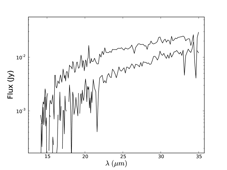
Figure 2: Top curve: Spitzer IRS spectrum of “bright” region of 0509. Bottom curve: spectrum of “faint” region. Note the differences in the slope of the spectra, in addition to the overall intensity.

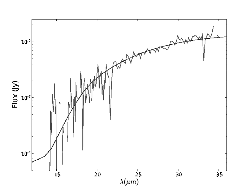
Figure 3: 14-35 $\mu$m IRS spectrum of the “faint” region of 0509, overlaid with model fit.

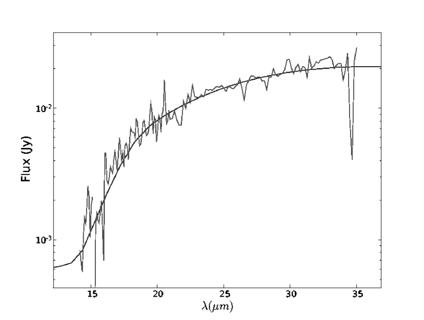
Figure 4: 14-35 $\mu$m IRS spectrum of the “bright” region of 0509, overlaid with model fit.

In the top left panel of Figure 1, we show the MIPS 24 $\mu$m image of 0509, with overlays as described in the caption. Immediately obvious is the large asymmetry in 0509, where the remnant brightens from the faint NE hemisphere to the brighter SW. Dividing the remnant in half and measuring the 24 $\mu$m fluxes from each half, we find a flux ratio of five between these two regions. At X-ray wavelengths, we measure a much more modest ratio of 1.5 from archival broadband Chandra images. Using IRS, we separated the remnant into 7 overlapping regions from which spectra were extracted. For our analysis, we chose two regions (shown on Figure 1) that do not overlap spatially and provide adequate signal to noise spectra. These regions roughly correspond to the bright and faint halves of the remnant, and the spectra are shown in Figure 2. In Figure 3 and Figure 4, we show both of these spectra separately, with models overlaid (models are discussed in Section 4). The ratio of integrated fluxes from 14-35 $\mu$m for the two regions is $\sim 2.5$. This differs from the factor of 5 measured from the photometric images because the slits are not exactly aligned with the bright and faint halves of the remnant, and because of the differences in the MIPS and IRS bandpasses.

A few obvious features immediately stand out about both spectra. First, there is no line emission at all seen in either spectrum. This is not unexpected, since the shocks in 0509 are some of the fastest SNR shocks known, at $>5000$ km s^-1 (Ghavamian et al., 2007), and there is no optical evidence for radiative shocks. Second, though both spectra show continuum from warm dust, there are obvious differences in the spectra. An inflection around 18 $\mu$m can be seen in the spectrum from the bright half, while this feature is not as clear in the faint spectrum. We attribute this feature to the Si-O-Si bending mode in amorphous silicate dust. In Section 7, we will explore reasons for the different spectral shapes and the differences in brightness between the two halves of the remnant.

3.2 0519

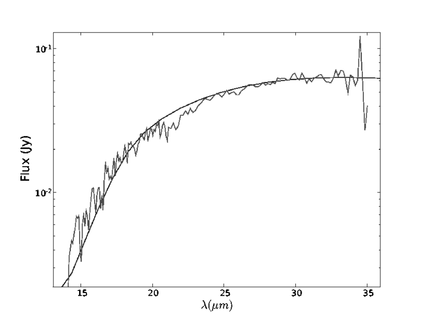
Figure 5: 14-35 $\mu$m IRS spectrum of 0519, extracted from a slit placed across the middle of the remnant, free of emission from the bright knots seen in the 24 $\mu$m image; with model overlaid.

In the bottom left panel of Figure 1, we show the 24 $\mu$m image of 0519, which does not show the large scale asymmetries that 0509 does, although three bright knots can be seen in the image. These same three knots can be identified in both H$\alpha$ (Smith et al., 1991) and X-ray images, where Chandra broadband data shows that the three knots are prominent in the 0.3-0.7 keV band (Kosenko et al., 2010). In Paper I, we measured the total flux from the three knots added together and found that collectively they represent only about 20% of the flux. Nevertheless, spectra extracted from slits that contain a bright knot do show differences in continuum slope from those extracted where no knots are present. We discuss our interpretation of these knots in Section 7. As with 0509, there are no lines seen in the IRS data (see Figure 5), as shock speeds are also quite high in this object.

4 IRS Fits

We now turn our attention to modeling the emission seen in IRS with numerical models of collisionally heated dust grains. We follow a procedure identical to that followed in our previous work on these objects; see Paper I. The heating rate of a dust grain immersed in a hot plasma depends on both the gas density (collision rate) and gas temperature (energy per collision). In general, the electron temperature of a shocked plasma can be determined from fits to X-ray spectra. In the case of these objects, plane-shock models without collisionless heating of electrons at the shock front yield the temperature. Dust heating models do depend on this temperature, but the dependency is not large (Dwek, 1987). Gas density is a much more sensitive parameter for dust heating models, and is determined by the temperature of the grains. We regard postshock gas density as a free parameter in our model, and fine tune the density to match the observed IR spectra.

We take into account sputtering by ions, which destroys small grains and sputters material off large grains. We use a plane-shock model which superimposes regions of increasing shock age (or sputtering timescale) $\tau_{p}=\int_{0}^{t}n_{p}dt$, where $n_{p}$ is post-shock proton density, while keeping temperature behind the shock constant. Inputs to the model are an assumed pre-shock grain-size distribution, grain type and abundance, proton and electron density, ion and electron temperature. The code calculates the heating and sputtering for grains from 1 nm to 1 $\mu$m, producing a grain temperature and spectrum for each grain size. The spectra are then added in proper proportions according to the post-sputtering size distribution to produce a model spectrum that can be compared with observations. We use sputtering rates from Nozawa et al. (2006) with enhancements for small grains from Jurac et al. (1998). We assume that sputtering yields are proportional to the amount of energy deposited by incoming particles, accounting for partial transparency of grains to protons and alpha particles at high energies (Serra Dìaz-Cano & Jones, 2008), particularly relevant for 0509 and 0519. We assume that grains are compact spheres, but we also report results and implications if grains are porous (i.e. contain a nonzero volume filling fraction of vacuum).

In general, our method is to fix as many of the input parameters as possible, based on what is known from other observations. For instance, Rest et al. (2005) used optical light echoes to constrain the ages of both remnants, yielding ages of $\sim 400$ yrs. for 0509 and $\sim 600$ yrs. for 0519. Shock velocities are known approximately for both objects from measurements of ion temperatures (Tuohy et al., 1982; Ghavamian et al., 2007). In 0509, the standard shock jump conditions for a 7000 km s^-1 shock, the assumed speed for the NE half of the remnant (Ghavamian et al., 2007) with no ion-electron equilibration would produce proton temperatures of $\sim 115$ keV. Recently, Helder et al. (2010) used VLT spectroscopy to detect a broad H$\alpha$ component from the rim of 0509, determining the shock speed to be $\sim 6000$ km s^-1 in the NE. They give several possibilities for the proton temperature in the NE, and note that energy from escaping cosmic-rays limits the post-shock proton temperature to a value of $<$ 0.85 of that expected from the strong shock jump conditions. Adopting this value of 0.85, along with a shock speed of 6000 km s^-1 and no electron heating gives a post-shock proton temperature of $<$70 keV. We use this value as an input to dust heating models, except where noted otherwise (see Section 7.2). This upper limit on proton temperature makes any fit to the density for 0509 a lower limit, and we discuss the effects of changing the proton temperature in Section 7.2.

The shock speed in 0519 is a bit more uncertain. Ghavamian et al. (2007) quote a range of 2600-4500 km s^-1 between the limits of minimal and full ion-electron equilibration. Kosenko et al. (2010) measured line widths of X-ray iron lines seen in XMM-Newton RGS spectra to obtain a velocity of 2927 km s^-1. We adopt a value of 3000 km s^-1 for this work and use the standard shock jump proton temperature assuming no electron-ion equilibration, which is 21 keV. The actual proton temperature may differ from this estimate, but the fitting of dust spectra in the IR is only weakly dependent on the proton temperature (see Section 7.2).

The overall normalization of the model to the data (combined with the known distance to the LMC) provides the mass in dust. Since our models calculate the amount of sputtering that takes place in the shock, we can then determine the amount of dust present in the pre-shock undisturbed ISM that has been encountered by the blast wave. While we are sensitive only to “warm” dust, and could in principle be underestimating the mass in dust if a large percentage of it is too cold to radiate at IRS wavelengths, it is difficult to imagine a scenario where any significant amount of dust goes unheated by such hot gas behind the high-velocity shocks present in both remnants, particularly given the upper limits at 70 $\mu$m reported in Borkowski et al. (2006) (and the fact that there are no radiative shocks observed anywhere in these remnants).

4.1 Model Uncertainties

The only fitted parameters in the model are the post-shock proton number density, which affects the shape of the model spectrum, and the radiating dust mass, which affects the overall normalization. All other variable parameters (e.g. electron density, sputtering timescale) depend directly on the density. We use an optimization algorithm to minimize the value of $\chi^{2}$ in the regions of the spectra with high signal-to-noise (for both remnants, $\sim 21-32$ $\mu$m) to find the best-fitting value of the density. We then calculate upper and lower limits on the fitted density as the 90% confidence intervals in $\chi^{2}$ space (where confidence intervals correspond to $\chi^{2}_{min}$ + 2.71), using the standard deviations listed in Section 2. The errors on both the density and dust mass present are of order 25% for 0509 and 10% for 0519. Larger errors in 0509 are due to a poorer signal-to-noise ratio in the spectrum. We assume that the plasma temperature is fixed at the values listed above, but again note that the dependency on proton and electron temperature is small (see Section 7.2).

There are also several sources of uncertainty in modeling emission from warm dust grains that are hard to quantify statistically. First and foremost, we are limited by both the spatial resolution of Spitzer for such small SNRs and the low signal-to-noise ratio of the spectra. We use a plane-shock model with constant plasma temperature to model dust emission, which is only an approximation to a spherical blast wave. Estimates of swept gas mass assume constant ambient density ahead of the shock. Sputtering rates for such high temperature protons and alpha particles are probably only accurate to within a factor of 2 (but see Appendix A), and we use the simple approximation that the sputtering rate varies according to the amount of energy deposited into a grain of given size and composition. Lastly, but possibly most importantly, we do not know the degree of porosity and mixing of various grain types.

4.2 IR Morphologies

Although we have full spectral mapping of both objects, the 10.5^′′ width of the IRS slit severely limits the amount of spatially resolved spectroscopy we can do on remnants that are only 30^′′ in diameter, as both 0509 and 0519 are. Despite this, we do have several disjoint slit positions which isolate spectra from the most prominent features in the images. Because dust radiates as a modified blackbody spectrum, emission from a small amount of warmer dust can overwhelm that from a larger amount of colder dust, particularly at the wavelengths of interest here. We show in Figure 3 and Figure 4 spectra extracted from two regions of 0509, which we label the “faint” and “bright” portions of the remnant. Fits to these regions require a density contrast of $\sim 4$ in the post-shock gas, with the higher density required in the “bright” region (higher densities means hotter dust, hence more short wavelength emission). Although it might be possible that a density gradient of this order actually exists in the ambient medium surrounding 0509 (the angular size of 30^′′ in the LMC corresponds to a linear diameter of about 7 pc), the implications from this model lead to several scenarios which are unlikely and require an appeal to special circumstances.

In comparing the MIPS image with images of the remnant at other wavelengths, one can clearly see an enhancement in the Chandra broadband image (Warren & Hughes, 2004) on the southwest side of the remnant. This enhancement is mostly present in the energy range containing Fe L-shell emission lines. The H$\alpha$ image, shown in Figure 1, shows a uniform periphery around the remnant, with the exception of a brightness enhancement in the SW, relatively well confined to a small region. To compare the images, we convolved the H$\alpha$ image to the resolution of the 24 $\mu$m image using the MIPS 24 $\mu$m PSF. The result is shown in Figure 6. The images are morphologically similar, and from these comparisons we conclude that there is not an overall NE-SW density gradient in the ISM. Rather, the ISM is mostly uniform except for the SW, where the remnant is running into a localized region of higher density. To obtain the conditions for the whole of the remnant, we fit a model to the “faint” region, freezing all parameters to those reported in Table 1 and allowing post-shock density to vary (which also causes the sputtering timescale to vary). If we assume a standard LMC dust model (Weingartner & Draine, 2001), we get a post-shock density of $n_{H}$ = 0.59 cm^-3. The reduced $\chi^{2}$ value for this model was 1.04. Values in Table 2 correspond to this “faint” region.

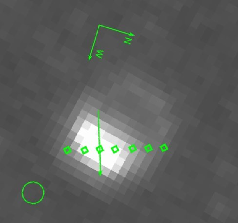
Figure 7: 24 $\mu$m image of 0509. Arrow shows both direction of slit placement and length of inferred brightness enhancement in that spatial direction. Diamonds are extraction centers for the parallel slit positions extracted in the text (note that arrow coincides with position 3). Intensity function plotted in Figure 8 corresponds to diamonds from left-to-right in this image. Green circle is MIPS 24$\mu$m PSF.

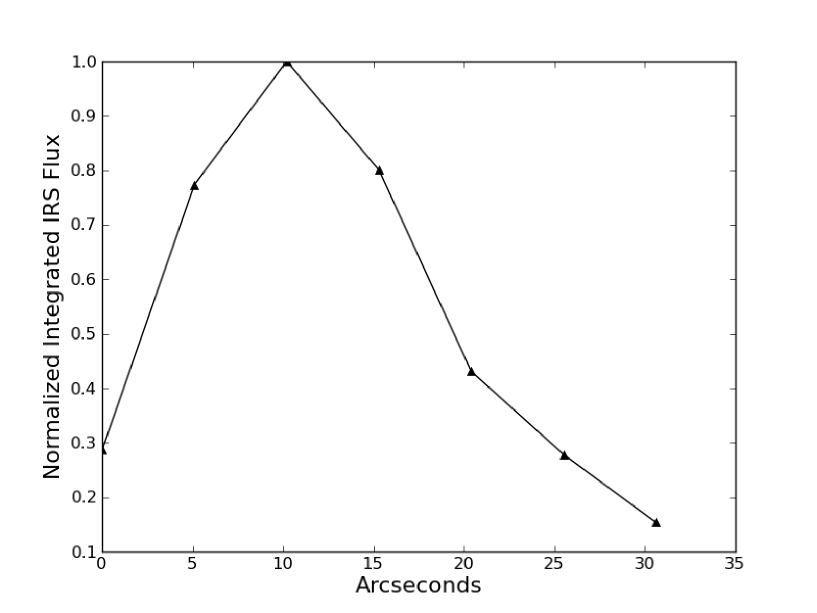
Figure 8: Intensity of background-subtracted integrated IRS flux as a function of distance from the left-most to the right-most diamond point in Figure 7.

We can use IRS to estimate the spatial extent of the bright region. First, by looking at the 2-D spectra from the LL slit located directly on top of the brightest region in the MIPS 24 $\mu$m image, we fit a gaussian to the spatial profile (indicated by an arrow in Figure 7) of the emission between 16 and 17 $\mu$m, and found a FWHM of the brightness profile of 12.7”. This wavelength is the shortest at which we could achieve a good signal-to-noise ratio for this region. The Spitzer resolution at 16 $\mu$m is about 4.75”. In the direction perpendicular to the slit positions, we had 7 slit pointings, each separated by 5.1”. Extracting spectra from each of these (overlapping) positions, subtracting the background, and integrating over the IRS bandpass gave us 7 measurements of the brightness as a function of position. The locations from which these spectra were extracted are shown as diamonds in Figure 7, and the resulting normalized intensity function is shown in Figure 8. The brightness peaks at position 3, the position we used to examine 2-D spectra, as described above, and falls off relatively quickly on both sides away from that position.

Our assumption that the bright region of 0509 is the result of a more localized enhancement in density implies that the spectrum extracted from that region is then a composite of emission from the uniform parts of the remnant and from the small, denser region. Spitzer does not have the resolution required to isolate this dense region, but we can make a crude isolation by assuming that the two slit positions in Figure 1 cover an equal surface area on the remnant, and subtracting the faint spectrum from the bright. The residual spectrum is of less than ideal signal-to-noise. Nevertheless, a fit to this spectrum implies a gas density of $\sim 6.4$ cm^-3, or about an order of magnitude higher than the rest of the remnant. A small region of hot dust outshines a more massive region of cooler dust at 24 $\mu$m, which would explain the factor of 5 ratio in the flux between the two sides. X-rays from this object are dominated by ejecta, not swept-up ISM, and there are several factors to consider beyond density when considering the flux of H$\alpha$ coming from a region. Higher resolution observations at all wavelengths will shine more light on this issue.

For 0519 we have a similar scenario, except that instead of one bright region, we have three bright knots. As noted previously, these knots correspond spatially with knots seen in both X-rays and H$\alpha$ (see Figure 1). We adopt an identical strategy here, isolating spectra from slit positions that do not overlap with one of the bright knots. As it turns out, there is only one slit position in this object that is nearly completely free of emission from a knot, a slit position that goes directly across the middle of the remnant. The spectrum from this region is shown in Figure 5. We assume that the conditions within this slit position are indicative of the remnant as a whole. Using parameters found in Table 1, we obtain a post-shock density of $n_{H}$ = 6.2 cm^-3 (reduced $\chi^{2}$ = 1.13). We do not have adequate signal-to-noise to isolate the bright knots individually. However, we approximate the density required by noting that a fit to the spectrum extracted from the entire slit position that contains the brightest of the three knots (the northernmost knot) requires a density that is higher by a factor of $\sim 2$. Given that this spectrum contains emission from both the uniform parts of the remnant and the bright knot, it is likely that the density in the knot itself is perhaps a factor of $\sim 3$ higher that the more uniform parts of the remnant, which is roughly consistent with our results from Paper I.

5 Dust Grain Porosity

While it is typically assumed in dust grain models that grains are solid bodies composed of various materials, this is likely not a physically valid model (see Shen et al. (2008), and references therein). It is possible to relax the assumption that grains are compact spheres with a filling fraction of unity. We have updated dust models to include the porosity of dust grains (where porosity, $\cal P$, is the fraction of the grain volume that is composed of vacuum, instead of grain material), as well as allowing for grains to be composite in nature, i.e. a grain made up of silicates, graphite, amorphous carbon, and vacuum. The details of this model are discussed in Williams (2010). We summarize here the important results. Perhaps the most significant effect of introducing porosity to grains is that the grain volume per unit mass increases, since the overall density of the grain is lowered. As a result, grains are more efficient radiators of energy, and less dust mass in total is required to reproduce an observed IR luminosity.

For a grain of the same mass, the grain is heated to a higher temperature if it is solid than if it is porous. As a result of the equilibrium temperature being lower for porous grains, more heating is necessary to fit the same spectrum with a porous grain model than a solid grain model. For a fixed plasma temperature, this can only be achieved by increasing the post-shock density. In summary, increasing the porosity of grains has the dual effects of raising the necessary postshock density required to heat grains to an observed temperature, while lowering the total amount of dust required to reproduce an observed luminosity.

What remains is to choose a grain “recipe” to use to fit the data. Since there are few constraints from the ISM at this time, we have adopted here two values of $\cal P$, 25 and 50%, to explore the effects of grain porosity of fitting IR data. Our “compact” model, which we used to derive results given above, assumes separate populations of solid silicate and graphite grains with appropriate size distributions for the LMC (WD01). Our “porous” grain models are based on those of Clayton et al. (2003). For the 25% porous model, we assume that grains are composed of 25% vacuum, 50% silicate, and 25% amorphous carbon. The 50% porous grains contain 50% vacuum, 33.5% silicate, and 16.5% amorphous carbon, distributed from 0.0025 to 1.5 $\mu$m. The narrow bandwidth of the IRS data does not allow us to determine which model fits the data better, as we obtained equally good fits from all models (albeit with a different value of density), and report results from all. A caveat to using these porous grain distributions is that both of them were optimized for the Galaxy, and not the LMC. However, to the best of our knowledge, a size distribution appropriate for porous grains in the LMC has not yet been developed.

The results are as follows: For 0509, the best-fit $\cal P$ = 25% model had a post-shock density, $n_{H}$, of 1.1 cm^-3 ($\chi^{2}$ = 1.05), while the $\cal P$ = 50% model required an $n_{H}$ of 2.2 cm^-3 ($\chi^{2}$ = 1.07). For 0519, the best-fit densities were 9.5 ($\chi^{2}$ = 1.08) and 17 ($\chi^{2}$ = 1.07) cm^-3 for $\cal P$ = 25 and 50%, respectively. In all cases, we assume LMC abundances, such that $n_{e}$ = 1.2$n_{H}$.

6 X-ray Modeling of RGS Data

Although dust models in the IR are a powerful diagnostic of the post-shock gas, they are insensitive to pre-shock gas conditions, which determine the total swept mass. Unlike many SNRs, both of these objects have relatively well-defined ages and distances. The post-shock densities are related to the pre-shock values by $r$, which is 4 in the case of an unmodified, strong shock, but may be greater than 4 in the case of cosmic-ray modification of the blast wave. For a given $r$, we can calculate the pre-shock density, and thus the total amount of swept up material. The product of post-shock electron density and total gas mass overrun by the blast wave is proportional to the emission measure (EM) of the X-ray emitting plasma. When combined with the ionization timescale ($\tau_{i}=\int_{0}^{t}n_{e}dt$) and electron temperature of the gas, we have all the information necessary to generate a model X-ray spectrum for the shocked ambient medium, which we can compare directly to observed X-ray spectra.

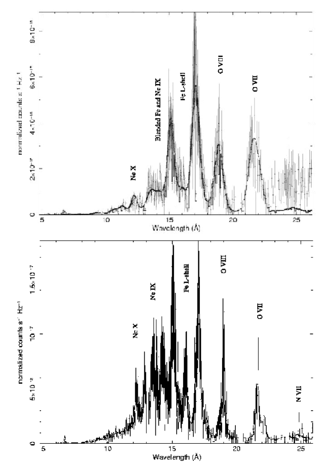
Figure 9: Top: XMM-Newton RGS spectrum of B0509-67.5, from 5-27 Å, with model overlaid as described in text. Lines of interest are marked. High shock speeds and ejecta velocities lead to significant blending of Ne lines with numerous Fe L-shell lines. Data beyond 23 Å was excluded from model fitting, and is shown only for ease of comparison with bottom panel. Bottom: Same, but for B0519-69.0. Slower speeds allow separation of Ne and Fe L-shell lines in this remnant.

The difficulty in this approach lies in disentangling X-ray emission from the shocked ambient medium from that arising from reverse-shocked ejecta. For large remnants, this could be done spatially using CCD spectra, but both 0509 and 0519 are $\sim 30^{\prime\prime}$ in diameter with the ejecta not well separated from the shocked ISM, rendering such an approach impossible. For 0509, previous studies (Warren & Hughes, 2004; Badenes et al., 2008) have used Chandra CCD spectra to model emission from the remnant, but these studies are subject to the inherent difficulty in using poor spectral resolution CCD spectra to disentangle ISM and ejecta emission. An alternative approach is to take high-resolution spectra from grating spectrometers, such as RGS on XMM-Newton. If lines can be identified as arising only from shocked ambient medium, then model fits to these lines could be directly compared with predicted line strengths from the model described above. This can be most easily done with N lines, as virtually no N is produced in Type Ia explosions. Kosenko et al. (2008) fit the 24.8 Å N Ly-$\alpha$ line in the spectrum of 0509, but we find that this line is very weak and unconstraining to the fitting procedure used here. Here we generate model O Ly$\alpha$ and K$\alpha$ lines visible in RGS spectra and compare them directly to observed line fluxes. In Figure 9, we show RGS spectra from both remnants.

6.1 0509

As seen in Figure 9, Fe L-shell lines dominate the spectrum of 0509, but strong lines from both H and He-like O are clearly visible in both cases at 18.97 and 21.7 Å. In order to measure the strength of observed O lines, we fit the data with a two-component model. One model, a vpshock model containing only iron, was fit to the data between 14-18 Å, which are dominated by iron lines. We then added a second vpshock model at fixed normal LMC abundances (wilms abundance model in XSPEC (Wilms et al., 2000), with abundances of heavy elements set to 0.4; except that N = 0.1) with ionization timescale and normalization free to fit the data between 9-14 and 18-23 Å, regions where the signal-to-noise was good enough to constrain the fit. We use two absorption components, one resulting from Galactic absorption with column density, $N_{H}$, equal to 5 $\times$ 10²⁰ cm^-2 (Staveley-Smith et al., 2003), and one from the LMC (at fixed LMC abundances; same as above), equal to 2 $\times$ 10²⁰ cm^-2 (Warren & Hughes, 2004). These models were used only to determine the strength and width of oxygen lines.

We freeze the electron temperature for the second vpshock model to 2 keV. This is roughly the number one gets from models of Coulomb heating of electrons behind a shock of 7000 km s^-1 with a preshock density of 0.25 cm^-3. Although we do not know the preshock density a priori, we use this as a representative value and note that the dependence of the emission measure of the gas on the electron temperature is small. We introduce an additional line smoothing parameter to both models to allow for the fact that lines are broadened by Doppler motions. For this model, we find that oxygen line fluxes measured from RGS spectra in 0509 are as follows: O Ly$\alpha$ = 4.41 $\times 10^{-13}$ ergs cm^-2 s^-1 and O K$\alpha$ = 5.05 $\times 10^{-13}$ ergs cm^-2 s^-1. The oxygen line widths obtained from fitting are $v_{FWHM}$ = 12350 (11220, 13630) km s^-1. Kosenko et al. (2008) measured the widths of Fe lines in the RGS spectrum of this object, obtaining line widths of 11500 (10500, 12500) km s^-1.

6.2 0519

Our technique for fitting RGS data from 0519 was identical, except that we extended the fitting range out to 27 Å to account for the fact that we had better signal-to-noise at long wavelengths in this case. We again used two absorption components; one for the galaxy with $N_{H}$ = 6 $\times$ 10²⁰ cm^-2 (Staveley-Smith et al., 2003) and one for the LMC with $N_{H}$ = 1.6 $\times$ 10²¹ cm^-2 (Hughes et al., 1995; Kosenko et al., 2010). Measured line strengths for this remnant are 5.81 $\times 10^{-13}$ ergs cm^-2 s^-1 and 3.91 $\times 10^{-13}$ ergs cm^-2 s^-1 for O Ly$\alpha$ and O K$\alpha$, respectively. We obtain a line width for oxygen lines of $v_{FWHM}$ = 3470 (3170, 4000) km s^-1. Using a three-component NEI model, Kosenko et al. (2010) measure Fe line widths in this object to be 4400 (4280, 4520) km s^-1. The also report that neither Ne nor Mg is required to fit the XMM spectra. We find that normal abundances of Ne and Mg from the shocked ISM are allowed by the data, and it is not necessary to exclude them from the fitting procedure.

Oxygen line widths in 0519 are comparable to the assumed shock velocity, while those in 0509 are significantly higher. In Section 7.3, we discuss hydrodynamic modeling of 0519, and find that given the age of 0519, a lower shock speed of 2450 km s^-1 is preferred to match the observed radius of the forward shock. Line widths from a shock of this speed would fall within errors of the observed line widths above.

7 Discussion

IR spectral fitting gives us a postshock density, which we can then divide by $r$ of the shock to get the preshock density. For a standard, “strong” shock, $r$ is $\rho_{1}/\rho_{0}=4$, but modification of shocks by cosmic ray acceleration will increase this. An additional complication for the cases of these two objects is that they are both only 30^′′ in diameter, which is quite small for the telescope resolution at Spitzer wavelengths, meaning that the spectra shown in Figures 2-4 are the average spectra over the entire postshock region. To account for this, we computed hydrodynamic models (see Section 7.3) and calculated the mean, EM-weighted $r$ over the post-shock region from the leading edge of the blast wave to the contact discontinuity. For the case of a standard shock, this mean $r$ is 2.65. This is lower than the immediate postshock value of 4 due to the sphericity of the blast wave. The postshock density drops behind a spherical shock.

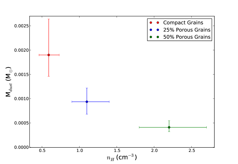
Figure 10: Best fit values for 0509 of post-shock density and dust mass, with errors, for various grain models. Errors are 90% confidence limits, as described in the text.

Taking the example of 0509, dust model fits to IR spectra give a postshock density of $n_{H}=0.59$ cm^-3. Dividing this by 2.65, we get an ambient pre-shock density, $n_{0}$, of 0.22 cm^-3. The known distance to the LMC of 50 kpc, combined with the measured angular size of the remnants, gives a shocked volume of 5.7 $\times 10^{57}$ cm³. Multiplying the pre-shock density by the volume gives the value reported in table 2 for the swept-gas mass, 1.47 $M_{\odot}$. Dividing the dust mass inferred from fits to IR data, 1.9 $\times 10^{-3}$ $M_{\odot}$, by this number, we arrive at an ambient dust-to-gas mass ratio of 1.3 $\times 10^{-3}$, the number we report in Table 1. This dust-to-gas ratio is not folded into the models at any point, nor is it ever assumed. We repeat these steps for various values of $r$, determining different swept gas masses and dust-to-gas mass ratios. However, note that the post-shock density and total dust mass remain constant for each case, since those were determined from fits to IR data. We include effects of sputtering of dust grains by ions in deriving the dust masses above. In Figures 10 and 11, we show the best fit values of post-shock density and dust mass for various grain models.

X-rays in 0509 and 0519 are coming mostly from reverse-shocked ejecta. The shocked ambient medium may contribute substantially, particularly to continua and O lines, though it is difficult to evaluate this contribution based solely on X-ray data. However, because fits to IR data provide us with the post-shock density, and the ages and sizes of these remnants are well-known, we can use X-ray emission codes to predict line strengths coming from the shocked ambient medium, assuming typical LMC abundances.

In Tables 2 & 3, we show predicted oxygen line strengths as a function of $r$ and grain porosity for both remnants. These line strengths were calculated in XSPEC by taking the plane-shock models as described in the section above and varying the ionization timescale and emission measure appropriately for each case. Real ages of 400 and 600 years for 0509 and 0519, respectively, were divided by 3 in calculating $\tau_{i}$ as a correction factor for applying a plane-shock model to a spherical blast wave (Borkowski et al., 2001). EM was calculated as $n_{e}n_{0}V$, where $n_{e}$ is post-shock electron density, $n_{0}$ is pre-shock density ($\equiv$ $\frac{n_{H}}{r}$, where V is total volume enclosed by the blast wave (approx. $5.7\times 10^{57}$ cm³ for both remnants). We chose values for $r$ of 4, 8, and 12, which correspond to mean EM-weighted $r$ values of 2.65, 4.8, and 6.8.

In the Tables, we quote our predicted O line strengths from the blast wave as a fraction of the observed strengths from RGS spectra. Values $<$ 1 imply a contribution to O lines from ejecta, while values $>$ 1 are inconsistent with observations and are ruled out. For 0519, this rules out all models of porous grains. However, this requirement also rules out compact grain models that are unmodified from “standard” shock jump conditions. Only those shocks with significantly higher $r$ are possible based on X-ray line strengths observed.

For 0509, only one case is ruled out, that of highly porous ($\cal P$ = 50%) grains heated behind a shock with standard jump conditions. If grains are compact, then virtually all O line emission seen in RGS spectra would have to come from ejecta. Recent near-IR observations of Type Ia SNe (Marion et al., 2009) suggest that the entire progenitor is burned in the explosion and that O and Ne are byproducts of carbon burning, meaning that strong X-ray lines from oxygen in the ejecta may be unlikely. The favored explosion model for 0509 from Badenes et al. (2008) contains 0.04 $M_{\odot}$ of unburned oxygen, the least of any of the explosion models considered for this remnant. Nevertheless, even this relatively small amount of ejecta oxygen could be enough to produce observed O lines. Model line ratios require at least some contribution from reverse-shocked ejecta to account for observed O Ly$\alpha$ strength.

Helder et al. (2010) find that at least some of the energy of the shock in 0509 must be deposited into cosmic rays. Of course, if cosmic-ray pressure is indeed non-negligible, then the standard case no longer applies, and cosmic-ray modified shocks would be required. Our assumed proton temperature of 70 keV already implies modification from the standard shock jump conditions, which would predict $kT_{p}$ $\sim 115$ keV. However, the dependency of the dust heating models on this number is small (see Section 7.2). The relationship between cosmic-ray pressure and shock compression ratio is model dependent (Vink et al., 2010) and beyond the scope of this paper, but models in Table 1 with $r>4$ would be preferred.

The data do not allow us to firmly distinguish between compact and porous grain fits, as both can be consistent with the data under the right circumstances. Instead, we summarize implications for each model. If dust grains in the ISM are compact, the oxygen lines visible in X-ray spectra of 0509 are dominated by contributions from the ejecta, for all values of $r$. The inferred preshock density is inversely proportional to $r$ (see Table 2). A “standard” $r$ value of 4 yields a preshock density of $n_{0}$ = 0.22 cm^-3, significantly higher than either the value of 0.05 cm^-3 quoted by Warren & Hughes (2004) or that of 0.02 cm^-3 from Tuohy et al. (1982), but below the 0.43 cm^-3 of Badenes et al. (2008). In 0519, it is possible for nearly all of O lines to be coming from shocked ambient medium; however, the minimum $r$ value required to match the O K$\alpha$ line strength observed is 12. For this value of $r$, a small ejecta contribution to the O Ly$\alpha$ line is still necessary for line ratios to match.

If grains are porous, a lower ejecta contribution to oxygen lines observed in 0509 would be permitted, even for values of $r$ that are closer to the standard shock value. However, in 0519, much higher $r$ values would be required to bring model oxygen line fluxes down to observed levels, even with no contribution from the ejecta. We require significantly less oxygen in the ejecta than Kosenko et al. (2010), who report an O ejecta mass of 0.2-0.3 $M_{\odot}$. Minimum values for $r$ would be 20 and 34 for $\cal P$ = 25% and 50%, respectively.

7.1 Radio Limits on Compression Ratio

We can set an upper limit to $r$ using the observed diffuse synchrotron brightness of the LMC near 0509 and 0519, and requiring that the brightening by compression of the ambient synchrotron emissivity not exceed the observed radio brightnesses of 0509 and 0519. Compression will boost the energy of electrons and also increase the mean magnetic field strength in the emissivity $j_{\nu}$. If the electron energy distribution is $N(E)=KE^{-s}$ between energies $E_{l}$ and $E_{h}$, then the emissivity is given by

$$j_{\nu}=c_{j}(\alpha)KB^{1+\alpha}\nu^{-\alpha}$$ (1)

where $\alpha\equiv(s-1)/2$ and $c_{j}(0.5)=4.85\times 10^{-14}$ cgs. (In general, $c_{j}\equiv c_{5}(\alpha)(2c_{1})^{\alpha}$ in the notation of Pacholczyk [1970], with $c_{1}\equiv 1.82\times 10^{18}$ and $c_{5}(0.5)=1.37\times 10^{-23}$.) Taking $\alpha=0.5$ $(s=2)$ for simplicity, we find that the electron energy density $u_{e}$ obeys

$$u_{e}\equiv\int_{E_{l}}^{E_{h}}KE^{-s}EdE=K\ln\left({E_{h}\over E_{l}}\right)\propto p_{e}\propto\rho_{e}^{4/3}\propto r^{4/3}.$$ (2)

In the absence of turbulent effects and magnetic-field amplification,the tangential component of $B$ will be increased by $r$ while the radial component will remain the same, raising the magnitude of $B$ by a factor $r_{B}<r$. For a spherical remnant encountering a uniform magnetic field, it is straightforward to show that the mean amplification factor $\langle{r_{B}\rangle}$ is $0.79r$ for $r\geq 6$. Thus, after compression, the synchrotron emissivity interior to the remnant is given by

$${j_{\nu}({\rm in})\over j_{\nu}({\rm out})}=r^{4/3}(0.79r)^{1.5}=0.70r^{17/6}.$$ (3)

For a mean diffuse surface brightness upstream of $\Sigma_{0}$ W m^-2 sr^-1, the mean emissivity in the LMC just depends on the line-of-sight depth of synchrotron-emitting material in the LMC. Calling that quantity $l$, we have $\langle{j_{\nu}({\rm up})\rangle}=\Sigma_{0}/l$. Compressing this as above predicts the post-shock surface brightness for a SNR of radius $R$, $I_{\rm SNR}$, to be about

$$I_{\rm SNR}=j_{\nu}({\rm in})R=0.70r^{17/6}j_{\nu}({\rm out})R=0.70r^{17/6}\left(\Sigma_{0}\over l\right)R$$ (4)

$$\Rightarrow r_{\rm max}=1.13\left(I_{\rm SNR}\over\Sigma_{0}\right)^{6/17}\left(l\over R\right)^{6/17}.$$ (5)

The diffuse radio brightness of the LMC has been mapped with ATCA and Parkes (Hughes et al. 2007). From the image at 20 cm (resolution $40^{\prime\prime}$), we estimate surface brightnesses near 0509 and 0519 of about 1 and 2 mJy/beam respectively, or about $1\times 10^{-21}$ and $2\times 10^{-21}$ W m^-2 sr^-1 at 1 GHz, respectively (using a mean spectral index of the diffuse emission of 0.3; Hughes et al. 2007). We take $l\sim 1$ kpc.

For 0519, a high-resolution image is available (Dickel & Milne, 1995), which shows a shell peak brightness of about 6 mJy/beam at 20 cm, giving (for $\alpha=0.5$ and a FWHM of $4.8^{\prime\prime}$) $I_{\rm SNR}\sim 1\times 10^{-19}$ W m^-2 sr^-1, and $r_{\rm max}\sim 26$. There is no high-resolution image of 0509 available; using the mean remnant surface brightness ($\sim 5\times 10^{-20}$ W m^-2 sr^-1 from data in Mills et al. 1984) slightly overestimates $r_{\rm max}$, but gives a value of 25. Larger values of $r$ would give higher radio brightnesses than we observe.

7.2 Effect of Decreased Ion Temperature on IR Fitting

If shocks are indeed modified by cosmic-ray accleration, both $r$ and the plasma temperature behind the shock would be altered from the standard strong shock jump conditions (Jones & Ellison, 1991). Helder et al. (2010) report evidence in 0509 for decreased proton temperatures due to cosmic-ray modification of the shock. In this work, we find that higher than normal values of $r$ are also necessary to avoid overpredicting oxygen lines in the X-ray spectra of 0519; such a modification would likewise lower proton temperatures from the value assumed. Dust model fits to IR data are dependent only on these post-shock conditions, and are insensitive to the degree of modification at the shock. A detailed examination of this relationship is beyond the scope of this paper, but we can make some general comments about the effect that lowering the proton temperature behind the shock would have on fitting the data. In the case of most SNRs, heating of grains by protons can be neglected, as heating is dominated by collisions with electrons. However, for remnants with very fast shocks, proton heating becomes non-negligible (Williams, 2010).

In Table 2, we use a proton temperature of 70 keV for modeling 0509. We take the case of 25% porous grains as an example (where $n_{H}$ was fit to be 1.1 cm^-3). Raising the proton temperature by a factor of $\sim 50\%$ to 115 keV, the temperature expected from a 7000 km s^-1 shock with no electron-ion equilibration lowers the fitted density to 1.0 cm^-3, an effect of only about 10%. Lowering by a factor of $\sim 10$ to $T_{p}=7.5$ keV raises $n_{H}$ to 1.3 cm^-3. Finally, setting the proton temperature to $T_{p}$ = $T_{e}$ = 2 keV (a lower limit; although unphysical in this object given that Ghavamian et al. (2007) report detection of broad Ly$\beta$ UV line with width 3710 km s^-1) requires $n_{H}$ = 2.0 cm^-3. These effects are non-negligible, but are not enough to affect the overall conclusions stated above.

7.3 Hydrodynamic Modeling of 0519-69.0

We can derive a conservative lower limit on the pre-shock density in 0519 using one of two methods. The H$\alpha$ fluxes from Tuohy et al. (1982) give a firm lower limit on $n_{0}$ of 0.2 cm^-3 at our assumed shock speed into a fully neutral medium, and assuming 0.2 H$\alpha$ photons per atom entering the shock. The radio upper limit to $r$ (see Section 7.1) of 25, which translates to a mean $r$ of $\sim 12.5$, combined with the minimum post-shock density of 6.2 cm^-3 yields a lower limit on $n_{0}$ of 0.5 cm^-3. An upper limit on the pre-shock density in 0519 is given in Table 3 as 0.91 cm^-3, which is a factor of $\sim 2.5$ lower than the pre-shock density of $n_{0}$ = 2.4 cm^-3 quoted by Kosenko et al. (2010), who derive their ambient density by fitting a six-component NEI model to the X-ray spectra from Chandra and XMM-Newton. In their model, most of the oxygen comes from the ejecta, which requires a very high ionization timescale of $8\times 10^{11}$ cm^-3 s (a factor of $\sim 20$ higher than our value reported in Table 3) and thus a very high EM ($2.36\times 10^{59}$ cm³) for the shocked CSM component, implying a higher pre-shock density.

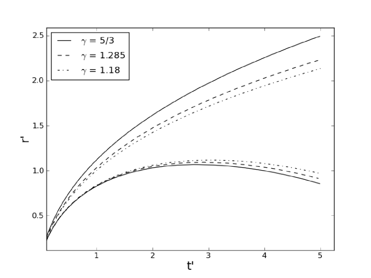
Figure 12: Evolution of the forward and reverse shocks with time for several values of the adiabatic index, $\gamma$, of the shocked medium. Top curves correspond to the forward shock; bottom curves correspond to the reverse shock. $t^{\prime}$ and $r^{\prime}$ are normalized to values given in Dwarkadas & Chevalier (1998). Solid line here corresponds to the solid line in Figure 2a of their paper. Note that decreasing $\gamma$ has the effect of shrinking the post-shock volume. Effective $\gamma$ values of 5/3, 1.285, and 1.18 correspond to effective $r$ values of 2.65, 4.8, and 6.8, respectively.

There is roughly a factor of 2-3 between our lower and upper limits to the pre-shock density. To explore both of these limits, we use the Virginia Hydrodynamics (VH-1) time-dependent hydrodynamic numerical code in one dimension. VH-1 is a hydrodynamics code which solves the Eulerian equations of fluid mechanics using the Piecewise Parabolic Method, described in Colella & Woodward (1984). We assume spherical symmetry on a numerical grid with 512 zones. We modify $r$ for the forward shock by varying the adiabatic index, $\gamma$ (= $\frac{5}{3}$ for a normal shock), of the shocked ambient medium (Blondin & Ellison, 2001). Softening the equation of state effectively makes the shocked plasma more compressible, yielding $r$ $>$ 4. We use the exponential ejecta density profiles of Dwarkadas & Chevalier (1998) and assume an explosion energy of $10^{51}$ ergs with an ejected mass of 1.4 $M_{\odot}$. In Figure 12, we plot the evolution of the forward and reverse shocks with time for varying values of $\gamma$, corresponding to immediate postshock $r$ values of 4, 8, and 12, using identical scalings to that of Dwarkadas & Chevalier (1998) (compare with Figure 2a of their paper).

With the mean post-shock density fixed at 6.2 cm^-3 (the gas density required to fit the spectrum assuming compact grains), we examined $r$ values of 12 and 25, corresponding to $\gamma$ values of 1.18 and 1.085, mean $r$ in the post-shock region of 6.8 and 12.5, and pre-shock densities of 0.91 and 0.50, respectively.

The lower density case, with $r=25$, reaches a radius of 3.6 pc in 550 years with a shock velocity at that time of 2950 km s^-1. While this age is roughly consistent with the known age of this object from light echoes, the shock velocity is too high to be consistent with the measured width of oxygen lines. This shock speed would imply a width, $v_{FWHM}$, of 5660 km s^-1. The measured value was $\sim 3500$ km s^-1. The higher density case requires 630 years to reach the observed radius, with a current shock speed of 2450 km s^-1. The line width implied from this shock speed is 4490 km s^-1. While this is still higher than our observed line width, it is much closer to being within the quoted errors, and is clearly favored over the lower density case.

Errors in determining the post-shock density from IR fits are about 20%, but this has almost no effect on the inferred pre-shock density allowed by not overpredicting oxygen lines in RGS spectra. However, this number is sensitive to the soft X-ray absorbing column density used in the models. If the LMC absorption component, detailed in Section 6.2, is increased, a higher pre-shock density will be allowed before oxygen lines are overproduced. To be within the errors of the line widths measured for oxygen lines, the LMC $N_{H}$ value would only need to be modestly increased from 1.6 to 1.7 $\times 10^{21}$ cm^-2. Kosenko et al. (2010) report an $N_{H}$ of 2.6 $\times 10^{21}$ cm^-2, which would easily accommodate a higher density. Uncertainties in the exact distance to the remnant are also non-negligible here. We assume a distance to the LMC of 50 kpc, but recent measurements of the distance to the LMC range from 47.8 kpc (Grocholski et al., 2007) to 51.1 kpc (Koerwer, 2009). The lower of these two would increase the observed radius of the remnant from 3.6 to 3.77 pc, which would bring the observed line width within errors of the shock velocity from hydro modeling. The unknown position of 0519 within the depth of the LMC may also be important.

7.4 Dust-to-Gas Mass Ratio

Of particular note in all results presented in Tables 2 and 3 is that given the amount of gas that these remnants have swept up at this stage of their evolution, the amount of dust observed by Spitzer is lower than what is expected, even accounting for the effects of sputtering (although there are a few values in Table 2 that are acceptable; namely, those with a high $r$). The amount of dust sputtered is $\sim 10$% for compact grains in 0509, and 34% for compact grains in 0519. UV studies of grain absorption in the ISM (Weingartner & Draine, 2001) yield a dust-to-gas mass ratio in the LMC of 2.5 $\times 10^{-3}$. Recent wide-field far-IR observations of the LMC give a value of $\sim 3.5\times 10^{-3}$ for this ratio (Meixner et al., 2010). This shortfall is consistent with our previous studies of both LMC and galactic SNRs (Borkowski et al., 2006; Williams et al., 2006; Blair et al., 2007). Similar results have been found for SN 1987A (Bouchet et al., 2006) in the LMC, although the shocks there probe circumstellar material, and have not yet reached the ambient ISM (but see Dwek et al. 2008,2010), and for G292.0+1.8 (Lee et al., 2009) and Puppis A (Arendt et al., 2010) in the Galaxy.

Of all parameters in the model, dust mass is the least model-dependent. As a check of this, we examine the case of 0519. Assuming compact grains, we derive a total radiating dust mass of 1.5 $\times 10^{-3}M_{\odot}$ based on model fits to IRS data. We then made fits to the data using a greatly simplified model, that of a single grain at a single temperature, ignoring heating, sputtering, and grain-size distribution. This model yielded a total dust mass of about 1.3 $\times 10^{-3}M_{\odot}$. As a further check, we used an approximate analytic expression from Dwek (1987) for the mass of dust, dependent only on the temperature of the grain and the observed IR luminosity, obtaining a value of 1.7 $\times 10^{-3}M_{\odot}$. These three different approaches of decreasing complexity only differ by at most a factor of 30%. Taking our minimum value of swept-up gas mass (5.3 $M_{\odot}$), we derive dust-to-gas mass ratios of 2.4-3.2 $\times 10^{-4}$, an order of magnitude lower than the expected value. Dust-to-gas mass ratios in 0509 are closer to expected values, but are, in most cases in Table 2, still too low. It may be that SNRs that are in regions of low background sufficient to allow a high enough signal-to-noise ratio for a detailed study in the mid- and far-IR have such a low background because they are in atypical regions of the ISM, creating an observational bias. In addition, dust-to-gas mass ratio determinations from SNRs are spot measurements, and are not averaged over long lines of sight or large fields of view.

Porous dust grains require a higher density relative to compact grains to reproduce the same spectrum, because they are more efficient radiators of energy than compact grains. For this reason, the inferred dust mass from the porous grain models, seen in Table 2, is lower by a factor of $\sim 2-4$. However, for a given $r$, the inferred gas mass is higher for porous grains, so that the dust-to-gas mass ratios for porous models are lower by a factor of $\sim 4$ for $\cal P$ = 25% and $\sim 18$ for $\cal P$ = 50%, when compared to the compact grain case. It should be noted though, that typical dust-to-gas mass ratios calculated for the ISM in general (such as the 0.25% given above from WD01) inherently assume compact grains.

One possibility that has been suggested for SNRs of both Type Ia and CC origin (Gomez et al., 2009; Dunne et al., 2003) is that large amounts of dust are indeed present, but are too cold (T_d $\sim 16$ K) to be detectable at Spitzer wavelengths and are only visible in the sub-millimeter regime. If this is true, then the total dust-to-gas mass ratio for the ISM could be quite different from what we report here, which is based only on “warm” dust. This claim has been disputed for Kepler’s SNR (Blair et al., 2007) based on a detection at 70 $\mu$m and an upper limit at 160 $\mu$m, but we lack detection at either wavelength here, and upper limits are unconstraining. Herschel observations would provide the key wavelength coverage between the mid-IR and sub-mm necessary to settle this issue. A recent Herschel observation of Cas A at wavelengths up to 500 $\mu$m revealed only 0.075 $M_{\odot}$ of dust there, much of which may be newly-formed ejecta dust (Barlow et al., 2010).

How cold would dust have to be to escape detection at 70 $\mu$m, assuming a standard dust-to-gas mass ratio for the LMC? Obviously, the answer depends on the choice of models from Tables 2 & 3. As an example, we consider the $\cal P$ = 0 model for 0519 with the highest value for $r$ (the only model for this remnant that seems to not be ruled out by X-ray lines). The swept gas mass for this case is 6.1 $M_{\odot}$, and assuming a dust-to-gas ratio of 0.35% gives a dust mass of 2.1 $\times 10^{-2}$ $M_{\odot}$. In order to avoid violating the 70 $\mu$m upper limit of 121 mJy (Borkowski et al., 2006), post-shock dust in this remnant would need to be $\mathrel{\mathchoice{\lower 3.1pt\vbox{\halign{$\m@th\displaystyle\hfil#\hfil$\cr<\crcr\sim\crcr}}}{\lower 3.1pt\vbox{\halign{$\m@th\textstyle\hfil#\hfil$\cr<\crcr\sim\crcr}}}{\lower 3.1pt\vbox{\halign{$\m@th\scriptstyle\hfil#\hfil$\cr<\crcr\sim\crcr}}}{\lower 3.1pt\vbox{\halign{$\m@th\scriptscriptstyle\hfil#\hfil$\cr<\crcr\sim\crcr}}}}44$ K. If we choose the standard $r$ case, the implied dust mass would be 5.5 $\times 10^{-2}$ $M_{\odot}$, and the required post-shock dust temperature would be $\mathrel{\mathchoice{\lower 3.1pt\vbox{\halign{$\m@th\displaystyle\hfil#\hfil$\cr<\crcr\sim\crcr}}}{\lower 3.1pt\vbox{\halign{$\m@th\textstyle\hfil#\hfil$\cr<\crcr\sim\crcr}}}{\lower 3.1pt\vbox{\halign{$\m@th\scriptstyle\hfil#\hfil$\cr<\crcr\sim\crcr}}}{\lower 3.1pt\vbox{\halign{$\m@th\scriptscriptstyle\hfil#\hfil$\cr<\crcr\sim\crcr}}}}36$ K. Both of these numbers are significantly lower than those fit to IRS data or those predicted by grain heating models. Such low temperatures could only be acheived by having the dust reside in very dense clumps. Shocks driven into such clumps should quickly become radiative, but no [O III] or [S II] emission is seen from either remnant.

8 Conclusions

We present mid-IR spectral observations of two young SNRs in the LMC, 0509-67.5 and 0519-69.0, as well as analysis of archival high-resolution X-ray spectra. By fitting dust heating and sputtering models to IR spectra, we can determine post-shock gas density. We derive post-shock densities of 0.59 and 6.2 cm^-3 in 0509 and 0519, respectively, using a compact grain model. Porous grains require a density higher by a factor of a few. By assuming a value for the shock compression ratio, $r$, we can infer the pre-shock density, swept gas mass, strength of oxygen Ly$\alpha$ and K$\alpha$ X-ray lines, and dust-to-gas mass ratio for the ambient ISM. Derived values for the pre-shock density of the ISM vary greatly depending on the model used and compression ratio assumed, but for the sake of comparison, values listed in Tables 2 & 3 are comparable to densities inferred from various line-of-sight HI column densities through the LMC. These column densities vary from 10²⁰ cm^-2 to a few $\times 10^{21}$ cm^-2, which, assuming an LMC depth of 1 kpc, yields densities of $\sim 0.05-1.5$. For standard strong shocks, $r$ is 4, but modification by cosmic rays would increase this by an unknown amount. We report values of the quantities above for several plausible values of $r$. In principle, this method could be used in reverse to determine $r$. This would require X-ray emission from shocked ambient medium that is well-separated from ejecta emission; thus, X-ray lines could be modeled as solely arising from material at cosmic abundances. We believe this method can be used for older, larger remnants in the LMC, such as DEM L71.

Based on our analysis, a significant fraction of the O line emission seen in the X-ray spectrum of 0509 arises from the ejecta. If grains are highly porous, then the ejecta contribution is less, but a contribution is still required because the line flux ratios observed still do not match the model ratios. Both standard shocks and cosmic-ray modified shocks with higher $r$ values can provide acceptable fits for 0509. The data for 0509 are inconclusive in favoring either compact or porous grains. Compact grains require nearly all of the oxygen seen in X-ray spectra to be coming from shocked ejecta, while porous grains would significantly lower the ejecta contribution, implying a higher contribution from the forward-shocked material.

In 0519, there is significant evidence for higher than standard compression, and little contribution from ejecta to O X-ray lines. A shock speed of $<$ 2300 km s^-1 is favored for this object from hydrodynamical simulations, in order to reproduce the observed size, age, and X-ray line widths. Compact grains are favored for this remnant. The standard value of $r=4$ is possible only if absorption to the remnant is significantly higher than has been reported. The column density from the LMC would need to be at least $4\times 10^{21}$ cm^-2 to bring oxygen lines in the model down to below observed values. Ghavamian et al. (2007) derive an upper limit for 0519 of $E(B-V)\leq 0.11$, implying an upper limit to the HI column density of $\sim 1.6$ $\times 10^{21}$ cm^-2 (Cox et al., 2006).

We derive dust-to-gas mass ratios that are lower by a factor of several than what is generally expected in the ISM. Since the general properties of dust in the ISM come from optical/UV absorption line studies averaged over long lines of sight, it is possible that there exist large local variations on smaller scales. The ratios presented here probe parsec scales. Another potential explanation is that the sputtering rate for dust grains is significantly understated in the literature. However, since the deficit of dust is about an order of magnitude, sputtering rates would also have to be increased by this amount to account for the discrepancy. Also, because sputtering rates typically assume a compact grain, further work in this field will be needed to determine if these rates are appropriate for porous grains. Extremely high values for $r$ ($>$ 50) could bring dust-to-gas mass ratios up to more typical values, but such values are ruled out by radio observations. A possible observational bias could exist, in that SNRs that are easy to study in the IR (i.e., well separated from sources of IR confusion) could be found preferentially in low-dust regions of the ISM.

Studies such as this will benefit greatly from the increases in both spatial resolution and sensitivity of future generations of telescopes, such as the James Webb Space Telescope. Being able to spatially separate the dust spectra right behind the shock from that further inside the shell will be crucial to reducing some of the uncertainties listed above. Longer wavelength observations with the Herschel Space Observatory would be useful for detecting or placing upper limits on any cold dust that may be present in the remnant.

Table 1: Model Input Parameters

Object	$V_{s}$ (km s-1)	$T_{e}$ (keV)	$T_{p}$ (keV)	Age (yrs.)	Ref.
B0509-67.5	6000	2.0	70	400	1, 2
B0519-69.0	3000	1.5	21	600	1, 2

Note. — References: (1) Ghavamian et al 2007, (2) Rest et al. 2005

Table 2: Predicted ISM Oxygen Line Strengths for SNR B0509-67.5

$\cal P$	$n_{H}$	$n_{0}$	$n_{e}t$	EM	O Ly$\alpha$	O K$\alpha$	MG	MD	MD/MG
0	0.59${}^{0.73}_{0.46}$	0.22${}^{0.28}_{0.17}$	2.97${}^{3.67}_{2.31}$ $\times 10^{9}$	0.089${}^{0.14}_{0.053}$	0.026${}^{0.044}_{0.015}$	0.1${}^{0.17}_{0.05}$	1.47${}^{1.82}_{1.15}$	1.90${}^{2.64}_{1.46}$ $\times 10^{-3}$	1.3${}^{2.3}_{0.8}$ $\times 10^{-3}$
0	0.59${}^{0.73}_{0.46}$	0.12${}^{0.15}_{0.1}$	2.97${}^{3.67}_{2.31}$ $\times 10^{9}$	0.048${}^{0.075}_{0.031}$	0.017${}^{0.026}_{0.012}$	0.054${}^{0.089}_{0.032}$	0.8${}^{0.99}_{0.62}$	1.90${}^{2.64}_{1.46}$ $\times 10^{-3}$	2.4${}^{4.3}_{1.5}$ $\times 10^{-3}$
0	0.59${}^{0.73}_{0.46}$	0.09${}^{0.11}_{0.068}$	2.97${}^{3.67}_{2.31}$ $\times 10^{9}$	0.036${}^{0.055}_{0.021}$	0.014${}^{0.021}_{0.01}$	0.041${}^{0.066}_{0.022}$	0.6${}^{0.74}_{0.47}$	1.90${}^{2.64}_{1.46}$ $\times 10^{-3}$	3.2${}^{5.6}_{1.9}$ $\times 10^{-3}$
25%	1.1${}^{1.4}_{0.9}$	0.42${}^{0.53}_{0.34}$	5.53${}^{7.0}_{4.52}$ $\times 10^{9}$	0.32${}^{0.51}_{0.21}$	0.12${}^{0.21}_{0.07}$	0.39${}^{0.61}_{0.26}$	2.80${}^{3.56}_{2.29}$	9.37${}^{12.2}_{6.81}$ $\times 10^{-4}$	3.3${}^{5.3}_{1.9}$ $\times 10^{-4}$
50%	2.2${}^{2.7}_{1.8}$	0.83${}^{1.02}_{0.68}$	1.11${}^{1.36}_{0.91}$ $\times 10^{10}$	1.25${}^{1.88}_{0.84}$	0.62${}^{0.98}_{0.39}$	1.30${}^{1.78}_{0.94}$	5.53${}^{6.78}_{4.52}$	4.1${}^{5.47}_{3.21}$ $\times 10^{-4}$	7.4${}^{12}_{4.7}$ $\times 10^{-5}$

Note. — Errors listed are 90% confidence intervals from $\chi^{2}$ fitting to the post-shock density in column 2. Porosity, $\cal P$, is percentage of grain occupied by vacuum. Three rows for compact grain case correspond to different values of shock compression ratio of 2.65, 4.8, and 6.8, as described in text. LMC abundances are assumed, so that $n_{e}$ = 1.2$n_{H}$. Line strengths are for shocked ISM, and are reported as fractions of observed line strengths measured from RGS spectra by model with absorption described in text. For this remnant, observed line strengths are: O Ly$\alpha$ = 4.41 $\times 10^{-13}$ ergs cm^-2 s^-1; O K$\alpha$ = 5.05 $\times 10^{-13}$ ergs cm^-2 s^-1. Models predicting fractional line fluxes of greater than 1 are ruled out. M_D is total amount of radiating dust, extrapolated from single slit position to entire remnant. M_D/M_G is ambient, pre-shock dust/gas ratio, where sputtering effects are accounted for.

Table 3: Predicted ISM Oxygen Line Strengths for SNR B0519-69.0

$\cal P$	$n_{H}$	$n_{0}$	$n_{e}t$	EM	O Ly$\alpha$	O K$\alpha$	MG	MD	MD/MG
0	6.2${}^{6.8}_{5.6}$	2.34${}^{2.57}_{2.11}$	4.69${}^{5.14}_{4.24}$ $\times 10^{10}$	9.92${}^{11.9}_{8.08}$	2.10${}^{2.41}_{1.77}$	2.63${}^{2.91}_{2.35}$	15.6${}^{17.1}_{14.1}$	1.95${}^{2.14}_{1.82}$ $\times 10^{-3}$	1.3${}^{1.5}_{1.1}$ $\times 10^{-4}$
0	6.2${}^{6.8}_{5.6}$	1.29${}^{1.42}_{1.17}$	4.69${}^{5.14}_{4.24}$ $\times 10^{10}$	5.47${}^{6.60}_{4.48}$	1.16${}^{1.34}_{0.99}$	1.46${}^{1.62}_{1.30}$	8.60${}^{9.43}_{7.77}$	1.95${}^{2.14}_{1.82}$ $\times 10^{-3}$	2.3${}^{2.8}_{1.9}$ $\times 10^{-4}$
0	6.2${}^{6.8}_{5.6}$	0.91${}^{1.0}_{0.82}$	4.69${}^{5.14}_{4.24}$ $\times 10^{10}$	3.86${}^{4.65}_{3.14}$	0.82${}^{0.95}_{0.70}$	1.02${}^{1.14}_{0.91}$	6.06${}^{6.65}_{5.47}$	1.95${}^{2.14}_{1.82}$ $\times 10^{-3}$	3.2${}^{3.9}_{2.7}$ $\times 10^{-4}$
25%	9.5${}^{10.3}_{8.6}$	3.58${}^{3.89}_{3.25}$	7.18${}^{7.79}_{6.50}$ $\times 10^{10}$	23.2${}^{27.4}_{1.91}$	3.83${}^{4.29}_{3.38}$	4.19${}^{4.60}_{3.79}$	23.9${}^{25.9}_{21.6}$	9.34${}^{10.2}_{8.74}$ $\times 10^{-4}$	3.9${}^{4.7}_{3.4}$ $\times 10^{-5}$
50%	17${}^{18.5}_{15.6}$	6.42${}^{6.98}_{5.89}$	1.29${}^{1.40}_{1.18}$ $\times 10^{11}$	74.6${}^{88.3}_{62.8}$	7.80${}^{8.45}_{7.05}$	7.95${}^{8.59}_{7.24}$	42.8${}^{46.6}_{39.3}$	4.80${}^{5.2}_{4.5}$ $\times 10^{-4}$	1.1${}^{1.3}_{0.97}$ $\times 10^{-5}$

Note. — Same as Table 2, except that measured line strengths from RGS data are as follows: O Ly$\alpha$ = 5.81 $\times 10^{-13}$ ergs cm^-2 s^-1; O K$\alpha$ = 3.91 $\times 10^{-13}$ ergs cm^-2 s^-1. Models predicting fractional line fluxes of greater than 1 are ruled out.

Figure 1: Top left: MIPS 24 $\mu$m image of SNR B0509-67.5, overlaid with regions of spectral extraction as described in text, where green region is “faint” region and yellow marks “bright” region. Top right: Star-subtracted H$\alpha$ image of 0509. Bottom left: MIPS 24 $\mu$m image of SNR B0519-69.0, with extraction slit shown in yellow. Bottom right: Star-subtracted H$\alpha$ image of 0519. Spectral extraction regions in both remnants are approximately 10.5^′′ $\times$ 45^′′. FWHM of MIPS 24 $\mu$m PSF is approximately 7^′′. H$\alpha$ images obtained with the 4-m Blanco telescope at NOAO/CTIO. In all images, north is up and east is to the left.

Figure 6: Left: H$\alpha$ image of B0509-67.5 from Figure 1, convolved with the MIPS 24 $\mu$m PSF. Right: MIPS 24 $\mu$m image, at native resolution.

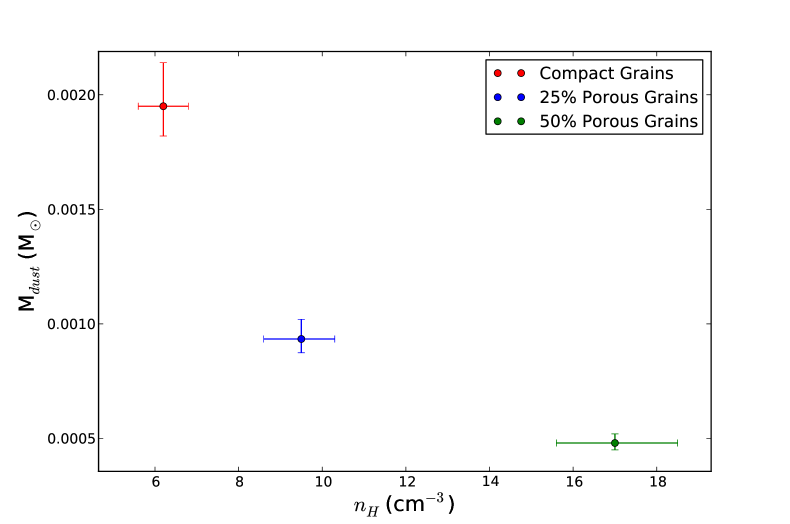
Figure 11: Same as Figure 10, but for 0519

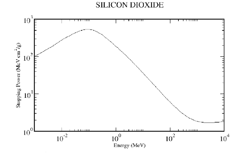
Figure 13: Stopping power of a proton in silicon dioxide (SiO₂) as a function of proton energy. Taken from the NIST PSTAR database (see text).

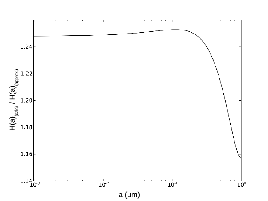
Figure 14: Ratio of proton heating rate of a silicate grain from calculations in this work to approximations from Draine & Salpeter (1979) & Dwek & Werner (1981) for an impinging particle energy of 100 keV, as a function of grain radius.

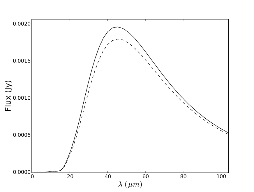
Figure 15: Comparison of spectra produced in dust heating model for protons of 100 keV. Solid line: spectrum assuming proton projected ranges calculated in Section 7.5. Dashed line: spectrum assuming analytical approximation to proton projected range from Draine & Salpeter (1979). Electron heating ($T_{e}$ = 2 keV) is included in this model. Projected range is defined as the average length traveled by a particle into a material.

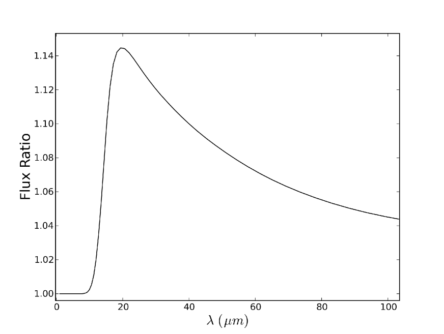
Figure 16: Ratio of spectra from Figure 15.

Appendix A Proton Energy Deposition Rates

In young SNRs, and in 0509 in particular, proton temperatures are much higher than electron temperatures, and heating by protons cannot be neglected as it can in slower shocks where temperatures have had time to equilibrate. Here we investigate whether simple analytic approximations to proton and alpha particle energy deposition rates are valid at ion energies approaching or exceeding 100 keV.

The stopping power (energy loss per unit path length) and projected range (average length traveled by a particle into a material) for both electrons and protons into a given grain are generally given by analytic expressions approximating experimental data. For electrons, these expressions fit the experimental data to within 15% for the energy range of 20 eV to 1 MeV (Dwek, 1987). For protons and alpha particles, the approximate stopping power, based on experimental data from Andersen & Ziegler (1977) and Ziegler (1977), is given by Draine & Salpeter (1979) as

$$R_{H}=3\times 10^{-6}\rho^{-1}(E/keV)g\ cm^{-2},R_{He}=0.6R_{H},$$ (A1)

where $\rho$ is the mass density of the grain. The authors caution that this expression is valid only for $E<100$ keV. We raise here two questions: 1) Are these approximations appropriate for energies at or exceeding the 100 keV threshold (as may well be the case in very young SNRs with shock speeds exceeding 6000 km s^-1)? 2) These approximations are based on data over 30 years old; are they still valid?

To answer both of these questions, we turn to more recent laboratory data on the stopping power of protons and alpha particles in various materials, obtained from the online PSTAR and ASTAR databases published and maintained by the National Institute of Standards and Technology. In Figure 13, we show the stopping power of a proton in silicon dioxide as a function of energy. The stopping power turns over above $\sim 100$ keV. Since, for an extremely fast shock, there will be a significant population of protons with energies in this range, this turnover should be properly accounted for in calculating the projected range of the particle.

Interstellar grains are more complicated than silicon dioxide (although it is possible that SiO₂ is a minor component of ISM dust). Since the NIST databases only have information available for actual materials that can be measured in the lab, materials like “astronomical silicate (MgFeSiO₄)” are not available. The individual stopping powers for the constituent elements are available, however, and can be combined to approximate the stopping power for a grain of arbitrary composition. To do this, we use “Bragg’s Rule,” (Bragg, 1905), given by

$$S(A_{m}B_{n})=m\cdot S(A)+n\cdot S(B),$$ (A2)

where $S(A_{m}B_{n})$ is the total stopping power of a molecule $A_{m}B_{n}$, and $S(A)$ and $S(B)$ are the stopping powers of the individual constituents. Since Mg is not included in the NIST database, we use the results of Fischer et al. (1996). Thus, for MgFeSiO₄, one has

$$S(MgFeSiO_{4})=S(Mg)+S(Fe)+S(Si)+4\cdot S(O).$$ (A3)

The calculated projected range for protons based on this stopping power (similarly for graphite) are given by the following polynomial expressions in logarithmic-space, where $E$ is the energy of the impinging particle in keV:

Protons

$$\log\ (R_{H,silicate})=0.053\ \log^{3}\ (E)-0.202\ \log^{2}\ (E)+1.21\ \log\ (E)-5.68$$ (A4)

$$\log\ (R_{H,graphite})=0.053\ \log^{3}\ (E)-0.158\ \log^{2}\ (E)+0.961\ \log\ (E)-5.46$$ (A5)

Alpha Particles

$$\log\ (R_{He,silicate}) = 3.78\times 10^{-3}\ \log^{5}\ (E)-8.79\times 10^{-3}\ \log^{4}\ (E)-4.25\times 10^{-2}\$$

$$\log^{3}\ (E)+6.25\times 10^{-2}\ \log^{2}\ (E)+1.04\ \log\ (E)-5.79$$

$$\log\ (R_{He,graphite}) = 3.33\times 10^{-3}\ \log^{5}\ (E)-6.13\times 10^{-3}\ \log^{4}\ (E)-3.46\times 10^{-2}\$$

$$\log^{3}\ (E)+3.03\times 10^{-2}\ \log^{2}\ (E)+0.966\ \log\ (E)-5.76.$$

Ultimately, it is necessary to determine how much energy is deposited into the grain by an impinging particle, in order to calculate grain heating rates and determine whether these improved energy deposition rates matter. In Figure 14, we show the ratio of the heating rate, $H(a,T)$, calculated from the NIST energy deposition rates and that calculated from the analytical approximations of Draine & Salpeter (1979) and Dwek & Werner (1981), for a proton temperature of 100 keV, which is relevant for the fast shocks, such as those seen in 0509. Figure 15 shows a comparison of the spectra of grains heated behind such a shock, for both the modified energy deposition rates described above and the analytical approximations. Figure 16 shows the ratio of the spectra. The main difference is in the 18-40 $\mu$m range, but the maximum difference is only $\sim 15$%. The use of analytical approximations to proton heating rates should be valid for most cases. Nonetheless, we use the modified rates in reporting results in this work.

A.1 Moving Grains

Because heating by protons is non-negligible in the case of such fast shocks and high ion temperatures, it is necessary to account for relative gas-grain motions between dust grains and ions in the plasma. Grain heating rates for protons and alpha particles are increased by 35 and 112%, respectively, over the case where grains are at rest with respect to the plasma. Grain heating is still dominated by electrons, though, so the overall heating rate is increased by only $\sim$ 25% for the moving grain case. When folded through the model, this results in a decrease of about 10% in the plasma densities necessary to fit IRS data. These numbers are reported throughout the text. We assume that the charge-to-mass ratio of the grains is sufficiently low that grains are not immediately affected by the passage of the shock.

References

- Andersen & Ziegler (1977) Andersen, H.H., & Ziegler, J.F. 1977, Hydrogen: Stopping Powers and Ranges in All Elements (New York: Pergamon)
- Arendt et al. (2010) Arendt. R.G., Dwek, E., Blair, W.P., Ghavamian, P., Hwang, U., Long, K.S., Petre, R., Rho, J., & Winkler, P.F. 2010, ApJ, 725, 585
- Badenes et al. (2008) Badenes, C., Hughes, J.P., Cassam-Chenai, G., & Bravo, E. 2008, ApJ, 680, 1149
- Badenes et al. (2003) Badenes, C., Bravo, E., Borkowski, K.J., & Dominguez, I. 2003, ApJ, 593, 358
- Barlow et al. (2010) Barlow, M.J., et al. 2010, A&A, 518, 138
- Berezhko & Ellison (1999) Berezhko, E.G. & Ellison, D.C. 1999, ApJ, 526, 385
- Blair et al. (2007) Blair, W.P., Ghavamian, P., Long, K.S., Williams, B.J., Borkowski, K.J., Reynolds, S.P., & Sankrit, R. 2007, ApJ, 662, 998
- Blondin & Ellison (2001) Blondin, J.M., & Ellison, D.C. 2001, ApJ, 560, 244
- Borkowski et al. (2001) Borkowski, K.J., Lyerly, W.J., & Reynolds, S.P. 2001, ApJ, 548, 820
- Borkowski et al. (2006) Borkowski, K.J., et al. 2006, ApJ, 642, 141, Paper I
- Bouchet et al. (2006) Bouchet, P., et al. 2006, ApJ, 650, 212
- Bragg (1905) Bragg, W.H., & Kleeman, L. 1905, Phil. Mag. 10, 318
- Clayton et al. (2003) Clayton, G.C., Wolff, M.J., Sofia, U.J., Gordon, K.D., & Misselt, K.A. 2003, ApJ, 588, 871
- Cox et al. (2006) Cox, N.L.J., Cordiner, M.A., Cami, J., Foing, B.H., Sarre, P.J., Kaper, L., & Ehrenfreund, P. 2006, A&A, 447, 991
- Colella & Woodward (1984) Colella, P., & Woodward, P.R. 1984, J. of Comp. Phys., 54, 174
- Dickel & Milne (1995) Dickel, J.R., & Milne, D.K. 1995, AJ, 109, 200
- Draine & Salpeter (1979) Draine, B. T., & Salpeter, E. E. 1979, ApJ, 231, 77
- Dunne et al. (2003) Dunne, L. et al. 2003, Nature, 424, 285
- Dwarkadas & Chevalier (1998) Dwarkadas, V. V., & Chevalier, R.A. 1993, ApJ, 497, 807
- Dwek (1987) Dwek, E., 1987, ApJ, 322, 812
- Dwek & Werner (1981) Dwek, E., & Werner, M.W. 1981, ApJ, 248, 138
- Dwek et al. (2008) Dwek, E. at al. 2008, ApJ, 676, 1029
- Fischer et al. (1996) Fischer, P., Eppacher, C., Hofler, G., & Semrad, D. 1996, Nucl. Instrum. Methods Phys. Res., 218, 817
- Ghavamian et al. (2007) Ghavamian, P., Blair, W.P., Sankrit, R., Raymond, J.C., & Hughes, J.P. 2007, ApJ, 664, 304
- Gomez et al. (2009) Gomez, H.L., Dunne, L., Ivison, R.J., Reynoso, E.M., Thompson, M.A., Sibthorpe, B., Eales, S.A., DeLaney, T.M., Maddox, S., Isaak, K. 2009, MNRAS, 397, 1621
- Grocholski et al. (2007) Grocholski, A.J., Sarajedini, A., Olsen, K.A.G., Tiede, G.P., & Mancone, C.L. 2007, AJ, 134, 680
- Helder et al. (2010) Helder, E.A., Kosenko, D., & Vink, J., 2010, arXiv:1007.3138
- Hughes et al. (1995) Hughes, J.P., et al. 1995, ApJ, 444, 81
- Hughes et al. (2007) Hughes, A., Staveley-Smith, L., Kim, S., Wolleben, M., Filipović, M. 2007, MNRAS.382, 543
- Jones & Ellison (1991) Jones, F.C. & Ellison, D.C. 1991, Spa. Sci. Rev., 58, 259
- Jurac et al. (1998) Jurac, S., Johnson, R.E., & Donn, B. 1998, ApJ, 503, 247
- Koerwer (2009) Koerwer, J.F. 2009, AJ, 138, 1
- Kosenko et al. (2008) Kosenko, D., Vink, J., Blinnikov, S., Rasmussen, A. 2008, A&A, 490, 223
- Kosenko et al. (2010) Kosenko, D., Helder, E., Vink, J. 2010, arXiv:1001.0983
- Lee et al. (2009) Lee, H. et al. 2009, ApJ, 706, 441
- Marion et al. (2009) Marion, G.H., Hoeflich, P., Gerardy, C.L., Vacca, W.D., Wheeler, J.C., Robinson, E.L. 2009, AJ, 138, 727
- Mathis (1996) Mathis, J.S., 1996, ApJ, 472, 643
- Meixner et al. (2010) Meixner, M., et al. 2010, A & A, 518, L71
- Mills et al. (1984) Mills, B.Y., Turtle, A.J., Little, A.G., & Durdin, J.M. 1984, Austr.J.Phys., 37, 321.
- Nozawa et al. (2006) Nozawa, T., Kozasa, T., & Habe, A. 2006, ApJ, 648, 435
- Pacholczyk (1970) Pacholczyk, A.G. 1970, Radio Astrophysics (San Francisco: Freeman).
- Rest et al. (2005) Rest, A., et al. 2005, Nature, 438, 1132
- Seok et al. (2008) Seok, J., et al. 2008, PASJ, 60, 453
- Serra Dìaz-Cano & Jones (2008) Serra Dìaz-Cano, L. & Jones, A.P. 2008, A&A, 492, 127
- Shen et al. (2008) Shen, Y., Draine, B.T., & Johnson, E.T. 2008, ApJ, 689, 260
- Smith et al. (1991) Smith, R.C., Kirshner, R.P., Blair, W.P., & Winkler, P.F. 1991, ApJ, 375, 652
- Staveley-Smith et al. (2003) Staveley-Smith, L., Kim, S., Calabretta, M.R., Haynes, R.F., & Kesteven, M.J. 2003, MNRAS, 339, 87
- Tuohy et al. (1982) Tuohy, I. R., Dopita, M. A., Mathewson, D. S., Long, K.S., & Helfand, D. J. 1982, ApJ, 261, 473
- Vink et al. (2010) Vink, J., Yamakazi, R., Helder, E.A., & Schure, K.M. 2010, ApJ, 722, 1727
- Warren & Hughes (2004) Warren, J.S., & Hughes, J.P. 2004, ApJ, 608, 261
- Weingartner & Draine (2001) Weingartner, J.C., & Draine, B.T. 2001, ApJ, 548, 296
- Williams et al. (2006) Williams, B.J., et al. 2006, ApJ, 652, 33
- Williams (2010) Williams, B.J. 2010, Ph.D. Thesis, arXiv:1005:1296
- Wilms et al. (2000) Wilms, J., Allen, A. & McCray, R. 2000, ApJ, 542, 914
- Ziegler (1977) Ziegler, J.F. 1977, Helium: Stopping Powers and Ranges in All Elements (New York: Pergamon)