On the linear algebra of local complementation

Abstract

We explore the connections between the linear algebra of symmetric matrices over $GF(2)$ and the circuit theory of 4-regular graphs. In particular, we show that the equivalence relation on simple graphs generated by local complementation can also be generated by an operation defined using inverse matrices.

Keywords. Euler circuit, interlacement, inverse matrix, local complement, pivot

Mathematics Subject Classification. 05C50

1 Introduction

This paper is about the connection between the circuit theory of 4-regular multigraphs and the elementary linear algebra of symmetric matrices over the two-element field $GF(2)$.

Definition 1

A square matrix $S=(s_{ij})$ with entries in $GF(2)$ is symmetric if $s_{ij}=s_{ji}$ for all $i\neq j$. $S$ is zero-diagonal if $s_{ii}=0$ for all $i$.

As $GF(2)$ is the only field that concerns us, we will often omit the phrase “with entries in $GF(2)$.”

Symmetric matrices are important to us because they arise as adjacency matrices of graphs, and for our purposes it is not important if the vertices of a graph are listed in any particular order. That is, if $V$ is a finite set then we regard a $V\times V$ matrix as a function $V^{2}\rightarrow GF(2)$. Of course we must impose an order on $V$ in order to display a matrix.

Many zero-diagonal symmetric matrices are singular, and consequently do not have inverses in the usual sense. Nevertheless matrix inversion gives rise to an interesting relation among zero-diagonal symmetric matrices.

Definition 2

Let $S$ be a zero-diagonal symmetric matrix. A modified inverse of $S$ is a zero-diagonal symmetric matrix obtained as follows: first toggle some diagonal entries of $S$ to obtain an invertible symmetric matrix $S^{\prime}$, and then toggle every nonzero diagonal entry of $(S^{\prime})^{-1}$.

Here toggling refers to the function $x\mapsto x+1$, which interchanges the elements of $GF(2)$.

The relation defined by modified inversion is obviously symmetric, but examples indicate that it is not reflexive or transitive.

Example 3

For each of these four matrices, the set of modified inverses consists of the other three.

$$\begin{pmatrix}0&1&1\\ 1&0&1\\ 1&1&0\end{pmatrix}\text{ \ }\begin{pmatrix}0&1&1\\ 1&0&0\\ 1&0&0\end{pmatrix}\text{ }\begin{pmatrix}0&1&0\\ 1&0&1\\ 0&1&0\end{pmatrix}\text{ }\begin{pmatrix}0&0&1\\ 0&0&1\\ 1&1&0\end{pmatrix}$$

Example 4

The modified inverses of the first of the following three matrices include the other two, but not itself. The modified inverses of the second include the first, but not itself or the third. The modified inverses of the third include the first and itself, but not the second.

$$\text{\ }\begin{pmatrix}0&0&1&0\\ 0&0&0&1\\ 1&0&0&1\\ 0&1&1&0\end{pmatrix}\text{ \ }\begin{pmatrix}0&1&1&0\\ 1&0&1&1\\ 1&1&0&0\\ 0&1&0&0\end{pmatrix}\text{ \ }\begin{pmatrix}0&1&1&1\\ 1&0&1&0\\ 1&1&0&1\\ 1&0&1&0\end{pmatrix}$$

Definition 2 yields an equivalence relation in the usual way.

Definition 5

Let $S$ and $T$ be zero-diagonal symmetric $GF(2)$-matrices. Then $S\sim_{mi}T$ if $T$ can be obtained from $S$ through a finite (possibly empty) sequence of modified inversions.

We recall some relevant definitions from graph theory. In a 4-regular multigraph every vertex is of degree 4. Loops and parallel edges are allowed; a loop contributes twice to the degree of the incident vertex. In order to distinguish between the two orientations of a loop it is technically necessary to consider half-edges rather than edges; we will often leave it to the reader to refine statements regarding edges accordingly. A walk in a 4-regular graph is a sequence $v_{1},h_{1},h_{2}^{\prime},v_{2},h_{2},h_{3}^{\prime},...,h_{k-1},h_{k}^{\prime},v_{k}$ such that for each $i$, $h_{i}$ and $h_{i}^{\prime}$ are distinct half-edges incident on $v_{i}$, and $h_{i}$ and $h_{i+1}^{\prime}$ are half-edges of a single edge. The walk is closed if $v_{1}=v_{k}$. A walk in which no edge is repeated is a trail, and a closed trail is a circuit. An Euler circuit is a circuit that contains every edge of the graph. Every connected 4-regular multigraph has Euler circuits, and every 4-regular multigraph has Euler systems, each of which contains one Euler circuit for every connected component of the graph.

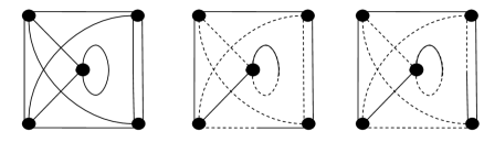
Figure 1: A 4-regular multigraph with two of its Euler circuits. To trace an Euler circuit, maintain the dash pattern while traversing each vertex. (The dash pattern may change within an edge, though.)

For example, Figure 1 illustrates two Euler circuits in a connected 4-regular multigraph. These two Euler circuits illustrate the following.

Definition 6

If $C$ is an Euler system of a 4-regular multigraph $F$ and $v\in V(F)$ then the $\kappa$-transform $C\ast v$ is the Euler system obtained by reversing one of the two $v$-to-$v$ trails within the circuit of $C$ incident at $v$.

The $\kappa$-transformations were introduced by Kotzig [34], who proved the fundamental fact of the circuit theory of 4-regular multigraphs.

Theorem 7

(Kotzig’s theorem) All the Euler systems of a 4-regular multigraph can be obtained from any one by applying finite sequences of $\kappa$-transformations.

In this paper our attention is focused on 4-regular multigraphs, but we should certainly mention that the reader interested in general Eulerian multigraphs will find Fleischner’s books [21, 22] uniquely valuable. In particular, Theorem VII.5 of [21] generalizes Kotzig’s theorem to arbitrary Eulerian graphs.

The alternance or interlacement graph $\mathcal{I}(C)$ associated to an Euler system $C$ of a 4-regular multigraph $F$ was introduced shortly after Kotzig’s work became known [7, 19, 42]. Two vertices $v\neq w$ of $F$ are interlaced with respect to $C$ if and only if they appear in the order $v...w...v...w$ on one of the circuits included in $C$.

Definition 8

The interlacement graph of a 4-regular graph $F$ with respect to an Euler system $C$ is the simple graph $\mathcal{I}(F,C)$ with $V(\mathcal{I}(F,C))=V(F)$ and $E(\mathcal{I}(F,C))=\{vw$ $|$ $v$ and $w$ are interlaced with respect to $C\}$. The interlacement matrix of $F$ with respect to $C$ is the adjacency matrix of this graph; when no confusion can arise, we use $\mathcal{I}(C)$ to denote both the graph and the matrix.

A simple graph that can be realized as an interlacement graph is called a circle graph, and Kotzig’s $\kappa$-transformations give rise to the fundamental operation of the theory of circle graphs, which we call simple local complementation. This operation has been studied by Bouchet [8, 9, 10], de Fraysseix [23], and Read and Rosenstiehl [42], among others. The reader can easily verify that the effect of a $\kappa$-transformation on an interlacement matrix is described as follows.

Definition 9

Let $S$ be a symmetric $n\times n$ matrix, and suppose $1\leq i\leq n$. Then the simple local complement of $S$ at $i$ is the symmetric $GF(2)$-matrix $S^{i}$ obtained from $S$ as follows: whenever $i\neq j\neq k\neq i$ and $s_{ij}\neq 0\neq s_{ik}$, toggle $s_{jk}$.

We call this operation simple local complementation to distinguish it from the similar operation that Arratia, Bollobás and Sorkin called local complementation in [1, 2, 3]. The two operations differ on the diagonal:

Definition 10

Let $S$ be a symmetric $n\times n$ matrix, and suppose $1\leq i\leq n$. Then the (non-simple) local complement of $S$ at $i$ is the symmetric matrix $S_{ns}^{i}$ obtained from $S^{i}$ as follows: whenever $j\neq i$ and $s_{ij}\neq 0$, toggle $s_{jj}$.

The first $3\times 3$ matrix of Example 3 has three distinct simple local complements, which are the same as its three modified inverses. Each of the three other $3\times 3$ matrices of Example 3 has only two distinct simple local complements, itself and the first matrix.

Definition 11

Let $S$ and $T$ be zero-diagonal symmetric $GF(2)$-matrices. Then $S\sim_{lc}T$ if $T$ can be obtained from $S$ through a finite (possibly empty) sequence of simple local complementations.

Proposition 12

This defines an equivalence relation.

Proof. As $(S^{i})^{i}=S$, $\sim_{lc}$ is symmetric. The reflexive and transitive properties are obvious.   

In Section 3 we prove a surprising result:

Theorem 13

Let $S$ and $T$ be zero-diagonal symmetric $GF(2)$-matrices. Then $S\sim_{lc}T$ if and only if $S\sim_{mi}T$.

We might say that modified inversion constitutes a kind of global complementation of a zero-diagonal symmetric matrix (or equivalently, a simple graph). Theorem 13 shows that even though individual global complementations do not generally have the same effect as individual simple local complementations, the two operations generate the same equivalence relation.

Theorem 13 developed as we read the work of several authors who have written about the equivalence relation on looped graphs (or equivalently, symmetric $GF(2)$-matrices) generated by (non-simple) local complementations at looped vertices and pivots on unlooped edges; we denote this relation $\sim_{piv}$. (If $G$ is a looped graph then a pivot on an unlooped edge $ab$ of $G$ is the triple simple local complement $((G^{a})^{b})^{a}=((G^{b})^{a})^{b}$.) Although $\sim_{piv}$ is defined for symmetric matrices and $\sim_{lc}$ is defined only for zero-diagonal symmetric matrices, it is reasonable to regard $\sim_{lc}$ as a coarser version of $\sim_{piv}$, obtained by ignoring the difference between looped and unlooped vertices. Genest [24, 25] called the equivalence classes under $\sim_{piv}$ Sabidussi orbits. Glantz and Pelillo [26] and Brijder and Hoogeboom [16, 17, 18] observed that another way to generate $\sim_{piv}$ is to use a matrix operation related to inversion, the principal pivot transform [48, 49]. In particular, Theorem 24 of [17] shows that the combination of loop-toggling with $\sim_{piv}$ yields a description of $\sim_{lc}$ that is different from Definition 9 (and also Definition 2). Ilyutko [28, 29] has also studied inverse matrices and the equivalence relation $\sim_{piv}$; he used them to compare the adjacency matrices of certain kinds of chord diagrams that arise from knot diagrams. Ilyutko’s account includes an analysis of the effect of the Reidemeister moves of knot theory, and also includes the idea of generating an equivalence relation on nonsingular symmetric matrices by toggling diagonal entries. Considering the themes shared by these results, it seemed natural to wonder whether the connection between matrix inversion and $\sim_{piv}$ reflects a connection between matrix inversion and the coarser equivalence relation $\sim_{lc}$.

Theorem 13 is part of a very pretty theory tying the elementary linear algebra of symmetric $GF(2)$-matrices to the circuit theory of 4-regular multigraphs. This theory has been explored by several authors over the last forty years, but the relevant literature is fragmented and it does not seem that the generality and simplicity of the theory are fully appreciated. We proceed to give an account.

At each vertex of a 4-regular multigraph there are three transitions – three distinct ways to sort the four incident half-edges into two disjoint pairs. Kotzig [34] introduced this notion, and observed that each of the $3^{n}$ ways to choose one transition at each vertex yields a partition of $E(F)$ into edge-disjoint circuits; such partitions are called circuit partitions [1, 2, 3] or Eulerian partitions [35, 38]. (Kotzig actually used the term transition in a slightly different way, to refer to only one pair of half-edges. As we have no reason to ever consider a single pair of half-edges without also considering the complementary pair, we follow the usage of Ellis-Monaghan and Sarmiento [20] and Jaeger [31] rather than Kotzig’s.)

In [47] we introduced the following way to label the three transitions at $v$ with respect to a given Euler system $C$. Choose either of the two orientations of the circuit of $C$ incident at $v$, and use $\phi$ to label the transition followed by this circuit; use $\chi$ to label the other transition in which in-directed edges are paired with out-directed edges; and use $\psi$ to label the transition in which the two in-directed edges are paired with each other, and the two out-directed edges are paired with each other. See Figure 2, where the pairings of half-edges are indicated by using solid line segments for one pair and dashed line segments for the other.

Figure 2: The three transitions at a vertex are labeled according to their relationships with the incident circuit of $C$.

Definition 14

Let $C$ be an Euler system of a 4-regular multigraph $F$, and let $P$ be a circuit partition of $F$. The relative interlacement matrix $\mathcal{I}_{P}(C)$ of $P$ with respect to $C$ is obtained from $\mathcal{I}(C)$ by modifying the row and column corresponding to each vertex at which $P$ does not involve the transition labeled $\chi$ with respect to $C$:

(i) If $P$ involves the $\phi$ transition at $v$, then modify the row and column of $\mathcal{I}(C)$ corresponding to $v$ by changing every nonzero entry to $0$, and changing the diagonal entry from 0 to 1.

(ii) If $P$ involves the $\psi$ transition at $v$, then modify the row and column of $\mathcal{I}(C)$ corresponding to $v$ by changing the diagonal entry from 0 to 1.

The relative interlacement matrix determines the number of circuits included in $P$:

$$\nu(\mathcal{I}_{P}(C))+c(F)=\left|P\right|,$$

where $\nu(\mathcal{I}_{P}(C))$ denotes the $GF(2)$-nullity of $\mathcal{I}_{P}(C)$ and $c(F)$ denotes the number of connected components in $F$. We refer to this equation as the circuit-nullity formula or the extended Cohn-Lempel equality; many special cases and reformulations have appeared over the years [5, 6, 8, 15, 19, 30, 32, 33, 36, 37, 39, 40, 43, 44, 45, 50]. A detailed account is given in [46].

The circuit-nullity formula is usually stated in an equivalent form, with part (i) of Definition 14 replaced by:

(i)^′ If $P$ involves the $\phi$ transition at $v$, then remove the row and column of $\mathcal{I}(C)$ corresponding to $v$.

We use (i) instead because it is more convenient for the sharper form of the circuit-nullity formula given in Theorem 16, which includes a precise description of the nullspace of $\mathcal{I}_{P}(C)$.

Definition 15

Let $P$ be a circuit partition of the 4-regular multigraph $F$, and let $C$ be an Euler system of $F$. For each circuit $\gamma\in P$, let the relative core vector of $\gamma$ with respect to $C$ be the vector $\rho(\gamma,C)\in GF(2)^{V(F)}$ whose nonzero entries correspond to the vertices of $F$ at which $P$ involves either the $\chi$ or the $\psi$ transition, and $\gamma$ is singly incident. (A circuit $\gamma$ is singly incident at $v$ if $\gamma$ includes precisely two of the four half-edges at $v$.)

Theorem 16

Let $P$ be a circuit partition of the 4-regular multigraph $F$, and let $C$ be an Euler system of $F$.

(i) The nullspace of the relative interlacement matrix $\mathcal{I}_{P}(C)$ is spanned by the relative core vectors of the circuits of $P$.

(ii) For each connected component of $F$, the relative core vectors of the incident circuits of $P$ sum to $0$.

(iii) If $Q\subset P$ and there is no connected component of $F$ for which $Q$ contains every incident circuit of $P$, then the relative core vectors of the circuits of $Q$ are linearly independent.

Theorem 16 is an example of a comment made above, that the generality and simplicity of the relationship between linear algebra and the circuit theory of 4-regular multigraphs have not been fully appreciated.

On the one hand, Theorem 16 is general: it applies to every 4-regular multigraph $F$, every Euler system $C$ and every circuit partition $P$. In Proposition 4 of [30], Jaeger proved an equivalent version of the special case of Theorem 16 involving the additional assumptions that $F$ is connected and $C$ and $P$ involve different transitions at every vertex. (These assumptions are implicit in Jaeger’s use of left-right walks on chord diagrams.) It is Jaeger who introduced the term core vector; we use relative core vector to reflect the fact that in Definition 15, the vector is adjusted according to the Euler system with respect to which it is defined. We provide a direct proof of Theorem 16 in Section 4 below, but the reader who is already familiar with Jaeger’s special case may deduce the general result using detachment [21, 41] along $\phi$ transitions. Bouchet [8] gave a different proof with the additional restriction that $C$ and $P$ respect a fixed choice of edge-direction in $F$; or equivalently, that $P$ involve only transitions that are labeled $\chi$ with respect to $C$. (Bouchet’s result is also presented in [27].) Genest [24, 25] did not use techniques of linear algebra, but he did discuss the use of bicolored graphs to represent a circuit partition $P$ using an Euler system that does not share a transition with $P$ at any vertex. These previous results may give the erroneous impression that an Euler system provides information about only those circuit partitions that disagree with it at every vertex. In fact, every Euler system gives rise to a mapping

$$\{\text{circuit partitions of }F\}\rightarrow\{\text{subspaces of }GF(2)^{V(F)}\}$$

under which the image of an arbitrary circuit partition $P$ is the $(\left|P\right|-c(F))$-dimensional subspace spanned by the relative core vectors of the circuits in $P$.

On the other hand, Theorem 16 is simple: Definition 14 gives an explicit description of the relative interlacement matrix associated to a circuit partition, and Definition 15 gives an explicit description of its nullspace. Although some version of Theorem 16 may be implicit in the theory of delta-matroids, isotropic systems and multimatroids associated with 4-regular graphs (cf. for instance [11, 12, 13, 14]), these structures are sufficiently abstract that it is difficult to extract explicit descriptions like Definition 14 and Definition 15 from them.

The circuit-nullity formula implies that if $C$ is an Euler system of $F$, then we can find every other Euler system $C^{\prime}$ of $F$ by finding every way to obtain a nonsingular matrix from $\mathcal{I}(C)$ using the modifications given in Definition 14. Moreover, there is a striking symmetry tying together the relative interlacement matrices of two Euler systems:

Theorem 17

Let $F$ be a 4-regular graph with Euler systems $C$ and $C^{\prime}$. Then

$$\mathcal{I}_{C^{\prime}}(C)^{-1}=\mathcal{I}_{C}(C^{\prime}).$$

Like Theorem 16, Theorem 17 generalizes results of Bouchet and Jaeger discussed in [8, 27, 30], which include the additional assumption that $C$ and $C^{\prime}$ are compatible (i.e., they do not involve the same transition at any vertex). Bouchet’s version requires also that $C$ and $C^{\prime}$ respect the same edge-directions.

Greater generality is always desirable, of course, but it is important to observe that in fact, Theorem 17 is particularly valuable when $C$ and $C^{\prime}$ are compatible. The equation $\mathcal{I}_{C^{\prime}}(C)^{-1}=\mathcal{I}_{C}(C^{\prime})$ does not allow us to construct the full interlacement matrix $\mathcal{I}(C^{\prime})$ directly from $\mathcal{I}(C)$ if $C$ and $C^{\prime}$ share a transition at any vertex, because there is no way to recover the information that is lost when off-diagonal entries are set to $0$ in part (i) of Definition 14. (For instance, if $C$ is any Euler system and $v$ is any vertex then Definition 14 tells us that $\mathcal{I}_{C}(C)=\mathcal{I}_{C}(C\ast v)=\mathcal{I}_{C\ast v}(C)$ is the identity matrix no matter how $C$ is structured.) This observation motivates our last definition.

Definition 18

Let $F$ be a 4-regular multigraph with an Euler system $C$, and suppose $W\subseteq V(F)$ has the property that an Euler system is obtained from $C$ by using the $\psi$ transition at every vertex in $W$, and the $\chi$ transition at every vertex not in $W$. Then this Euler system is the $\iota$-transform of $C$ with respect to $W$; we denote it $C\#W$.

According to the circuit-nullity formula, $C\#W$ is an Euler system if and only if a nonsingular matrix $M$ is obtained from $\mathcal{I}(C)$ by changing the diagonal entries corresponding to elements of $W$ from $0$ to $1$. Then $M=\mathcal{I}_{C\#W}(C)$ and $M^{-1}=\mathcal{I}_{C}(C\#W)$, so $\mathcal{I}(C)$ and $\mathcal{I}(C\#W)$ are modified inverses. We call the process of obtaining $C\#W$ from $C$ an $\iota$-transformation in recognition of this connection with matrix inversion.

Theorem 13 and the fact that simple local complementations correspond to $\kappa$-transformations imply the following alternative to Kotzig’s theorem:

Theorem 19

All the Euler systems of a 4-regular multigraph can be obtained from any one by applying finite sequences of $\iota$-transformations.

Figure 3: An Euler circuit of $C$ incident at a vertex $v$, along with the four different ways $C\#W$ might be configured at $v$.

The fact that the full interlacement matrix $\mathcal{I}(C\#W)$ is determined by $\mathcal{I}(C)$ and $W$ implies that the transition labels of $C\#W$ are also determined. Suppose $v\in V(F)$; we use $\phi,\chi,\psi$ to label the three transitions at $v$ with respect to $C$, and $\phi^{\prime},\chi^{\prime},\psi^{\prime}$ to label the three transitions at $v$ with respect to $C\#W$. Let $M$ denote the nonsingular matrix obtained from $\mathcal{I}(C)$ by toggling the diagonal entries corresponding to elements of $W$, and let $X\subseteq V(F)$ denote the set of vertices corresponding to nonzero diagonal entries of $M^{-1}$. Then $\phi^{\prime}=\psi$ if $v\in W$, $\phi^{\prime}=\chi$ if $v\not\in W$, $\phi=\psi^{\prime}$ if $v\in X$ and $\phi=\chi^{\prime}$ if $v\notin X$. Consequently $v\in W\cap X$ implies $\phi^{\prime}=\psi$, $\phi=\psi^{\prime}$ and $\chi=\chi^{\prime}$; $v\in W-X$ implies $\phi^{\prime}=\psi$, $\phi=\chi^{\prime}$ and $\chi=\psi^{\prime}$; $v\in X-W$ implies $\phi^{\prime}=\chi$, $\phi=\psi^{\prime}$ and $\psi=\chi^{\prime}$; and $v\in V(F)-W-X$ implies $\phi^{\prime}=\chi$, $\phi=\chi^{\prime}$ and $\psi=\psi^{\prime}$. See Figure 3, where the four cases are indexed by first listing $\phi^{\prime}$ with respect to $C$ and then listing $\phi$ with respect to $C^{\prime}$, so that $\chi\psi^{\prime}$ represents $v\in X-W$, $\psi\psi^{\prime}$ represents $v\in W\cap X$, $\psi\chi^{\prime}$ represents $v\in W-X$ and $\chi\chi^{\prime}$ represents $v\in V(F)-W-X$.

Theorem 17 also implies that interlacement matrices satisfy a limited kind of multiplicative functoriality, which we have not seen mentioned elsewhere.

Corollary 20

Let $C$ and $C^{\prime}$ be Euler systems of a 4-regular multigraph $F$, and let $P$ be the circuit partition described by: (a) at every vertex where $C$ and $C^{\prime}$ involve the same transition, $P$ involves the same transition; and (b) at every vertex where $C$ and $C^{\prime}$ involve two different transitions, $P$ involves the third transition. Then

$$\mathcal{I}_{P}(C)=\mathcal{I}_{C^{\prime}}(C)\cdot\mathcal{I}_{P}(C^{\prime}).$$

Proof. Let $I$ be the identity matrix, and let $I^{\prime}$ be the diagonal matrix whose $vv$ entry is $1$ if and only if $C$ and $C^{\prime}$ involve different transitions at $v$. Then

$$\mathcal{I}_{P}(C)=I^{\prime}+\mathcal{I}_{C^{\prime}}(C)=I+\mathcal{I}_{C^{\prime}}(C)\cdot I^{\prime}$$

$$=\mathcal{I}_{C^{\prime}}(C)\cdot(\mathcal{I}_{C}(C^{\prime})+I^{\prime})=\mathcal{I}_{C^{\prime}}(C)\cdot\mathcal{I}_{P}(C^{\prime}).$$

 

Corollary 21

Suppose a 4-regular multigraph $F$ has three pairwise compatible Euler systems $C$, $C^{\prime}$ and $C^{\prime\prime}$. (That is, no two of $C,C^{\prime},C^{\prime\prime}$ involve the same transition at any vertex). Then

$$\mathcal{I}_{C}(C^{\prime})\cdot\mathcal{I}_{C^{\prime\prime}}(C)\cdot\mathcal{I}_{C^{\prime}}(C^{\prime\prime})$$

is the identity matrix.

Proof. By Corollary 20, $\mathcal{I}_{C^{\prime\prime}}(C)=\mathcal{I}_{C^{\prime}}(C)\cdot\mathcal{I}_{C^{\prime\prime}}(C^{\prime})$.   

2 Examples

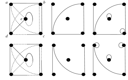
Figure 4: Two Euler circuits in the graph of Figure 1, the interlacement graphs $\mathcal{I}(C)$ and $\mathcal{I}(C^{\prime})$, and the looped graphs with adjacency matrices $\mathcal{I}_{C^{\prime}}(C)$ and $\mathcal{I}_{C}(C^{\prime})$.

Before giving proofs we discuss some illustrative examples. In the first column of Figure 4 we see two Euler circuits $C$ and $C^{\prime}$ in the graph $F$ of Figure 1. $C$ is given by the double occurrence word $abcdbcaeed$, and $C^{\prime}$ is given by $abcbdeeadc$. In the second column we see the simple graphs $\mathcal{I}(C)$ and $\mathcal{I}(C^{\prime})$, and in the third column we see the looped graphs whose adjacency matrices are

$$\text{ }\mathcal{I}_{C^{\prime}}(C)=\begin{pmatrix}0&0&0&1&0\\ 0&0&1&1&0\\ 0&1&1&1&0\\ 1&1&1&0&0\\ 0&0&0&0&1\end{pmatrix}\text{ and }\mathcal{I}_{C}(C^{\prime})=\begin{pmatrix}1&0&1&1&0\\ 0&1&1&0&0\\ 1&1&0&0&0\\ 1&0&0&0&0\\ 0&0&0&0&1\end{pmatrix}.$$

(The rows and columns correspond to $a,b,c,d,e$ respectively.) Observe that $\mathcal{I}_{C}(C^{\prime})=\mathcal{I}_{C^{\prime}}(C)^{-1}$, in accordance with Theorem 17.

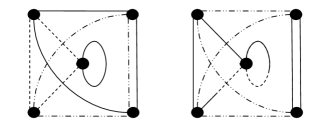
Figure 5: A four-circuit partition $P$ and a three-circuit partition $P^{\prime}$.

In Figure 5, we see two circuit partitions in $F$; $P$ corresponds to the set of four words $\{e,ade,abc,bcd\}$ and $P^{\prime}$ corresponds to $\{aeed,bc,abcd\}$. (In order to trace a circuit in the figure, maintain the dash pattern while traversing each vertex. Note however that the dash pattern may change in the middle of an edge; this is done to prevent the same dash pattern from appearing four times at any vertex, as that would confuse the transitions.) $P$ and $P^{\prime}$ have

$$\mathcal{I}_{P}(C)=\begin{pmatrix}0&0&0&0&0\\ 0&1&0&0&0\\ 0&0&0&0&0\\ 0&0&0&1&0\\ 0&0&0&0&0\end{pmatrix}\text{, }\mathcal{I}_{P}(C^{\prime})=\begin{pmatrix}1&0&0&0&0\\ 0&1&1&0&0\\ 0&1&1&0&0\\ 0&0&0&0&0\\ 0&0&0&0&0\end{pmatrix},$$

$$\mathcal{I}_{P^{\prime}}(C)=\begin{pmatrix}0&0&0&0&0\\ 0&1&1&0&0\\ 0&1&1&0&0\\ 0&0&0&1&0\\ 0&0&0&0&1\end{pmatrix}\text{ and }\mathcal{I}_{P^{\prime}}(C^{\prime})=\begin{pmatrix}1&0&0&0&0\\ 0&0&0&0&0\\ 0&0&1&0&0\\ 0&0&0&0&0\\ 0&0&0&0&1\end{pmatrix}.$$

In accordance with the circuit-nullity formula, $\nu(\mathcal{I}_{P}(C))=\nu(\mathcal{I}_{P}(C^{\prime}))=3$ and $\nu(\mathcal{I}_{P^{\prime}}(C))=\nu(\mathcal{I}_{P^{\prime}}(C^{\prime}))=2$. As predicted by Theorem 16, the nullspace of $\mathcal{I}_{P}(C)$ is spanned by the relative core vectors $(0,0,0,0,1)$, $(1,0,0,0,1)$, $(1,0,1,0,0)$ and $(0,0,1,0,0)$. The nullspace of $\mathcal{I}_{P}(C^{\prime})$ is spanned by the relative core vectors $(0,0,0,0,1)$, $(0,0,0,1,1)$, $(0,1,1,0,0)$ and $(0,1,1,1,0)$. The nullspace of $\mathcal{I}_{P^{\prime}}(C)$ is spanned by $(1,0,0,0,0)$, $(0,1,1,0,0)$ and $(1,1,1,0,0)$; and the nullspace of $\mathcal{I}_{P^{\prime}}(C^{\prime})$ is spanned by $(0,0,0,1,0)$, $(0,1,0,0,0)$ and $(0,1,0,1,0)$.

3 Theorem 13

3.1 Modified inverses from local complementation

Theorem 13 concerns the equivalence relation $\sim_{lc}$ on zero-diagonal symmetric matrices generated by simple local complementations $S\mapsto S^{i}$, where $i$ is an arbitrary index. As noted in the introduction, Theorem 13 is related to results of Brijder and Hoogeboom [16, 17, 18], Glantz and Pelillo [26] and Ilyutko [28, 29] regarding an equivalence relation $\sim_{piv}$ on symmetric matrices that is generated by two kinds of operations: (non-simple) local complementations $S\mapsto S_{ns}^{i}$ where the $i^{th}$ diagonal entry is $1$, and edge pivots $S\mapsto S^{ij}$ where the $i^{th}$ and $j^{th}$ diagonal entries are $0$ and the $ij$ and $ji$ entries are $1$. (The reader familiar with the work of Arratia, Bollobás and Sorkin [1, 2, 3] should be advised that the operation they denote $S^{ij}$ differs from this one by interchanging the $i^{th}$ and $j^{th}$ rows and columns.) It is well known that an edge pivot $S^{ij}$ of a symmetric matrix $S$ coincides with two triple simple local complementations, $S^{ij}=((S^{i})^{j})^{i}=((S^{j})^{i})^{j}$. (See [17] for an extension of this familiar equality to set systems.) This description of the pivot is not very useful in connection with $\sim_{piv}$, as the individual local complementations with respect to $i$ and $j$ are “illegal” for $\sim_{piv}$ when the $i^{th}$ and $j^{th}$ diagonal entries are $0$. It is useful for us, though: as non-simple local complementation coincides with simple local complementation off the diagonal, the description of the pivot implies that if $S$ and $T$ are zero-diagonal symmetric matrices, and $S^{\prime}$ and $T^{\prime}$ are symmetric matrices that are (respectively) equal to $S$ and $T$ except for diagonal entries, then $S^{\prime}\sim_{piv}T^{\prime}\Rightarrow S\sim_{lc}T$.

This implication allows us to prove half of Theorem 13 using a result noted in [16, 17, 18, 26], namely that symmetric matrices related by the principal pivot transform are also related by $\sim_{piv}$. Suppose $S_{1}$ is a zero-diagonal symmetric matrix and $S_{2}$ is a modified inverse of $S_{1}$. Then there are nonsingular symmetric matrices $S_{1}^{\prime}$ and $S_{2}^{\prime}$ that are (respectively) equal to $S_{1}$ and $S_{2}$ except for diagonal entries, and have $(S_{1}^{\prime})^{-1}=S_{2}^{\prime}$. As inverses, $S_{1}^{\prime}$ and $S_{2}^{\prime}$ are related by the principal pivot transform, so $S_{1}^{\prime}\sim_{piv}S_{2}^{\prime}$; consequently the implication of the last paragraph tells us that $S_{1}\sim_{lc}S_{2}$. Iterating this argument, we conclude that $S\sim_{mi}T\Rightarrow S\sim_{lc}T$.

3.2 A brief discussion of the principal pivot transform

The principal pivot transform (ppt) was introduced by Tucker [49]; a survey of its properties was given by Tsatsomeros [48]. The reader who would like to learn about the ppt and its relationship with graph theory should consult these papers, the work of Brijder and Hoogeboom [16, 17, 18] and Glantz and Pelillo [26], and the references given there. For the convenience of the reader who simply wants to understand the argument above, we sketch the details briefly.

The principal pivot transform is valuable for us because it provides a way to obtain the inverse of a nonsingular symmetric $GF(2)$-matrix incrementally, using pivots and non-simple local complementations. This property is not immediately apparent from the definition:

Definition 22

Suppose

$$M=\begin{pmatrix}P&Q\\ R&S\end{pmatrix}$$

is an $n\times n$ matrix with entries in a field $F$, and suppose $P$ is a nonsingular principal submatrix involving the rows and columns whose indices lie in a set $X$. Then

$$M\ast X=\begin{pmatrix}P^{-1}&-P^{-1}Q\\ RP^{-1}&S-RP^{-1}Q\end{pmatrix}.$$

In particular, if $M$ is nonsingular then $M\ast\{1,...,n\}=M^{-1}$.

The matrix $M$ is displayed in the given form only for convenience; the definition may be applied to any set of indices $X$ whose corresponding principal submatrix $P$ is nonsingular.

A direct calculation (which we leave to the reader) yields an alternative characterization: if we think of $F^{n}$ as the direct sum of a subspace corresponding to indices from $X$ and a subspace corresponding to the rest of the indices, then the linear endomorphism of $F^{n}$ corresponding to $M\ast X$ is related to the linear endomorphism corresponding to $M$ by the relation

$$M\begin{pmatrix}x_{1}\\ x_{2}\end{pmatrix}=\begin{pmatrix}y_{1}\\ y_{2}\end{pmatrix}\text{ if and only if }(M\ast X)\begin{pmatrix}y_{1}\\ x_{2}\end{pmatrix}=\begin{pmatrix}x_{1}\\ y_{2}\end{pmatrix}.$$

This characterization directly implies two useful properties.

(1) Suppose $X_{1}$ and $X_{2}$ are subsets of $\{1,...,n\}$, and $(M\ast X_{1})\ast X_{2}$ is defined. Then $M\ast(X_{1}\Delta X_{2})$ is also defined, and it is the same as $(M\ast X_{1})\ast X_{2}$. (Here $\Delta$ denotes the symmetric difference, $X_{1}\Delta X_{2}=(X_{1}\cup X_{2})-(X_{1}\cap X_{2})$.)

(2) If $M$ is nonsingular then the submatrix  $S-RP^{-1}Q$ of $M\ast X$ must be nonsingular too. For

$$(M\ast X)\begin{pmatrix}\mathbf{0}\\ x_{2}\end{pmatrix}=\begin{pmatrix}x_{1}\\ \mathbf{0}\end{pmatrix}\text{ implies }M\begin{pmatrix}x_{1}\\ x_{2}\end{pmatrix}=\begin{pmatrix}\mathbf{0}\\ \mathbf{0}\end{pmatrix},$$

which requires $x_{1}=\mathbf{0}$ and $x_{2}=\mathbf{0}$.

Note also that if $M$ is a symmetric $GF(2)$-matrix, then so is $M\ast X$.

Suppose now that $M$ is a nonsingular symmetric $GF(2)$-matrix. We begin a recursive calculation by performing principal pivot transforms $\ast\{i_{1}\},\ast\{i_{2}\}$, …, $\ast\{i_{k}\}$ for as long as we can, subject to the proviso that $i_{1}$, …, $i_{k}$ are pairwise distinct. It is a direct consequence of Definition 22 that each transformation $\ast\{i_{j}\}$ is the same as non-simple local complementation with respect to $i_{j}$, because $P^{-1}$ is the $1\times 1$ matrix $(1)$, $R$ is the transpose of $Q$, and an entry of $RQ$ is $1$ if and only if its row and column correspond to nonzero entries of $R$ and $Q$. For convenience we display the special case $\{i_{1},...,i_{k}\}=\{1,...,k\}$:

$$M\ast\{i_{1},...,i_{k}\}=M\ast\{i_{1}\}\ast\cdots\ast\{i_{k}\}=M^{\prime}=\begin{pmatrix}P^{\prime}&Q^{\prime}\\ R^{\prime}&S^{\prime}\end{pmatrix},$$

where the diagonal entries of $P^{\prime}$ (resp. $S^{\prime}$) are all $1$ (resp. all $0$) and $R^{\prime}$ is the transpose of $Q^{\prime}.$ Note that by property (2), $S^{\prime}$ is nonsingular; hence each row of $S^{\prime}$ must certainly contain a nonzero entry. Consequently we may (again for convenience) display the matrix in a different way:

$$M\ast\{i_{1},...,i_{k}\}=M^{\prime}=\begin{pmatrix}P^{\prime\prime}&Q^{\prime\prime}\\ R^{\prime\prime}&S^{\prime\prime}\end{pmatrix}\text{ where }P^{\prime\prime}=\begin{pmatrix}0&1\\ 1&0\end{pmatrix}.$$

The next step in the calculation is to perform the principal pivot transform $\ast\{i_{k+1},i_{k+2}\}$, where $i_{k+1}$ and $i_{k+2}$ are the indices involved in $P^{\prime\prime}$. A direct calculation using Definition 22 shows that

$$M^{\prime}\ast\{i_{k+1},i_{k+2}\}=M^{\prime\prime}=\begin{pmatrix}P^{\prime\prime}&Q^{\prime\prime\prime}\\ R^{\prime\prime\prime}&S^{\prime\prime}+X\end{pmatrix}$$

where $Q^{\prime\prime\prime}$ is obtained by interchanging the two rows of $Q^{\prime\prime}$, $R^{\prime\prime\prime}$ is the transpose of $Q^{\prime\prime\prime}$, and $X$ is the matrix whose $ij$ entry is

$$(R^{\prime\prime})_{ii_{k+1}}(Q^{\prime\prime})_{i_{k+2}j}+(R^{\prime\prime})_{ii_{k+2}}(Q^{\prime\prime})_{i_{k+1}j}=(Q^{\prime\prime})_{i_{k+1}i}(Q^{\prime\prime})_{i_{k+2}j}+(Q^{\prime\prime})_{i_{k+2}i}(Q^{\prime\prime})_{i_{k+1}j}.$$

That is, $X_{ij}=0$ unless the $i^{th}$ and $j^{th}$ columns of $Q^{\prime\prime}$ are distinct nonzero vectors. It follows that $M^{\prime\prime}$ is the pivot $(M^{\prime})^{i_{k+1}i_{k+2}}$; equivalently, $M^{\prime\prime}$ is the triple simple local complement $(((M^{\prime})^{i_{k+1}})^{i_{k+2}})^{i_{k+1}}$.

The resulting matrix $M^{\prime\prime}$ has no new nonzero diagonal entry, so the second step may be repeated as many times as necessary. At no point do we re-use an index that has already been involved in a principal pivot transform, at no point do we obtain a non-symmetric matrix, and at no point is the principal submatrix determined by the as-yet unused indices singular. Consequently the calculation proceeds until every index has been involved in precisely one principal pivot transform. By property (1), at the end of the calculation we have obtained $M\ast\{1,...,n\}=M^{-1}$ using individual steps each of which is either a non-simple local complementation or a pivot.

3.3 The $\nu,\nu,\nu+1$ lemma

Lemma 2 of Balister, Bollobás, Cutler and Pebody [4] is a very useful result about the nullities of three related matrices, which we cite in the next section. Here is a sharpened form of the lemma, involving the nullspaces of the three matrices rather than only their nullities.

Lemma 23

Suppose $M$ is a symmetric $GF(2)$-matrix. Let $\rho$ be an arbitrary row vector, and let $\mathbf{0}$ be the row vector with all entries $0$; denote their transposes $\kappa$ and $\mathbf{0}$ respectively. Let $M_{1},M_{2}$ and $M_{3}$ denote the indicated symmetric matrices.

$$M_{1}=\begin{pmatrix}M&\kappa\\ \rho&1\end{pmatrix}\quad\quad M_{2}=\begin{pmatrix}M&\kappa\\ \rho&0\end{pmatrix}\quad\quad M_{3}=\begin{pmatrix}M&\mathbf{0}\\ \mathbf{0}&1\end{pmatrix}$$

Then two of $M_{1},M_{2},M_{3}$ have the same nullspace, say of dimension $\nu$. The nullspace of the remaining matrix has dimension $\nu+1$, and it contains the nullspace shared by the other two.

Proof. We use $rk(N)$ and $\nu(N)$ to denote the rank and nullity of a matrix $N$, $\operatorname{row}(N)$ and $\operatorname{col}(N)$ to denote the spaces spanned by the rows and columns of $N$, and $\ker N$ to denote the nullspace of $N$, i.e., the space of row vectors $x$ with $x\cdot N=\mathbf{0}$.

Case 1. Suppose $\rho\notin\operatorname{row}(M)$; then also $\kappa\notin\operatorname{col}(M)$.

Observe that $\nu(M_{1})=\nu(M_{2})=\nu(M_{3})-1=\nu(M)-1$ in this case.

We claim that $\ker M_{3}\supseteq(\ker M_{1})\cap(\ker M_{2})$. Note first that no row vector $\begin{pmatrix}y&1\end{pmatrix}$ can be an element of both $\ker M_{1}$ and $\ker M_{2}$, because $\begin{pmatrix}y&1\end{pmatrix}\cdot M_{1}=\mathbf{0}\Rightarrow y\cdot\kappa=1$ and $\begin{pmatrix}y&1\end{pmatrix}\cdot M_{2}=\mathbf{0}\Rightarrow y\cdot\kappa=0$. Consequently every $x\in(\ker M_{1})\cap(\ker M_{2})$ is of the form $\begin{pmatrix}y&0\end{pmatrix}$ for some $y\in\ker M$. Obviously

$$\ker M_{3}=\left\{\begin{pmatrix}y&0\end{pmatrix}\text{ $|$ }y\in\ker M\right\},$$

so the claim is verified.

The inclusion

$$(\ker M_{1})\cap(\ker M_{2})\supseteq\left\{\begin{pmatrix}y&0\end{pmatrix}\text{ $|$ }y\in\ker M\text{ and }y\cdot\kappa=0\right\}$$

is obvious, but note that the dimension of the right hand side is at least $\nu(M)-1$. As $\nu(M)-1=\nu(M_{1})=\nu(M_{2})$, we conclude that

$$\ker M_{1}=\ker M_{2}=(\ker M_{1})\cap(\ker M_{2})=\left\{\begin{pmatrix}y&0\end{pmatrix}\text{ $|$ }y\in\ker M\text{ and }y\cdot\kappa=0\right\}.$$

Case 2. Suppose $\rho\in\operatorname{row}(M)$; then also $\kappa\in\operatorname{col}(M)$.

As $\rho\in\operatorname{row}(M)$, at least one of $\begin{pmatrix}\rho&0\end{pmatrix},\begin{pmatrix}\rho&1\end{pmatrix}$ is an element of $\operatorname{row}\begin{pmatrix}M&\kappa\end{pmatrix}$. If both are elements then

$$rk\begin{pmatrix}M&\kappa\end{pmatrix}=rk\begin{pmatrix}M&\kappa\\ \rho&0\\ \rho&1\end{pmatrix}=rk\begin{pmatrix}M&\kappa\\ \rho&0\\ \mathbf{0}&1\end{pmatrix}=rk\begin{pmatrix}M&\mathbf{0}\\ \rho&0\\ \mathbf{0}&1\end{pmatrix}=rk(M)+1$$

and hence $\kappa\notin\operatorname{col}(M)$, an impossibility. Consequently one of $M_{1},M_{2}$ is of rank $rk(M)$, and the other is of rank $rk(M)+1=rk(M_{3})$.

We claim that $\ker M_{3}\subseteq(\ker M_{1})\cap(\ker M_{2})$. Suppose $x\in\ker M_{3}$; clearly then $x=\begin{pmatrix}y&0\end{pmatrix}$ for some $y\in\ker M$. As $y\in\ker M$, $y\cdot z=0$ $\forall z\in\operatorname{col}(M)$. It follows that $y\cdot\kappa=0$, and hence $x\in(\ker M_{1})\cap(\ker M_{2})$ as claimed.

As one of $M_{1},M_{2}$ has nullity $\nu(M_{3})$ and the other has nullity $\nu(M_{3})+1$, the claim implies that either $\ker M_{3}=\ker M_{2}\subset\ker M_{1}$ or $\ker M_{3}=\ker M_{1}\subset\ker M_{2}$.   

3.4 Local complements from modified inversion

The implication $S\sim_{lc}T\Rightarrow S\sim_{mi}T$ does not follow directly from results regarding $\sim_{piv}$, but our argument uses two lemmas very similar to ones used by Ilyutko [28].

Lemma 24

Let $S$ be an $n\times n$ zero-diagonal symmetric $GF(2)$-matrix. Suppose $1\leq i\leq n$ and the $i^{th}$ row of $S$ has at least one nonzero entry. Then there is a nonsingular symmetric $GF(2)$-matrix $M$ that differs from $S$ only in diagonal entries other than the $i^{th}$.

Proof. We may as well presume that $i=1$, and that $s_{12}\neq 0$.

For $k\geq 2$ let $S_{k}$ be the submatrix of $S$ obtained by deleting all rows and columns with indices $>k$. We claim that for every $k\geq 2$, there is a subset $T_{k}\subseteq\{3,...,k\}$ with the property that we obtain a nonsingular matrix $S_{k}^{\prime}$ by toggling the diagonal entries of $S_{k}$ with indices in $T_{k}$. When $k=2$ the claim is satisfied by $T_{2}=\emptyset.$

Proceeding inductively, suppose $k\geq 2$ and $T_{k}\subseteq\{3,...,k\}$ satisfies the claim. If we obtain a nonsingular matrix by toggling the diagonal entries of $S_{k+1}$ with indices in $T_{k}$, then $T_{k+1}=T_{k}$ satisfies the claim for $k+1$. If not, then the $\nu,\nu,\nu+1$ lemma implies that $T_{k+1}=T_{k}\cup\{k+1\}$ satisfies the claim.

The required matrix $M$ is obtained from $S=S_{n}$ by toggling the diagonal entries with indices in $T_{n}$.   

Lemma 25

Suppose

$$M=\begin{pmatrix}0&\mathbf{1}&\mathbf{0}\\ \mathbf{1}&M_{11}&M_{12}\\ \mathbf{0}&M_{12}&M_{22}\end{pmatrix}$$

is a nonsingular symmetric matrix, with

$$M^{-1}=\begin{pmatrix}a&\rho\\ \kappa&N\end{pmatrix}.$$

Then the matrix

$$M^{\prime}=\begin{pmatrix}0&\mathbf{1}&\mathbf{0}\\ \mathbf{1}&\bar{M}_{11}&M_{12}\\ \mathbf{0}&M_{12}&M_{22}\end{pmatrix}$$

obtained by toggling all entries within the block $M_{11}$ is also nonsingular, and

$$(M^{\prime})^{-1}=\begin{pmatrix}a+1&\rho\\ \kappa&N\end{pmatrix}.$$

Proof. $M^{-1}\cdot M$ is the identity matrix, so

$$\begin{pmatrix}a&\rho\end{pmatrix}\cdot\begin{pmatrix}0\\ \mathbf{1}\\ \mathbf{0}\end{pmatrix}=1\text{;}$$

consequently the row vector $\rho$ must have an odd number of nonzero entries in the columns corresponding to the $\mathbf{1}$ in the first row of $M$. Similarly, each row of $N$ must have an even number of nonzero entries in these columns, because

$$\begin{pmatrix}\kappa&N\end{pmatrix}\cdot\begin{pmatrix}0\\ \mathbf{1}\\ \mathbf{0}\end{pmatrix}=\mathbf{0}.$$

It follows that the products

$$\begin{pmatrix}a&\rho\\ \kappa&N\end{pmatrix}\cdot M\text{ and }\begin{pmatrix}a+1&\rho\\ \kappa&N\end{pmatrix}\cdot M^{\prime}$$

are equal.   

As stated, Lemma 25 requires that the first row of $M$ be in the form $\begin{pmatrix}0&\mathbf{1}&\mathbf{0}\end{pmatrix}$. This is done only for convenience; the general version of the lemma applies to any row in which the diagonal entry is $0$.

Suppose now that $S$ is a zero-diagonal symmetric $n\times n$ matrix and $1\leq i\leq n$. If every entry of the $i^{th}$ row of $S$ is $0$, then the local complement $S^{i}$ is the same as $S$.

If the $i^{th}$ row of $S$ includes some nonzero entry, then Lemma 24 tells us that there is a nonsingular matrix $M$ such that (a) $M$ is obtained from $S$ by toggling some diagonal entries other than the $i^{th}$. The general version of Lemma 25 then tells us that there is a nonsingular matrix $M^{\prime}$ such that (b) $(M^{\prime})^{-1}$ equals $M^{-1}$ except for the $i^{th}$ diagonal entry and (c) $M^{\prime}$ equals the local complement $S^{i}$ except for diagonal entries. Condition (a) implies that a modified inverse $T$ of $S$ is obtained by changing all diagonal entries of $M^{-1}$ to $0$; condition (b) implies that $T$ is also equal to $(M^{\prime})^{-1}$ except for diagonal entries; and condition (c) implies that the local complement $S^{i}$ is a modified inverse of $T$.

It follows that every simple local complement $S^{i}$ can be obtained from $S$ using no more than two modified inversions. Applying this repeatedly, we conclude that $S\sim_{lc}T\Rightarrow S\sim_{mi}T$.

4 Theorem 16

Let $F$ be a 4-regular multigraph with an Euler system $C$, and suppose $v\in V(F)$. Let the Euler circuit of $C$ incident at $v$ be $vC_{1}vC_{2}v$, where $v$ does not appear within $C_{1}$ or $C_{2}$. Every edge of the connected component of $F$ that contains $v$ lies on precisely one of $C_{1},C_{2}$. If $w\neq v$ is a vertex of this component which is not a neighbor of $v$ in $\mathcal{I}(C)$, i.e., $v$ and $w$ are not interlaced with respect to $C$, then all four half-edges incident at $w$ appear on the same $C_{i}$. On the other hand, if $v$ and $w$ are neighbors in $\mathcal{I}(C)$ then two of the four half-edges incident at $w$ appear on $C_{1}$, and the other two appear on $C_{2}$. Moreover the only transition at $w$ that pairs together the half-edges from the same $C_{i}$ is the $\phi$ transition; the $\chi$ and $\psi$ transitions at $w$ pair each half-edge from $C_{1}$ with a half-edge from $C_{2}$. At $v$, instead, only the $\chi$ transition pairs together half-edges from the same $C_{i}$; the $\phi$ and $\psi$ transitions pair each half-edge from $C_{1}$ with a half-edge from $C_{2}$. These observations are summarized in the table below, where $N(v)$ denotes the set of neighbors of $v$ in $\mathcal{I}(C)\,$, $(1)(2)$ indicates a transition that pairs together half-edges from the same $C_{i}$ and $(12)$ indicates a transition that pairs each half-edge from $C_{1}$ with a half-edge from $C_{2}$.

	vertex	$v$	$w\in N(v)$	$w\notin N(v)$
transition
$\phi$		$(12)$	$(1)(2)$	$(1)(2)$
$\chi$		$(1)(2)$	$(12)$	$(1)(2)$
$\psi$		$(12)$	$(12)$	$(1)(2)$

Suppose $\gamma$ is a circuit that is singly incident at $v$, and involves the $\phi$ transition at $v$. We start following $\gamma$ at $v$, on a half-edge that belongs to $C_{i}$. We return to $v$ on a half-edge that belongs to $C_{j}$, $j\neq i$, so while following $\gamma$ we must have switched between $C_{i}$ and $C_{j}$ an odd number of times. (See Figure 6.) That is,

$$\left|\{w\in N(v)\text{ $|$ }\gamma\text{ is singly incident at }w\text{ and involves the }\chi\text{ or }\psi\text{ transition at }w\}\right|$$

must be odd.

Figure 6: An Euler circuit and three circuits that are singly incident at a vertex.

Suppose instead that $\gamma$ is a circuit that is singly incident at $v$ and involves the $\chi$ transition at $v$. If we start following $\gamma$ along a half-edge that belongs to $C_{i}$, we must return to $v$ on the other half-edge that belongs to $C_{i}$, so we must have switched between $C_{i}$ and $C_{j}$ an even number of times. Consequently

$$\left|\{w\in N(v)\text{ $|$ }\gamma\text{ is singly incident at }w\text{ and involves the }\chi\text{ or }\psi\text{ transition at }w\}\right|$$

must be even.

Similarly, if $\gamma$ is a circuit that is singly incident at $v$ and involves the $\psi$ transition at $v$ then

$$\left|\{w\in N(v)\text{ $|$ }\gamma\text{ is singly incident at }w\text{ and involves the }\chi\text{ or }\psi\text{ transition at }w\}\right|$$

must be odd.

Suppose $\gamma$ is doubly incident at $v$ and we follow $\gamma$ after leaving $v$ on a half-edge that belongs to $C_{1}$. We cannot be sure on which half-edge we will first return to $v$. But after leaving again, we must return on the one remaining half-edge. If the first return is from $C_{1}$, then on the way we must traverse an even number of vertices $w\in N(v)$ such that $\gamma$ is singly incident at $w$ and involves the $\chi$ or $\psi$ transition at $w$; moreover when we follow the second part of $\gamma$ we will leave $v$ in $C_{2}$ and also return in $C_{2}$, so again we must encounter an even number of such vertices. If the first return is from $C_{2}$ instead, then on the way we must traverse an odd number of vertices $w\in N(v)$ such that $\gamma$ is singly incident at $w$ and involves the $\chi$ or $\psi$ transition at $w$; the second part of the circuit will begin in $C_{i}$ and end in $C_{j}$ ($j\neq i$), so it will also include an odd number of such vertices. In any case,

$$\left|\{w\in N(v)\text{ $|$ }\gamma\text{ is singly incident at }w\text{ and involves the }\chi\text{ or }\psi\text{ transition at }w\}\right|$$

must be even.

Proposition 26

Let $F$ be a 4-regular multigraph with an Euler system $C$, and suppose $P$ is a circuit partition of $F$. Then $\rho(\gamma,C)\in\ker\mathcal{I}_{P}(C)$ $\forall\gamma\in P$.

Proof. Recall that $\rho(\gamma,C)\in GF(2)^{V(F)}$ has nonzero entries corresponding to the vertices where $\gamma$ is singly incident and does not involve the $\phi$ transition; we consider $\rho(\gamma,C)$ as a row vector. Let $v\in V(F)$, and let $\kappa(v)$ be the column of $\mathcal{I}_{P}(C)$ corresponding to $v$.

If $\gamma$ lies in a different connected component than $v$, or if $P$ involves the $\phi$ transition at $v$, then for every $w\in V(F)$ at least one of $\rho(\gamma,C)$ and $\kappa(v)$ has its entry corresponding to $w$ equal to $0$; consequently $\rho(\gamma,C)\cdot\kappa(v)=0$.

If $\gamma$ lies in the same component as $v$ and $P$ involves the $\chi$ transition at $v$, then considering the definitions of $\rho(\gamma,C)$ and $\mathcal{I}_{P}(C)$, we see that $\rho(\gamma,C)\cdot\kappa(v)$ is the mod 2 parity of

$$\left|\{w\in N(v)\text{ $|$ }\gamma\text{ is singly incident at }w\text{ and involves the }\chi\text{ or }\psi\text{ transition at }w\}\right|.$$

Whether $\gamma$ is singly or doubly incident at $v$, this number is even as observed above.

If $\gamma$ lies in the same component as $v$ and $P$ involves the $\psi$ transition at $v$, then considering the definitions of $\rho(\gamma,C)$ and $\mathcal{I}_{P}(C)$, we see that $\rho(\gamma,C)\cdot\kappa(v)$ is the mod 2 parity of this sum:

$$\left|\{w\in N(v)\text{ $|$ }\gamma\text{ is singly incident at }w\text{ and involves the }\chi\text{ or }\psi\text{ transition at }w\}\right|$$

$$+\left\{\begin{tabular}[c]{ll}1,&if $\gamma$ is singly incident at $v$\\ 0,&if $\gamma$ is doubly incident at $v$\end{tabular}\ \ \ \ \ \ \right.$$

Whether $\gamma$ is singly or doubly incident at $v$, the sum is even as observed above.   

Proposition 27

Let $F$ be a 4-regular multigraph with an Euler system $C$, and let $P$ be a circuit partition of $F$. Suppose $Q\subset P$ and there is at least one connected component of $F$ for which $Q$ contains some but not all of the incident circuits of $P$. Then there is at least one vertex $v\in V(F)$ such that $P$ involves the $\chi$ or $\psi$ transition at $v$, precisely one circuit of $Q$ is incident at $v$, and this incident circuit of $Q$ is only singly incident.

Proof. Let $F_{0}$ be a connected component of $F$ in which $Q$ includes some but not all of the incident circuits of $P$. Then there must be an edge of $F_{0}$ not included in any circuit of $Q$.

Choose such an edge, $e_{1}$. If a circuit of $Q$ is incident on an end-vertex of $e_{1}$, then that circuit is only singly incident. If not, choose an edge $e_{2}$ that connects an end-vertex of $e_{1}$ to a vertex that is not incident on $e_{1}$. Continuing this process, we must ultimately find a vertex at which precisely one circuit of $Q$ is incident, and this circuit is only singly incident.

Suppose $P$ involves the $\phi$ transition at every such vertex. Then every circuit of $P$ that is contained in $F_{0}$ and not included in $Q$ involves only $\phi$ transitions. This is impossible, as the only circuit contained in $F_{0}$ that involves only $\phi$ transitions is the Euler circuit of $F_{0}$ included in $C$.   

Corollary 28

Let $F$ be a 4-regular multigraph with an Euler system $C$, and suppose $P$ is a circuit partition of $F$. Suppose $Q\subset P$ and there is no connected component of $F$ for which $Q$ contains every incident circuit of $P$. Then $\{$relative core vectors of the circuits of $Q\}$ is linearly independent.

Proof. If $Q$ is empty then recall that $\emptyset$ is independent by convention. Otherwise, let $Q^{\prime}$ be any nonempty subset of $Q$. Proposition 27 tells us that there is a vertex $v$ of $F$ at which $P$ involves the $\chi$ or $\psi$ transition, precisely one circuit of $Q^{\prime}$ is incident, and this circuit is singly incident. It follows that the $v$ coordinate of

$$\sum_{\gamma\in Q^{\prime}}\rho(\gamma,C)$$

is $1$, and hence

$$\sum_{\gamma\in Q^{\prime}}\rho(\gamma,C)\not=\mathbf{0}\text{.}$$

 

Proposition 26 and Corollary 28 tell us that the relative core vectors of the circuits of a circuit partition $P$ span a $(\left|P\right|-c(F))$-dimensional subspace of $\ker\mathcal{I}_{P}(C)$. The circuit-nullity formula tells us that $\left|P\right|-c(F)$ is the nullity of $\mathcal{I}_{P}(C)$, so we conclude that the relative core vectors span the nullspace of $\mathcal{I}_{P}(C)$.

This completes our proof of Theorem 16. Before proceeding we should recall the work of Jaeger [30], whose Proposition 4 is equivalent to the special case of Theorem 16 in which $P$ involves no $\phi$ transitions. A different way to prove Theorem 16 is to reduce to the special case using detachment [21, 41] along $\phi$ transitions. We prefer the argument above because it avoids the conceptual complications introduced by Jaeger’s use of chord diagrams and surface imbeddings.

5 Theorem 17

Suppose $C$ and $C^{\prime}$ are Euler systems of $F$, and $v\in V(F)$. We use transition labels $\phi,\chi,\psi$ with respect to $C$, and $\phi^{\prime},\chi^{\prime},\psi^{\prime}$ with respect to $C^{\prime}$.

If $C$ and $C^{\prime}$ involve the same transition at $v$, then the row and column of both $\mathcal{I}_{C}(C^{\prime})$ and $\mathcal{I}_{C^{\prime}}(C)$ corresponding to $v$ are the same as those of the identity matrix, so the row and column of $\mathcal{I}_{C}(C^{\prime})\cdot\mathcal{I}_{C^{\prime}}(C)$ corresponding to $v$ are the same as those of the identity matrix.

Suppose instead that $C$ and $C^{\prime}$ involve different transitions at $v$. Then $C^{\prime}$ involves the $\chi$ or the $\psi$ transition, and $C$ involves the $\chi^{\prime}$ or the $\psi^{\prime}$ transition; the four possible combinations are illustrated in Figure 3 of the introduction. N.b. The caption of Figure 3 mentions $C\#W$, but the figure is valid for any Euler circuits that do not involve the same transition at $v$.

Let $vC_{1}vC_{2}v$ be the circuit of $C$ incident at $v$; then $vC_{1}v$ and $vC_{2}v$ are the two circuits obtained by “short-circuiting” $C$ at $v$. We claim that the relative core vector $\rho(vC_{1}v,C^{\prime})$ is the same as the row of $\mathcal{I}_{C^{\prime}}(C)$ corresponding to $v$. The entry of $\rho(vC_{1}v,C^{\prime})$ corresponding to a vertex $w\neq v$ is $1$ if and only if $vC_{1}v$ is singly incident at $w$, and $vC_{1}v$ does not involve the $\phi^{\prime}$ transition at $w$. Also, the $vw$ entry of $\mathcal{I}_{C^{\prime}}(C)$ is $1$ if and only if $v$ and $w$ are interlaced with respect to $C$, and $C^{\prime}$ does not involve the $\phi$ transition at $w$. As $vC_{1}v$ and $C$ both involve the $\phi$ transition at every $w\neq v$, the two entries are the same. On the other hand, the entry of $\rho(vC_{1}v,C^{\prime})$ corresponding to $v$ is $1$ unless the transition of $vC_{1}v$ at $v$ (that is, the $\chi$ transition) is the $\phi^{\prime}$ transition, and the $vv$ entry of $\mathcal{I}_{C^{\prime}}(C)$ is $1$ unless the transition of $C^{\prime}$ at $v$ (the $\phi^{\prime}$ transition) is the $\chi$ transition. These two entries are also the same, so $\rho(vC_{1}v,C^{\prime})$ is indeed the same as the row of $\mathcal{I}_{C^{\prime}}(C)$ corresponding to $v$.

It follows that $\rho(vC_{1}v,C^{\prime})\cdot\mathcal{I}_{C}(C^{\prime})$ is the row of $\mathcal{I}_{C^{\prime}}(C)\cdot\mathcal{I}_{C}(C^{\prime})$ corresponding to $v$. We claim that this coincides with the corresponding row of the identity matrix, i.e., if $w\in V(F)$ and $\kappa_{w}$ is the column of $\mathcal{I}_{C}(C^{\prime})$ corresponding to $w$ then $\rho(vC_{1}v,C^{\prime})\cdot\kappa_{w}=1$ if and only if $w=v$.

Let $P(C,v)$ be the circuit partition that includes $vC_{1}v$ and $vC_{2}v$, along with all the circuits of $C$ not incident at $v$. Alternatively, we may describe $P(C,v)$ as the circuit partition that involves $\phi$ transitions at vertices than $v$, and involves the $\chi$ transition at $v$. As $C$ and $P(C,v)$ involve the same transitions at vertices other than $v$, the relative interlacement matrices $\mathcal{I}_{C}(C^{\prime})$ and $\mathcal{I}_{P(C,v)}(C^{\prime})$ coincide except for the row and column corresponding to $v$. Looking at Figure 3, we see that in the cases $\chi\psi^{\prime}$ and $\chi\chi^{\prime}$, $P(C,v)$ involves the $\phi^{\prime}$ transition at $v$; in the case $\psi\psi^{\prime}$,$\ P(C,v)$ involves the $\chi^{\prime}$ transition at $v$; and in the case $\psi\chi^{\prime}$, $P(C,v)$ involves the $\psi^{\prime}$ transition at $v$.

Consider the cases $\chi\psi^{\prime}$ and $\chi\chi^{\prime}$. If $w\neq v$ then the column $\kappa_{w}$ of $\mathcal{I}_{C}(C^{\prime})$ is the same as the column of $\mathcal{I}_{P(C,v)}(C^{\prime})$ corresponding to $w$, except for the entry corresponding to $v$; changing this entry does not affect $\rho(vC_{1}v,C^{\prime})\cdot\kappa_{w}$, because $P(C,v)$ involves the $\phi^{\prime}$ transition at $v$ and hence the entry of $\rho(vC_{1}v,C^{\prime})$ corresponding to $v$ is $0$. Consequently Theorem 16 tells us that $\rho(vC_{1}v,C^{\prime})\cdot\kappa_{w}=0$. Theorem 16 also tells us that $\rho(vC_{1}v,C^{\prime})\neq\mathbf{0}$; as $\mathcal{I}_{C}(C^{\prime})$ is nonsingular, it follows that $\rho(vC_{1}v,C^{\prime})\cdot\kappa_{v}=1.$

Now consider the cases $\psi\psi^{\prime}$ and $\chi\chi^{\prime}$. The only vertex at which $C$ and $P(C,v)$ involve different transitions is $v$, where one involves the $\chi^{\prime}$ transition and the other involves the $\psi^{\prime}$ transition; consequently $\mathcal{I}_{P(C,v)}(C^{\prime})$ and $\mathcal{I}_{C}(C^{\prime})$ coincide except for their $vv$ entries, which are opposites. The entry of $\rho(vC_{1}v,C^{\prime})$ corresponding to $v$ is $1$, so $\rho(vC_{1}v,C^{\prime})\cdot\mathcal{I}_{P(C,v)}(C^{\prime})=\mathbf{0}$ tells us that $\rho(vC_{1}v,C^{\prime})\cdot\kappa_{v}\neq 0$, and $\rho(vC_{1}v,C^{\prime})\cdot\kappa_{w}=0$ for $w\neq v$.

The closing comment of the last section applies here too: the special case of Theorem 17 involving compatible Euler systems follows from Jaeger’s proof of Proposition 5 of [30], and the general case may be reduced to the special case by detachment.

Acknowledgments. We would like to thank R. Brijder and D. P. Ilyutko for many enlightening conversations. The final version of the paper also profited from the careful attention of two anonymous readers.

References

- [1] R. Arratia, B. Bollobás, G. B. Sorkin, The interlace polynomial: A new graph polynomial, in: Proceedings of the Eleventh Annual ACM-SIAM Symposium on Discrete Algorithms (San Francisco, CA, 2000), ACM, New York, 2000, pp. 237-245.
- [2] R. Arratia, B. Bollobás, G. B. Sorkin, The interlace polynomial of a graph, J. Combin. Theory Ser. B 92 (2004) 199-233.
- [3] R. Arratia, B. Bollobás, G. B. Sorkin, A two-variable interlace polynomial, Combinatorica 24 (2004) 567-584.
- [4] P. N. Balister, B. Bollobás, J. Cutler, L. Pebody, The interlace polynomial of graphs at -1, European J. Combin. 23 (2002) 761-767.
- [5] I. Beck, Cycle decomposition by transpositions, J. Combin. Theory Ser. A 23 (1977) 198-207.
- [6] I. Beck, G. Moran, Introducing disjointness to a sequence of transpositions, Ars. Combin. 22 (1986) 145-153.
- [7] A. Bouchet, Caractérisation des symboles croisés de genre nul, C. R. Acad. Sci. Paris Sér. A-B 274 (1972) A724-A727.
- [8] A. Bouchet, Unimodularity and circle graphs, Discrete Math. 66 (1987) 203-208.
- [9] A. Bouchet, Reducing prime graphs and recognizing circle graphs, Combinatorica 7 (1987) 243-254.
- [10] A. Bouchet, Circle graph obstructions, J. Combin. Theory Ser. B 60 (1994) 107-144.
- [11] A. Bouchet, Multimatroids. I. Coverings by independent sets, SIAM J. Discrete Math. 10 (1997) 626-646.
- [12] A. Bouchet, Multimatroids. II. Orthogonality, minors and connectivity, Electron. J. Combin. 5 (1998) #R8.
- [13] A. Bouchet, Multimatroids III. Tightness and fundamental graphs, European J. Combin. 22 (2001) 657-677.
- [14] A. Bouchet, Multimatroids. IV. Chain-group representations, Linear Algebra Appl. 277 (1998) 271-289.
- [15] H. R. Brahana, Systems of circuits on two-dimensional manifolds, Ann. Math. 23 (1921) 144-168.
- [16] R. Brijder, H. J. Hoogeboom, Maximal pivots on graphs with an application to gene assembly, Discrete Appl. Math. 158 (2010) 1977-1985.
- [17] R. Brijder, H. J. Hoogeboom, The group structure of pivot and loop complementation on graphs and set systems, European J. Combin., to appear.
- [18] R. Brijder, H. J. Hoogeboom, Nullity invariance for pivot and the interlace polynomial, Linear Algebra Appl. 435 (2011) 277-288.
- [19] M. Cohn, A. Lempel, Cycle decomposition by disjoint transpositions, J. Combin. Theory Ser. A 13 (1972) 83-89.
- [20] J. A. Ellis-Monaghan, I. Sarmiento, Generalized transition polynomials, Congr. Numer. 155 (2002) 57-69.
- [21] H. Fleischner, Eulerian graphs and related topics. Part 1. Vol. 1. Annals of Discrete Mathematics, 45. North-Holland Publishing Co., Amsterdam, 1990.
- [22] H. Fleischner, Eulerian graphs and related topics. Part 1. Vol. 2. Annals of Discrete Mathematics, 50. North-Holland Publishing Co., Amsterdam, 1991.
- [23] H. de Fraysseix, A characterization of circle graphs, European J. Combin. 5 (1984) 223-238.
- [24] F. Genest, Graphes eulériens et complémentarité locale, Ph. D. Thesis, Université de Montréal, 2001.
- [25] F. Genest, Circle graphs and the cycle double cover conjecture, Discrete Math. 309 (2009) 3714-3725.
- [26] R. Glantz, M. Pelillo, Graph polynomials from principal pivoting, Discrete Math. 306 (2006) 3253-3266.
- [27] C. Godsil, G. Royle, Algebraic Graph Theory, Springer-Verlag, Berlin, Heidelberg and New York (2001).
- [28] D. P. Ilyutko, Framed 4-valent graphs: Euler tours, Gauss circuits and rotating circuits, Mat. Sb., to appear.
- [29] D. P. Ilyutko, An equivalence between the set of graph-knots and the set of homotopy classes of looped graphs, J. Knot Theory Ramifications, to appear.
- [30] F. Jaeger, On some algebraic properties of graphs, in: Progress in graph theory (Waterloo, Ont., 1982), Academic Press, Toronto, 1984, pp. 347-366.
- [31] F. Jaeger, On transition polynomials of 4-regular graphs, in: Cycles and rays (Montreal, PQ, 1987), NATO Adv. Sci. Inst. Ser. C Math. Phys. Sci., 301, Kluwer Acad. Publ., Dordrecht, 1990, pp. 123-150.
- [32] J. Jonsson, On the number of Euler trails in directed graphs, Math. Scand. 90 (2002) 191-214.
- [33] J. Keir, R. B. Richter, Walks through every edge exactly twice II, J. Graph Theory 21 (1996) 301-309.
- [34] A. Kotzig, Eulerian lines in finite 4-valent graphs and their transformations, in: Theory of Graphs (Proc. Colloq., Tihany, 1966), Academic Press, New York, 1968, pp. 219-230.
- [35] M. Las Vergnas, Le polynôme de Martin d’un graphe Eulérien, Ann. Discrete Math. 17 (1983) 397-411.
- [36] J. Lauri, On a formula for the number of Euler trails for a class of digraphs, Discrete Math. 163 (1997) 307-312.
- [37] N. Macris, J. V. Pulé, An alternative formula for the number of Euler trails for a class of digraphs, Discrete Math. 154 (1996) 301-305.
- [38] P. Martin, Enumérations eulériennes dans les multigraphes et invariants de Tutte-Grothendieck, Thèse, Grenoble (1977).
- [39] B. Mellor, A few weight systems arising from intersection graphs, Michigan Math. J. 51 (2003) 509-536.
- [40] G. Moran, Chords in a circle and linear algebra over GF(2), J. Combin. Theory Ser. A 37 (1984) 239-247.
- [41] C. St. J. A. Nash-Williams, Acyclic detachments of graphs, in: Graph theory and combinatorics (Proc. Conf., Open Univ., Milton Keynes, 1978), Res. Notes in Math., 34, Pitman, Boston, 1979, pp. 87–97.
- [42] R. C. Read, P. Rosenstiehl, On the Gauss crossing problem, in: Combinatorics (Proc. Fifth Hungarian Colloq., Keszthely, 1976), Vol. II, Colloq. Math. Soc. János Bolyai, 18, North-Holland, Amsterdam-New York, 1978, pp. 843-876.
- [43] R. B. Richter, Walks through every edge exactly twice, J. Graph Theory 18 (1994) 751-755.
- [44] E. Soboleva, Vassiliev knot invariants coming from Lie algebras and 4-invariants, J. Knot Theory Ramifications 10 (2001) 161-169.
- [45] S. Stahl, On the product of certain permutations, European J. Combin. 8 (1987) 69-72.
- [46] L. Traldi, Binary nullity, Euler circuits and interlacement polynomials, European J. Combin. 32 (2011) 944-950.
- [47] L. Traldi, On the interlace polynomials, preprint: arXiv:1008.0091v4.
- [48] M. J. Tsatsomeros, Principal pivot transforms: properties and applications, Linear Alg. Appl. 307 (2000) 151–165.
- [49] A. W. Tucker, A combinatorial equivalence of matrices, in: Combinatorial Analysis (Proc. Symposia Appl. Math., Vol. X), Amer. Math. Soc., Providence, 1960, pp. 129-140.
- [50] L. Zulli, A matrix for computing the Jones polynomial of a knot, Topology 34 (1995) 717-729.