Hearing shapes of drums — mathematical and physical aspects of isospectrality

Abstract

In a celebrated paper “Can one hear the shape of a drum?” M. Kac [Amer. Math. Monthly 73, 1 (1966)] asked his famous question about the existence of nonisometric billiards having the same spectrum of the Laplacian. This question was eventually answered positively in 1992 by the construction of noncongruent planar isospectral pairs. This review highlights mathematical and physical aspects of isospectrality.

I Introduction

Elastic plates are probably some of the oldest supports of sound production. They were used by most human cultures. Clay drums dated from the Chalcolithic have been found in graves in central Europe, and bronze drums dated from the second millenary B.C. have been discovered in Sweden and Hungary. However, it is usually acknowledged that the scientific study of the vibration of elastic plates goes back only to the end of the 18th century, when the German researcher Ernst Chladni carried out the first systematic investigations on the production of sound by plates Chladni (1802); Smilansky and Stöckmann (2007). When the plate was fixed in its middle and struck with a bow, it was set into vibration. The mode that was being excited was physically visualized by pouring sand on the plate: the sand accumulates at nodal lines, that is lines along which the plate does not oscillate. Some insight was brought into the mathematical theory of vibrating plates by the French mathematician Sophie Germain, who published Recherches sur la théorie des surfaces élastiques in 1821. In the course of the 19th century, Poisson, Kirchhoff, Lamé, Mathieu, and Clebsch, devised analytic expressions for the description of the oscillation for elementary shapes such as the rectangle, the triangle, the circle, and the ellipse.

The motivation for studying this problem was mainly that the wave phenomenon at the heart of membrane oscillations is in fact quite general. The stationary wave equation describing the problem arises in a variety of situations. In many fields of physics, such as acoustics, seismology, hydrodynamics, and heat propagation, the mathematical formulation of the problem involves partial differential equations, and general solutions of these equations can be found as superpositions of solutions of the so-called Helmholtz equation. In a $d$-dimensional space a stationary solution to the wave equation is an unknown function of $d$ variables describing the problem, and the Helmholtz equation reads

$$\Delta f+Ef=0,$$ (1)

where $\Delta$ is the $d$-dimensional Laplacian. Under suitable approximations, numerous problems can be cast in that form. For instance, in a certain regime the oscillations of the height $f=f(x,y)$ of a thin vibrating plate at point $(x,y)$ can be described by (1).

At the end of the 19th century, James C. Maxwell showed that the electric and the magnetic field behave like waves and established equations governing the time evolution of the electromagnetic field. From Maxwell’s equations it is easy to prove that the electric and the magnetic field components also obey the same wave equation (1). Further interest developed in this equation when the wave-like behavior of matter was discovered in the early years of quantum mechanics. The Schrödinger equation was established in 1926 by Erwin Schrödinger to describe the spacetime evolution of a quantum system. The behavior of a particle can be described, in the framework of quantum mechanics, by a wave function $\psi$, which is a function of the position of the particle, and which characterizes the probability amplitude $\psi(x)$ that the particle be located at a position $x$. If the system is described by the Hamiltonian $H$, the wave function satisfies the stationary Schrödinger equation $H\Psi=E\Psi$, where $E$ is the energy of the particle. For a particle of mass $m$ and momentum $p$ evolving in a box defined by its contour $\partial B$, the Hamiltonian describing the free motion inside the box reads $H=p^{2}/2m$ inside the box enclosure $\partial B$ and $\infty$ outside, and the time-independent Schrödinger equation takes the form (1).

Mathematically, solutions of the Helmholtz equation are readily obtained in dimension $d=1$. The problem of vibrating strings had been solved in the 18th century by Jean Le Rond d’Alembert. For a string of length $L$ fixed at its two ends, solutions are simply given by $f(x)=\sin(n\pi x/L)$, where $n$ is an integer. The sound produced by the string has the possible frequencies $n\nu_{0}$, with the fundamental frequency given by $\nu_{0}=c/(2L)$.

Just as the one-dimensional case — which can describe a variety of physical situations — can be seen as a problem of vibrating strings, the two-dimensional case is usually studied from the perspective of its simplest mathematical equivalent, namely billiards. Billiards (in the mathematical sense) are two-dimensional compact domains of the Euclidean plane $\mathbb{R}^{2}$. For instance, in quantum mechanics, the billiard models the behavior of a particle moving freely in a box whose dimensions are such that it can be approximated by a two-dimensional enclosure. The billiard problem is solved by looking for eigenfunctions $\psi$ and eigenvalues $E$ that are solutions of Eq. (1) inside the billiard, imposing boundary conditions on the boundary $\partial B$ of the billiard. Physical problems impose specific boundary conditions. For instance hard wall domains in quantum mechanics impose that the wave function vanishes on the boundary. In acoustics, clamping an elastic membrane imposes that the oscillations and their derivative along the boundary vanish. The billiard problem usually considers the two following boundary conditions: Dirichlet boundary conditions $\psi_{|\partial B}=0$, for which the function vanishes on the boundary, or Neumann boundary conditions $\partial_{\bf n}\psi_{|\partial B}=0$, for which the normal derivative vanishes on the boundary. If such boundary conditions are imposed there is an infinite but countable number of solutions to Eq. (1). We denote eigenfunctions of the operator $-\Delta$ by $\psi_{n}$ and eigenvalues by $E_{n}$, $n\in\mathbb{N}$, with $0<E_{1}\leq E_{2}\leq E_{3}\cdots$. Of course any combination of the above boundary conditions yields a different spectral problem. In this review however, we will be mainly concerned with Dirichlet boundary conditions.

In the second half of the 20th century, quantum billiards were studied in the framework of quantum chaos. Quantum properties of classical systems were investigated, and different behaviors were found according to the properties of integrability or chaoticity of the underlying classical dynamics. This quantum-classical correspondence led to various conjectures for integrable systems Berry and Tabor (1977) and chaotic systems Bohigas et al. (1984). These conjectures rest on powerful mathematical tools that allow insight into the properties of solutions of the Helmholtz equation (1). For instance, the Weyl formula (see section V.1), or semiclassical trace formulas (see section V.2.2), provide a connection between the density of energy levels and classical features of the domains such as area, perimeter or properties of classical trajectories in the domain. The existence of such formulas and the conjectures on the quantum-classical correspondence indicate that the spectrum of a billiard contains a certain amount of information about the shape of the billiard. Therefore it is natural to ask how much information about the billiard can be retrieved from knowledge of the eigenvalue spectrum. For rectangular or triangular billiards, it is known that a finite number of eigenvalues suffices to entirely specify the shape of the billiard (see e.g. Chang and Deturck (1989)), but is this true for more complicated shapes?

In 1966, in a celebrated paper Kac (1966), Mark Kac formulated the famous question “Can one hear the shape of a drum?”. This provocative question is of course to be understood mathematically as follows: Is it possible to find two (or more) non-isometric Euclidean simply connected domains for which the sets $\{E_{n}\parallel n\in\mathbb{N}\}$ of solutions of (1) with $\Psi_{|\mbox{Boundary}}=0$ are identical? More broadly, the question raises the issue of the inverse problem of retrieving information about a drum from knowledge of its spectral properties. As the spectroscopist A. Schuster put it in an 1882 report to the British Association for the Advancement of Science: ”To find out the different tunes sent out by a vibrating system is a problem which may or may not be solvable in certain special cases, but it would baffle the most skillful mathematicians to solve the inverse problem and to find out the shape of a bell by means of the sounds which it is capable of sending out. And this is the problem which ultimately spectroscopy hopes to solve in the case of light. In the meantime we must welcome with delight even the smallest step in the desired direction.” Mehra and Rechenberg (2000). Actually, it was known very early, from Weyl’s formula, that one can “hear” the area of a drum and the length of its perimeter (see section V.1, and Vaa et al. (2005) for a historical account of the problem). But could the shape itself be retrieved from the spectrum? That is, what kind of information on the geometry is it possible to gather from the knowledge of the spectrum, for instance, using semiclassical methods that allow investigation of the quantum-classical correspondence? And what kind of sufficient conditions allow the geometry to be entirely specified from the spectrum?

Formally, an answer “no” to Kac’s question amounts to finding isospectral billiards, that is non-isometric billiards having exactly the same eigenvalue spectrum. Since the appearance of Kac’s paper Kac (1966), far more than 500 papers have been written on the subject, and innumerable variations on “hearing the shape of something” can be found in the literature. Early examples of flat tori sharing the same eigenvalue spectrum were found in 1964 by Milnor in $\mathbb{R}^{16}$ from nonisometric lattices of rank $16$ in $\mathbb{R}^{16}$ (see section III). Other examples of isospectral Riemannian manifolds were constructed later, for example on lens spaces Ikeda (1980) or on surfaces with constant negative curvature Vignéras (1980). In 1982, H. Urakawa produced the first examples of isospectral domains in $\mathbb{R}^{n}$, $n\geq 4$ Urakawa (1982). (These examples are also described by Protter (1987).) More specifically, it is proved that there exist domains $C$ and $C^{\prime}$ in the unit sphere $\mathbb{S}^{n-1}$ in $\mathbb{R}^{n}$, $n\geq 4$, which are Dirichlet and Neumann isospectral but not congruent in $\mathbb{S}^{n-1}$. This existence follows from the observation that there are finite reflection groups $W$ and $W^{\prime}$ that act on the same Euclidean space $\mathbb{R}^{n}$, $n\geq 4$, for which the sets of exponents coincide, and the intersections ($C$ and $C^{\prime}$) of their chambers with $\mathbb{S}^{n-1}$ are not congruent in $\mathbb{S}^{n-1}$. Then work of Bérard and Besson (1980) is applied.
In the late 1980s, various other papers appeared, giving necessary conditions that any family of billiards sharing the same spectrum should satisfy (Melrose (1983), Osgood et al. (1988a), Osgood et al. (1988b)), and necessary conditions given as inequalities on the eigenvalues were reviewed in Protter (1987).

But it was almost 30 years after Kac’s paper that the first example of two-dimensional billiards having exactly the same spectrum was finally exhibited in 1992. The pair was found by C. Gordon, D.  Webb and S.  Wolpert in their paper “Isospectral plane domains and surfaces via Riemannian orbifolds” Gordon et al. (1992a). They gave a no as a final answer to Kac’s question, and as a reply to Kac’s paper, they published a paper titled “One cannot hear the shape of a drum” Gordon et al. (1992b). The most popularized example is shown in Fig. 1.

Figure 1: Paradigmatic pair of isospectral billiards with seven half-square shaped base tiles. The dotted lines are just for the eye.

Crucial for finding the example was a theorem by Sunada (see section VII.3) asserting that when two subgroups are “almost conjugate” in a group that acts by isometries on a Riemannian manifold, the quotient manifolds are isospectral. In fact, the other examples which were constructed after 1992 all used Sunada’s method. Later, the so-called transplantation technique was used, giving an easier way for detecting isospectrality of planar billiards. Still, essentially only 17 families of examples that say no to Kac’s question were constructed in a 40 year period.

Since the literature on isospectrality is large, and covers a broad spectrum of mathematical topics, we have chosen here to put the focus on isospectral billiards, that is, two-dimensional isospectral domains of the Euclidean plane, with Dirichlet boundary conditions. It is worth noting that simple examples of isospectral domains can be constructed in the case of mixed Dirichlet-Neumann boundary conditions. Such constructions were proposed by Levitin et al. (2006) (see section VIII.1). We now review some results on related topics, to which we will not return in this paper.

First we mention several fundamental results on isospectrality that will be omitted. Zelditch (1998) proved that isospectral simple analytic surfaces of revolution are isometric. That is, he considered the moduli space $\mathcal{R}$ of metrics of revolution $(\mathbb{S}^{2},g)$ with the following properties. Suppose that there is an effective action of $\mathbb{S}^{1}$ by isometries of $(\mathbb{S}^{2},g)$. The two fixed points are $N$ and $S$. Denote by $(r,\theta)$ geodesic polar coordinates centered at $N$, with $\theta=0$ being some fixed meridian $\gamma_{M}$ from $N$ to $S$. The metric $g$ can then be written as $g=dr^{2}+a(r)d\theta^{2}$, where $a:[0,L]\mapsto\mathbb{R}^{+}$ is defined by $a(r)=|S_{r}(N)|/(2\pi)$, with $|S_{r}(N)|$ the length of the distance circle of radius $r$ centered at $N$. The properties now are as follows: (i) $g$ is real analytic, (ii) $a$ has precisely one critical point $r_{0}\in]0,L[$, with $a^{\prime\prime}(r_{0})<0$, corresponding to an equatorial geodesic $\gamma_{E}$, and (iii) the nonlinear Poincaré map $\mathcal{P}_{\gamma_{E}}$ for $\gamma_{E}$ is of twist type.

Denote by $\mathcal{R}^{*}\subset\mathcal{R}$ the subset of metrics with simple length spectra in the sense of Zelditch (1998). Then Zelditch proved that $\mathrm{Spec}:\mathcal{R}^{*}\mapsto\mathbb{R}^{\mathbb{N}}_{+}$ is 1-1. Furthermore, in Zelditch (1999) — see also Zelditch (2000), Zelditch showed that real plane domains $\Omega$ that (1) are simply connected and real analytic, (2) are $\mathbb{Z}_{2}\times\mathbb{Z}_{2}$-symmetric (i.e., have the symmetry of an ellipse), and (3) have at least one axis that is a nondegenerate bouncing ball orbit, the length of which has multiplicity 1 in the length spectrum $Lsp(\Omega)$, are indeed determined by their spectrum. In recent work Zelditch (2004a) pursued his goal of eventually solving the inverse spectral problem for general real analytic plane domains. We will return to this issue in more detail in section V.10.

Concerning the known counterexamples in the plane, it should be remarked that the constructed domains are not convex (see e.g. Appendix A). The objective of Gordon and Webb (1994) is to exhibit pairs of convex domains in the hyperbolic plane $\mathbb{H}^{2}$ that are both Dirichlet and Neumann isospectral. They are obtained from nonconvex examples in the real plane by modifying the shape of a fundamental tile. Other interesting variations on the problem include the construction of a pair of isospectral (nonisometric) compact three-manifolds, called “Tetra” and “Didi”, which have different closed geodesics Doyle and Rossetti (2004).

The related question of graph isospectrality has also attracted much interest. We mention here a few results. A quantum graph is a metric graph equipped with a differential operator (typically the negative Laplacian) and homogeneous differential boundary conditions at the vertices. (Recall that a metric graph is a graph such that to each edge $e$ is assigned a finite (strictly positive) length $\ell_{e}\in\mathbb{R}$, so that it can be identified with the closed interval $[0,\ell_{e}]\subset\mathbb{R}$. Without the boundary conditions, the graph “consists of” edges with functions defined separately on each edge.) So there is a natural spectral theory associated with quantum graphs. Many results exist, and we just mention a few striking ones. One of the main results in that spectral theory can be found in Gutkin and Smilansky (2001), where the trace formula is used to show that (under certain conditions) a quantum graph can be recovered from the spectrum of its Laplacian. (Necessary conditions include the graph being simple and the edges having rationally independent lengths.) Using a spectral trace formula, Roth (1984) in an early paper constructed isospectral quantum graphs. von Below (2001), on the other hand, used the connection between spectra of discrete graphs and spectra of (equilateral) quantum graphs to transform isospectral discrete graphs into isospectral quantum graphs. Finally, we note that Parzanchevski and Band (2010) presented a method for constructing isospectral quantum graphs, based on linear representations of finite groups. Note that a different notion of graph isospectrality was considered by Thas (2007b) based on the spectrum of the adjacency matrix of the graph. We return to this point in section IV.1.4.

To end this section, we give a short description of the contents of the paper.

To familiarize the reader with the notions involved, we start by presenting a simple proof of isospectrality for the seminal example of Gordon et al. (1992a) in section II. Then the first historical examples of higher-dimensional isospectral pairs of flat tori are constructed (section III). (Much more work has been done on isospectrality for the Laplace-Beltrami operator on flat tori in higher dimensions than just the material we cover in section II. We refer to that section for more commentaries on that matter.) Section IV is devoted to the mathematical aspects lying behind the construction of the known examples of isospectral pairs. Then we review various aspects of the properties of isospectral pairs (section V), as well as experimental implementations and numerical checks of isospectrality (section VI). As the first examples of isospectral billiards were produced by applying Sunada theory, a review of this theory is given in section VII. In the last section we examine questions related to Kac’s problem.

II A Pedestrian Proof of Isospectrality

The first examples of isospectral billiards in the Euclidean plane were constructed using powerful mathematical tools. We postpone these historical constructions to section VII.5. The present section aims at illustrating the main ideas involved in isospectrality, so that the reader can acquire some intuition about it. More rigorous mathematical grounds will be provided in the next sections.

II.1 Paper-folding proof

We start with a simple construction method that was proposed by Chapman (1995). It is based on the so-called ”paper-folding” method. To illustrate it we follow Thain (2004), where the method is illustrated on a simple example.

Figure 2: The pair $7_{3}$ (see Appendix A) of isospectral billiards with a rectangular base shape.

Consider the two billiards in Fig. 2. Each billiard is made of seven identical rectangular building blocks. The solid lines are hard wall boundaries, the dotted lines are just a guide to the eye marking the building blocks. Let $\phi$ be an eigenfunction of the left billiard with eigenvalue $E$. The goal is to construct an eigenfunction of the right billiard with the same eigenvalue, that is a function which:

• verifies the Helmholtz equation (1);

• vanishes on the boundary of the billiard;

• has a continuous normal derivative inside the billiard.

The idea is to define a function $\psi$ on the right billiard as a superposition of translations of the function $\phi$. Since the Helmholtz equation (1) satisfied by $\phi$ is linear, any linear combination of translations of $\phi$ will be a solution of the Helmholtz equation with the same eigenvalue $E$ in the interior of each building block of the second billiard. The problem reduces to finding a linear combination that vanishes on the boundary and has the correct continuity properties inside the billiard. The paper-folding method allows to satisfy all these conditions simultaneously.

Figure 3: Pictorial representation of the paper-folding method.

Take three copies of the left billiard of Fig. 2. Fold each copy in a different way, as shown in Fig. 3 (left column). Then the three-times folded billiards are stacked on top of each other as indicated in the right column of Fig. 3; note that the first shape (folding 1) has been translated on the left before being stacked, and that the second shape (folding 2) has been rotated by $\pi$ in the plane of the figure. Once superposed, these three billiard yield the shape on the bottom right, which is the right billiard of Fig. 2.

Now we make a correspondence between stacking two sheets of paper and adding the functions defined on these sheets; moreover, stacking the reverse of a sheet corresponds to assigning a minus sign to the function. For instance, in folding $3$, a minus sign is associated in the right column with tiles 3 and 4, since they are folded back, and a plus sign is assigned to the other tiles since they are not folded. The function $\psi$ is defined by this “folding and stacking” procedure. For instance it is defined in the tile numbered 1 in the right billiard of Fig. 2 by

$$\psi|_{\textrm{tile }1}=-\phi|_{\textrm{tile }1}+\phi|_{\textrm{tile }2}-\phi|_{\textrm{tile }5}.$$ (2)

The procedure above ensures that $\psi$ vanishes on the boundary and has a continuous derivative across the tile boundaries. Indeed, consider for instance the leftmost vertical boundary of the right billiard (i.e. the left edge of tile 1). On this boundary we have $\phi|_{\textrm{tile }5}=0$ (since it is at the boundary of the left billiard), and $\phi|_{\textrm{tile }1}=\phi|_{\textrm{tile }2}$ since tiles 1 and 2 are glued together. Thus, $\psi$ given by Eq. (2) indeed vanishes on the leftmost vertical boundary of the right billiard. After we have checked by inspection all (inner and outer) boundaries, we have proved that the two billiards of Fig. 2 are isospectral.

With the paper-folding method, it is clear that what matters is the way the building blocks (the elementary rectangles in our example) are glued to each other, irrespective of their shape. We now show how the paper-folding proof generalizes to other shapes. Suppose we denote by 1, 2, and 3 respectively the left, right, and bottom edge of tile 4 in the left billiard of Fig. 2. To obtain the whole billiard one unfolds tile 4 with respect to its side number 3, getting tile 7. Then tile 7 is unfolded with respect to its side number 2, yielding tile 6, and so on. The unfolding rules can be summed up in a graph specifying the way we unfold the building block. The graphs in Fig.4 correspond to the unfoldings yielding the billiards of Fig. 2 when applied to a rectangular building block. The vertices of the graph represent the building blocks, and the edges of the graph are “colored” according to the unfolding rule, that is, depending on which of its sides the building block is unfolded. The graphs can alternatively be encoded by permutations $a^{(\mu)},b^{(\mu)}$, $1\leq\mu\leq 3$. For instance for the first graph we have $a^{(1)}=(23)(56)$, $a^{(2)}=(12)(67)$, and $a^{(3)}=(25)(47)$. In fact, only three sides of the rectangle are involved in the unfolding. So we can start with any triangular-shaped building block, and unfold it with respect to its sides just as the billiards in Fig. 2 are obtained from the rectangular building block. This leads to billiard pairs whose isospectrality is granted by the paper-folding proof given above.

Figure 4: Graphs corresponding to a pair of isospectral billiards: If we label the sides of the triangle by $\mu=1,2,3$, the unfolding rule by symmetry with respect to side $\mu$ can be represented by edges made of $\mu$ braids in the graph. From a given pair of graphs, one can construct infinitely many pairs of isospectral billiards by applying the unfolding rules to any shape.

For example, starting from the triangle in Fig. 4 and following the same unfolding rules, we get the pair of isospectral billiards shown in Fig. 4 right. Taking a building block in the form of a half-square, we recover the example of Fig. 1 when the same unfolding rules are applied.

Figure 5: Isospectral billiards. The top left figure is the seven-edged building block. From Gordon et al. (1992a).

The building block is in fact not even required to be a triangle or a rectangle. Any building block possessing three edges around which to unfold leads to a different pair of isospectral billiards. Another interesting example is obtained by taking a heptagon and unfolding it with respect to three of its sides, following the unfolding rules of Fig. 4. This yields the first example produced by Gordon et al. (1992a, b) (see Fig. 5).

Chapman (1995) produced more involved examples, following the same procedure. Starting from the building block of Fig. 6 left, one obtains an example of a pair of chaotic billiards with holes. Similarly Dhar et al. (2003) constructed chaotic isospectral billiards based on the same idea: scattering circular disks were added inside the base triangular shape in a way consistent with the unfolding.

The central building block of Fig. 6 yields a simple disconnected pair where each billiard consists of a disjoint rectangle and triangle. In this case, isospectrality can be checked directly by calculating the eigenvalues, since the eigenvalue problem can be solved exactly for triangles and half-squares.

Sleeman and Hua (2000) considered a building block with piecewise fractal boundary: starting from a $(\pi/2,\pi/3,\pi/6)$ base triangle they cut each side into three pieces and remove the three triangular corners. Along the freshly made cuts a Koch curve is constructed, while the untouched sides still allow the Chapman unfolding (Fig. 6 right). This yields a pair of isospectral billiards with fractal boundary of dimension $\ln 4/\ln 3$.

Figure 6: Examples of building blocks yielding isospectral pairs.

A separate problem that will not be presented here is to find inhomogeneous vibrating membranes isospectral to a homogeneous membrane with the same shape (see, e.g., Gottlieb (2004) for circular membranes). Knowles and McCarthy (2004) used the isospectrality of the billiards of Fig. 1 to construct a pair of isospectral circular membranes by a conformal mapping.

II.2 Transplantation proof

The paper-folding proof can be made more formal be means of the so-called “transplantation” method. This method was introduced in Bérard (1989, 1992, 1993), and discussed by Buser et al. (1994) and Okada and Shudo (2001). It will be presented in more detail in section IV. Here we sketch the main ideas using a simple example.

Consider the isospectral pair of Fig. 2. Let $\phi$ be an eigenstate of the first billiard. Any point in the billiard can be specified by its coordinates ${\bf a}=(x,y)$ inside a building block, and a number $i$ arbitrarily associated with the building block (for example $1\leq i\leq 7$ in our example of Fig. 2). Thus $\phi$ is a function of the variable $({\bf a},i)$. According to the paper-folding proof, a building block $i$ of the second billiard is constructed from a superposition of three building blocks $j$ obtained by folding the first billiard. We can code the result of the folding-and-stacking procedure in a matrix $T$, as

$$T=\left(\begin{array}[]{ccccccc}-1&1&0&0&1&0&0\cr 1&0&1&0&0&-1&0\cr 0&1&-1&0&0&0&-1\cr 0&0&0&0&1&-1&1\cr 0&0&1&-1&1&0&0\cr 0&1&0&1&0&1&0\cr 1&0&0&-1&0&0&1\cr\end{array}\right).$$ (3)

The paper-folding proof consists in showing that one can construct an eigenstate $\psi$ of the second billiard as

$$\psi({\bf a},i)=\mathcal{N}\sum_{j}T_{ij}\phi({\bf a},j),$$ (4)

where $\mathcal{N}$ is some normalization factor. That is, one can ”transplant” the eigenfunction of the first billiard to the second one. The matrix $T$ is called a “transplantation matrix”. The proof of isospectrality reduces to checking that $\psi$ given by (3)-(4) vanishes on the boundary and has a continuous derivative inside the billiard.

Let us first transform the problem into an equivalent one on translation surfaces. Translation surfaces Gutkin and Judge (2000), also called planar structures, are manifolds of zero curvature with a finite number of singular points (see Vorobets (1996) for a more rigorous mathematical definition). A construction by Zemlyakov and Katok (1976) allows to construct a planar structure on rational polygonal billiards, that is polygonal billiards whose angles at the vertices are of the form $\alpha_{i}=\pi m_{i}/n_{i}$, with $m_{i},n_{i}$ positive integers. This planar structure is obtained by “unfolding” the polygon, that is by gluing to the initial polygon its images obtained by mirror reflection with respect to each of its sides, and repeating this process on the images. For polygons with angles $\alpha_{i}=\pi m_{i}/n_{i}$, this process terminates and $2n$ copies of the initial polygon are required, where $n$ is the gcd of the $n_{i}$. Identifying parallel sides, one gets a planar structure of genus in general greater than 1. This structure has singular points corresponding to vertices of the initial polygon where the angle $\alpha_{i}=\pi m_{i}/n_{i}$ is such that $m_{i}\neq 1$. The genus of the translation surface thus obtained is given by Richens and Berry (1981)

$$g=1+\frac{n}{2}\sum_{i}\frac{m_{i}-1}{n_{i}}.$$ (5)

A very simple example of a translation surface is the flat torus, obtained by identifying the opposite sides of a square. Such a translation surface corresponds to four copies of a square billiard glued together.

The billiards of Fig. 2 possess one $2\pi$-angle, two $3\pi/2$-angles and eight $\pi/2$-angles each. The translation surfaces associated to these billiards are obtained by gluing together $2n=4$ copies of the billiards, yielding planar surfaces of genus $4$. They are shown in Fig. 7.

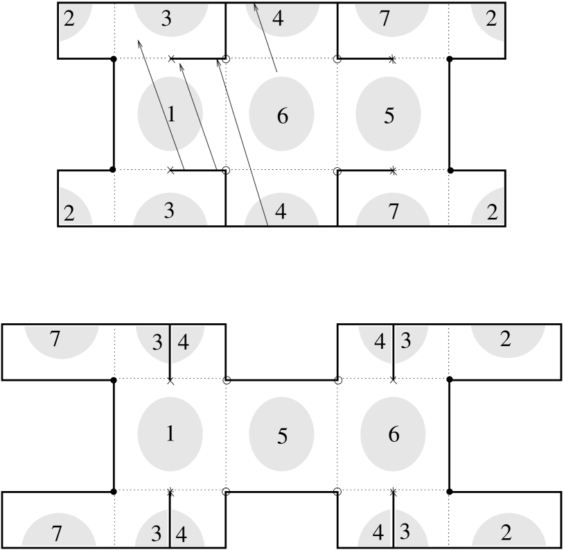
Figure 7: The pair $7_{3}$ of isospectral billiards with a rectangular base shape unfolded to a translation surface (i.e. flat billiard with opposite sides identified).

Opposite sides are identified (e.g. in the first surface, the left edge of tile 1 is identified with the right edge of tile 5). Each surface has four singular points. The symbols $\circ$ and $\bullet$ represent a $6\pi$-angle, while the $\times$ and $\ast$ symbols denote a $8\pi$ angle. An example of a straight line drawn on the first surface is shown on Fig. 7. The eigenvalue problem on these surfaces is equivalent to the problem on the billiards. It is however simpler to handle since the translation surfaces have no boundary. Thus, only the continuity properties of the eigenfunctions have to be checked.

Each translation surface is tiled by seven rectangles. Again, any point on the surface can be specified by its coordinates $({\bf a},i)$. Each tile on the translation surface has six neighboring tiles, attached at its left, upper left, upper right, right, lower right and lower left edge, and numbered from 1 to 6 respectively. For instance tile 1 is surrounded by: tile 5 on its left edge, tile 6 on its right edge, tile 3 on its upper left edge, tile 1 itself on its upper right edge (because of the identification of opposite sides), tile 3 on its lower left edge and tile 1 on its lower right edge. The way the tiles are glued together can be specified by permutation matrices $A^{(\nu)}$, $1\leq\nu\leq 6$, such that $A^{(\nu)}_{ij}=1$ if and only if the edge number $\nu$ of $i$ glues tile $i$ to tile $j$. For instance for the first translation surface, the matrix specifying which tile is on the right of which is

$$A^{(2)}=\left(\begin{array}[]{ccccccc}0&0&0&0&0&1&0\cr 0&0&1&0&0&0&0\cr 0&0&0&0&0&0&1\cr 0&0&0&1&0&0&0\cr 1&0&0&0&0&0&0\cr 0&0&0&0&1&0&0\cr 0&1&0&0&0&0&0\cr\end{array}\right)$$ (6)

(tile 6 is on the right of tile 1, therefore $A^{(1)}_{1,6}=1$, and so on). In a similar way, matrices $B^{(\nu)}$, $1\leq\nu\leq 6$, can be defined for the second translation surface. Now suppose there exists a matrix $T$ such that

$$\forall\nu,\ 1\leq\nu\leq 6,\ A^{(\nu)}T=TB^{(\nu)}.$$ (7)

Then for any given eigenstate $\phi$ of the first translation surface we can construct an eigenstate $\psi$ for the second translation surface, defined by Eq. (4). In order to prove isospectrality we only have to check for continuity properties at each edge. Suppose tiles $i$ and $j$ are neighbors. This means that there exists a $\nu$, $1\leq\nu\leq 6$, such that $A^{(\nu)}_{ij}=1$. To prove the continuity of $\psi$ between tiles $i$ and $j$, we have to show that the quantity

$$\mathcal{C}=\psi({\bf a},i)-\psi({\bf a},j)$$ (8)

is equal to zero for all ${\bf a}$ belonging to the edge between $i$ and $j$. By definition of $\nu$ we have $A^{(\nu)}_{ik}=1$ if and only if $k=j$. Therefore

$$\psi({\bf a},j)=\sum_{k}A^{(\nu)}_{ik}\psi({\bf a},k),$$ (9)

and $\mathcal{C}$ is given by

$$\mathcal{C}=\psi({\bf a},i)-\sum_{k}A^{(\nu)}_{ik}\psi({\bf a},k).$$ (10)

Using Eq. (4), we get

$$\mathcal{C}=\mathcal{N}\sum_{k}T_{ik}\phi({\bf a},k)-\mathcal{N}\sum_{k,k^{\prime}}A^{(\nu)}_{ik}T_{kk^{\prime}}\phi({\bf a},k^{\prime}).$$ (11)

The sum over $k$ on the right-hand side yields a term $(A^{(\nu)}T)_{ik^{\prime}}$. According to the commutation relation (7), it is equal to $(TB^{(\nu)})_{ik^{\prime}}$, which gives

$$\mathcal{C}=\sum_{k}T_{ik}\left(\phi({\bf a},k)-\sum_{k^{\prime}}B^{(\nu)}_{kk^{\prime}}\phi({\bf a},k^{\prime})\right).$$ (12)

Now the continuity of the function $\phi$ ensures that all the terms between parentheses vanish. Thus $\mathcal{C}=0$, and continuity of $\psi$ is proved. Continuity of partial derivatives is proved in the same way.

The proof rests entirely on the fact that we assumed the existence of a transplantation matrix $T$ satisfying the commutation properties (7). It turns out that such a matrix exists. One can check that given the matrix

$$T=\left(\begin{array}[]{ccccccc}1&0&0&1&0&0&1\cr 0&1&0&0&1&0&1\cr 0&0&1&0&0&1&1\cr 1&0&0&0&1&1&0\cr 0&1&0&1&0&1&0\cr 0&0&1&1&1&0&0\cr 1&1&1&0&0&0&0\cr\end{array}\right),$$ (13)

the commutation relations (7) are satisfied for all $\nu$, $1\leq\nu\leq 6$. Thus the proof of isospectrality is completed. We return in section IV on this transplantation proof of isospectrality.

A natural question is to know how one can find a suitable matrix $T$ and permutation matrices $A^{(\nu)}$, $B^{(\nu)}$ verifying all commutation equations (7). Historically these matrices were obtained by the construction of Sunada triples, as will be explained in section VII.3. In fact, it turns out that the matrix $T$ is just the incidence matrix of the graph associated with a certain finite projective space (the Fano plane in our example), as will be explained in detail in section IV.

III Further Examples in Higher Dimensions

Milnor (1964) showed that from two nonisometric lattices of rank $16$ in $\mathbb{R}^{16}$ discovered by Witt (1941), one can construct a pair of flat tori that have the same spectrum of eigenvalues (all relevant terms are defined below).

In this section, we describe a simple criterion for the construction of nonisometric flat tori with the same eigenvalues for the Laplace operator, from certain lattices (which was used by Milnor for the particular case mentioned above), and then we construct, for each integer $n\geq 17$, a pair of lattices of rank $n$ in $\mathbb{R}^{n}$ that match the criterion. Furthermore, we describe results of S. Wolpert and M. Kneser on the moduli space of flat tori. An interesting survey paper focused on the (elementary) construction theory of isospectral manifolds has been given by Brooks (1988).

III.1 Lattices and flat tori

A lattice (that is, a discrete additive subgroup) can be prescribed as $A\mathbb{Z}^{n}$ with $A$ a fixed matrix. For example, set

$$A=\left(\begin{array}[]{cc}1&0\\ 1&1\\ \end{array}\right);$$ (14)

then the lattice $A\mathbb{Z}^{2}$ consists of the points of the form

$$a(1,1)+b(0,1),\ \ a,b\in\mathbb{Z}.$$ (15)

An $n$-dimensional (flat) torus $T$ is $\mathbb{R}^{n}$ factored by a lattice $\mathbf{L}=A\mathbb{Z}^{n}$ with $A\in\mathbf{GL}(n,\mathbb{R})$. The torus is thus determined by identifying points that differ by an element of the lattice.

If we return to the planar example above, the torus topologically is a donut — one may see this by cutting out the parallelogram determined by $(1,1)$ and $(0,1)$, and then gluing opposite sides together.

With $A,B\in\mathbf{GL}(n,\mathbb{R})$ are associated the lattices $A\mathbb{Z}^{n}$ and $B\mathbb{Z}^{n}$. The tori $\mathbb{R}^{n}/A\mathbb{Z}^{n}$ and $\mathbb{R}^{n}/B\mathbb{Z}^{n}$, $B\in\mathbf{GL}(n,\mathbb{R})$, are isometric if and only if $A\mathbb{Z}^{n}$ and $B\mathbb{Z}^{n}$ are isometric by left multiplication by an element of $\mathbf{O}(n,\mathbb{R})$. The matrices $A$ and $B$ are associated with the same lattice if and only if they are equivalent by multiplication on the right by an element of $\mathbf{GL}(n,\mathbb{Z})$. So the tori $\mathbb{R}^{n}/A\mathbb{Z}^{n}$ and $\mathbb{R}^{n}/B\mathbb{Z}^{n}$ are isometric if and only if $A$ and $B$ are equivalent in

$$\mathbf{O}(n,\mathbb{R})\setminus\mathbf{GL}(n,\mathbb{R})/\mathbf{GL}(n,\mathbb{Z}).$$ (16)

Here, $\mathbf{O}(n,\mathbb{R})$ is the orthogonal group in $n$ dimensions.

The metric structure of $\mathbb{R}^{n}$ projects to $T$, and volume$(T)=|\mbox{det}A|$; $T$ carries a Laplace operator

$$\Delta=-\sum_{i}\partial^{2}/\partial x_{i}^{2},$$ (17)

which is just the projection of the Laplacian of $\mathbb{R}^{n}$. The lengths of closed geodesics of $T$ are given by $\parallel a\parallel$ for $a$ arbitrary in $\mathbf{L}$, $\parallel\cdot\parallel$ being the Euclidean norm.

Let $P$ be a symmetric matrix that defines a quadratic form on $\mathbb{R}^{n}$. The spectrum of $P$ is defined to be the sequence (with multiplicities) of values $\gamma=N^{T}PN$ for $N\in\mathbb{Z}^{n}$. The sequence of squares of lengths of closed geodesics of $\mathbb{R}^{n}/A\mathbb{Z}^{n}$ is the spectrum of $A^{T}A=Q$; the sequence of eigenvalues of the Laplacian is the spectrum of $4\pi^{2}(A^{-1})(A^{-1})^{T}=4\pi^{2}Q^{-1}$. The Jacobi inversion formula yields for positive $\tau$,

$$\sum_{N\in\mathbb{Z}^{n}}\mbox{exp}(-4\pi^{2}\tau N^{T}Q^{-1}N)\hskip 56.9055pt$$

$$=\frac{\mbox{volume}(T)}{(4\pi\tau)^{n/2}}\sum_{M\in\mathbb{Z}^{n}}\mbox{exp}(\frac{-1}{4\tau}M^{T}QM).$$ (18)

This equation therefore relates the eigenvalue spectrum of the torus to its length spectrum. We will see in section V.2.3 other examples of this connection between the spectrum of the Laplacian and the length spectrum.

III.2 Construction of examples

If $\mathbf{L}$ is a lattice of $\mathbb{R}^{n}$, $\mathbf{L}^{*}$ denotes its dual lattice, which consists of all $y\in\mathbb{R}^{n}$ for which $\langle x,y\rangle\in\mathbb{Z}$ for all $x\in\mathbf{L}$; here, $\langle\cdot,\cdot\rangle$ is the usual scalar product on $\mathbb{R}^{n}\times\mathbb{R}^{n}$. Clearly, ${(\mathbf{L}^{*})}^{*}=\mathbf{L}$, and two lattices $\mathbf{L}$ and $\mathbf{L}^{\prime}$ are isometric if and only if $\mathbf{L}^{*}$ and ${\mathbf{L}^{\prime}}^{*}$ are.

Recall that two flat tori of the form $\mathbb{R}^{n}/\mathbf{L}_{i}$, $i\in\{1,2\}$, are isometric if and only if the lattices $\mathbf{L}_{1}$ and $\mathbf{L}_{2}$ are isometric. The following theorem gives a criterion for isospectrality of flat tori.

Theorem III.1

Let $\mathbf{L}_{1}$ and $\mathbf{L}_{2}$ be two nonisometric lattices of rank $n$ in $\mathbb{R}^{n}$, $n\geq 2$, and suppose that for each $r>0$ in $\mathbb{R}$, the ball of radius $r$ about the origin contains the same number of points of $\mathbf{L}_{1}$ and $\mathbf{L}_{2}$. Then the flat tori $\mathbb{R}^{n}/\mathbf{L}_{1}^{*}$ and $\mathbb{R}^{n}/\mathbf{L}_{2}^{*}$ are nonisometric while having the same spectrum for the Laplace operator.

Proof. Suppose $x\neq\mathbf{0}$ is an element of $\mathbf{L}_{1}$ of length $\alpha$. Then there is an $\alpha^{\prime}<\alpha$ such that the ball of radius $\alpha^{\prime}$ centered at $\mathbf{0}$ contains all elements of $\mathbf{L}_{1}$ with length strictly smaller than $\alpha$ (since $\mathbf{L}_{1}$ is discrete). For any $\alpha^{\prime}\leq\alpha^{\prime\prime}<\alpha$, the ball of radius $\alpha^{\prime\prime}$ centered at $\mathbf{0}$ contains that same number of elements. This ball contains as many elements of $\mathbf{L}_{2}$ as of $\mathbf{L}_{1}$, and since the ball centered at $\mathbf{0}$ with radius $\alpha$ contains strictly more elements of $\mathbf{L}_{1}$, it follows easily that $\mathbf{L}_{2}$ also contains vectors of length $\alpha$.

Each element $z\in\mathbf{L}_{i}$, $i\in\{1,2\}$, determines an eigenfunction $f(x)=e^{2\pi\langle x,z\rangle i}$ for the Laplace operator on $\mathbb{R}^{n}/\mathbf{L}_{i}^{*}$, with corresponding eigenvalue $\lambda=(2\pi)^{2}\langle z,z\rangle$, so the number of eigenvalues less than or equal to $(2\pi r)^{2}$ is equal to the number of points of $\mathbf{L}_{i}$ contained in the ball centered at $\mathbf{0}$ with radius $r$.

We conclude that $\mathbb{R}^{n}/\mathbf{L}_{1}^{*}$ and $\mathbb{R}^{n}/\mathbf{L}_{2}^{*}$ have the same spectrum of eigenvalues, while not being isometric. $\blacksquare$

Milnor’s Construction. By using the Witt nonisometric lattices in $\mathbb{R}^{16}$ Witt (1941), Milnor (1964) essentially used the aforementioned criterion to construct the first example of nonisometric isospectral flat tori.

Starting from these two nonisometric lattices $\mathbf{L}_{1}^{16}$ and $\mathbf{L}_{2}^{16}$ of rank $16$ in $\mathbb{R}^{16}$ as described in Witt (1941), one can in fact construct examples of isospectral flat tori in $\mathbb{R}^{n}$ for all $n$, $n\geq 16$, as follows. The lattices $\mathbf{L}_{1}^{16}$ and $\mathbf{L}_{2}^{16}$ satisfy the condition of Theorem III.1 (Witt, 1941, p. 324). Now embed $\mathbb{R}^{16}$ in $\mathbb{R}^{17}$ in the canonical way. Denote the coordinate axes of the latter by $X_{1},X_{2},\ldots,X_{17}$, such that $\langle X_{1},X_{2},\ldots,X_{16}\rangle=\mathbb{R}^{16}$. Suppose $\ell\neq\mathbf{0}$ is a vector on the $X_{17}$-axis which has length strictly smaller than any non-zero vector of $\mathbf{L}_{1}$ (and $\mathbf{L}_{2}$). Define two new lattices $\mathbf{L}_{i}^{17}$ (of rank $17$) generated by $\mathbf{L}_{i}^{16}$ and $\ell$, $i=1,2$. Since $X_{17}\perp\mathbb{R}^{16}$, it follows easily that for any $r>0$, the ball centered at the origin with radius $r$ contains the same number of elements of $\mathbf{L}_{1}^{17}$ as of $\mathbf{L}_{2}^{17}$. One observes that these lattices are nonisometric. Thus, by Theorem III.1, we obtain two nonisometric flat tori $\mathbb{R}^{17}/{\mathbf{L}_{i}^{17}}^{*}$, $i=1,2$, which have the same spectrum of eigenvalues for the Laplace operator.

Inductively, we can now define, in a similar way, the nonisometric lattices $\mathbf{L}_{1}^{n}$ and $\mathbf{L}_{2}^{n}$ of rank $n$, $n\geq 17$, satisfying the condition of Theorem III.1, and thus leading to nonisometric flat tori $\mathbb{R}^{n}/{\mathbf{L}_{i}^{n}}^{*}$, $i=1,2$, which have the same spectrum of eigenvalues for the Laplace operator.

III.3 The four-parameter family of Conway and Sloane

Let $\Lambda$ be a positive-definite lattice. The theta function of $\Lambda$ is:

$$\Theta_{\Lambda}(\tau)=\sum_{x\in\Lambda}e^{i\pi\tau\parallel x\parallel^{2}}=\sum_{x\in\Lambda}q^{\parallel x\parallel^{2}}=\sum_{m=0}^{\infty}N_{m}q^{m},$$ (19)

where $\mathrm{Im}(\tau)>0$, and $N_{m}$ is the number of vectors $x\in\Lambda$ of norm $m$. $\Theta_{\Lambda}$ can be thought of as a formal power series in the indeterminate $q$, although sometimes one takes $q=e^{i\pi\tau}$ for further investigation, with $\tau$ a complex variable. In that case, $\Theta_{\Lambda}(\tau)$ is a holomorphic function of $\tau$ for $\mathrm{Im}(\tau)\geq 0$.

Conway and Sloane (1992) construct a four-parameter family of pairs of four-dimensional lattices that are isospectral (equivalently, that have the same theta series (19)). In a similar way as before, such lattice pairs yield isospectral flat tori. The main construction of Conway and Sloane (1992) is given by the next result.

Theorem III.2 (Conway and Sloane, 1992)

Let $e_{\infty}$, $e_{0}$, $e_{1}$, $e_{2}$ be orthogonal vectors satisfying

$$e_{\infty}\cdot e_{\infty}=a/12,\ \ e_{0}\cdot e_{0}=b/12,\ \ e_{1}\cdot e_{1}=c/12,\ \ e_{2}\cdot e_{2}=d/12,$$

where $a,b,c,d>0$, and let $[w,x,y,z]$ denote the vector $we_{\infty}+xe_{0}+ye_{1}+ze_{2}$. Let $v_{\infty}^{\pm}=[\pm 3,-1,-1,-1],v_{0}^{\pm}=[1,\pm 3,1,-1],v_{1}^{\pm}=[1,-1,\pm 3,1],v_{2}^{\pm}=[1,1,-1,\pm 3]$. Then the lattices $\mathbf{L}^{+}(a,b,c,d)$ spanned by $v_{\infty}^{+},v_{0}^{+},v_{1}^{+},v_{2}^{+}$ and $\mathbf{L}^{-}(a,b,c,d)$ spanned by $v_{\infty}^{-},v_{0}^{-},v_{1}^{-},v_{2}^{-}$ are isospectral.

Some small values of $a,b,c,d$ give examples which were first found by Schiemann (1990). Substituting $(a,b,c,d)=(7,13,19,49)$, one obtains the pair of Earnest and Nipp (1991).

III.4 The eigenvalue spectrum as moduli for flat tori

We now discuss some interesting results on the eigenvalue spectrum for flat tori. We already saw that there exist nonisometric isospectral flat tori. A natural question is now how such tori are distributed.

The following theorem gives an insight into this question by considering the case of a continuous family of isospectral flat tori.

Theorem III.3 (Wolpert (1978))

Let $T_{s}$ be a continuous family of isospectral tori defined for $s\in[0,1]$. Then the tori $T_{s}$, $s\in[0,1]$, are isometric.

An interesting result by M. Kneser is the following (see Wolpert (1978) for a proof). It states that, given an eigenvalue spectrum of some torus, only a finite number of nonisometric tori can be isospectral to it.

Theorem III.4 (M. Kneser)

The total number of nonisometric tori with a given eigenvalue spectrum is finite.

The following result is rather technical. Its main message is that given two tori $\mathbb{R}^{n}/A\mathbb{Z}^{n}$ and $\mathbb{R}^{n}/B\mathbb{Z}^{n}$ with the same eigenvalue spectrum, then either these two tori are isometric, or the quadratic forms $(A^{T}A)$ and $(B^{T}B)$ lie on a certain subvariety in the space of positive definite quadratic forms. A more precise statement is as follows. Denote the space of positive definite symmetric $n\times n$-matrices by $\wp(n,\mathbb{R})$, and observe that the map

$$A\in\mathbf{GL}(n,\mathbb{R})\mapsto A^{T}A\in\wp(n,\mathbb{R})$$ (20)

determines a bijection from $\mathbf{O}(n,\mathbb{R})\setminus\mathbf{GL}(n,\mathbb{R})$ to $\wp(n,\mathbb{R})$. Then the following theorem holds.

Theorem III.5 (Wolpert (1978))

There is a properly discontinuous group $G_{n}$ acting on $\wp(n,\mathbb{R})$ containing the transformation group induced by the $\mathbf{GL}(n,\mathbb{Z})$ action

$$S\mapsto A[\mathcal{Z}],$$ (21)

where $S\in\wp(n,\mathbb{R})$ and $\mathcal{Z}\in\mathbf{GL}(n,\mathbb{Z})$. Given $P,S\in\wp(n,\mathbb{R})$ with the same spectrum, either $g(P)=S$ for some $g\in G_{n}$, or $P,S\in\mathfrak{V}_{n}$, where the latter is a subvariety of $\wp(n,\mathbb{R})$. Moreover,

• $\mathfrak{V}_{n}=\{Q\in\wp(n,\mathbb{R})\parallel$ spec(Q) $=$ spec(R), $R\in\wp(n,\mathbb{R})$ with $R\neq g(Q)$ for all $g\in G_{n}\}$, and

• $\mathfrak{V}_{n}$ is the intersection of $\wp(n,\mathbb{R})$ and a countable union of subspaces of $\mathbb{R}^{m}$ for some $m$.

In this section we have seen that is essentially “easy” to construct (nonisometric) isospectral flat tori. The Milnor example was exhibited in 1964. But it has taken about 30 years to find counterexamples to Kac’s question in the real plane …

IV Transplantation

The aim of this section is to describe the idea of transplantation in a more mathematical way than in section II. This concept was presumably first introduced by Bérard (1992, 1993). There is in fact a deep connection between transplantation theory and the mathematical field of finite geometries. First we review some elementary facts about finite geometries. Application of these tools to transplantation theory sheds light on the reasons for the existence of isospectrality.

IV.1 Tiling

IV.1.1 Graphs and billiards by tiling

In this section, we follow Okada and Shudo (2001).

Tiling. All known isospectral billiards can be obtained by unfolding polygonal-shaped tiles. As the unfolding is done along only three sides of the polygon we can essentially consider triangles. We call such examples isospectral Euclidean TI-domains. The known ones are listed in Appendix A. The way the tiles are unfolded can be specified by three permutation $d\times d$-matrices $M^{(\mu)}$, $1\leq\mu\leq 3$ and $d\in\mathbb{N}$, associated with the three sides of the triangle and defined in the following way: $M^{(\mu)}_{ij}=1$ if tiles $i$ and $j$ are glued by their side $\mu$; $M^{(\mu)}_{ii}=1$ if the side $\mu$ of tile $i$ is the boundary of the billiard, and $0$ otherwise. The number of tiles is, of course, $d$. Call the matrices $M^{(\mu)}$ “adjacency matrices”.

One can sum up the action of the $M^{(\mu)}$ in a graph with colored edges: each copy of the base tile is associated with a vertex, and vertices $i$ and $j$, $i\neq j$, are joined by an edge of color $\mu$ if and only if $M^{(\mu)}_{ij}=1$. In the same way, in the second member of the pair, the tiles are unfolded according to permutation matrices $N^{(\mu)}$, $1\leq\mu\leq 3$. We call such a colored graph an involution graph for reasons to be explained later in this section. An example of such graphs is given in Fig. 4. If $D$ is a Euclidean TI-domain with base tile a triangle, and $\mathfrak{M}=\{M^{(\mu)}\parallel\mu\in\{1,2,3\}\}$ is the set of associated permutation matrices (or, equivalently, the associated coloring), denote by $\Gamma(D,\mathfrak{M})$ the corresponding involution graph.

The following proposition is easy but rather useful Thas (2007b).

Proposition IV.1

Let $D$ be a Euclidean TI-domain with base tile a triangle, and let $\mathfrak{M}=\{M^{(\mu)}\parallel\mu\in\{1,2,3\}\}$ be the set of associated permutation matrices. Then the matrix

$$\Delta_{ij}=\sum_{\mu=1}^{3}\left(M^{(\mu)}_{ij}-M^{(\mu)}_{ii}\delta_{ij}\right),$$ (22)

where $\delta_{ij}$ is the Kronecker symbol, is the adjacency matrix of $\Gamma(D,\mathfrak{M})$.$\blacksquare$

Transplantability. Two billiards are said to be transplantable if there exists an invertible matrix $T$ — the transplantation matrix — such that

$$TM^{(\mu)}=N^{(\mu)}T\ \ \mbox{for all}\ \ \mu.$$ (23)

If the matrix $T$ is a permutation matrix, the two domains would just have the same shape. One can show that transplantability implies isospectrality, as seen in section II.

We now discuss an example exhibited by Buser et al. (1994), and first found by Gordon et al. (1992a).

IV.1.2 The example of Gordon et al.

Buser (1988) constructed a pairs of isospectral flat surfaces $\mathfrak{M}_{1}$ and $\mathfrak{M}_{2}$ as covers of a certain surface $\mathfrak{M}_{0}$, using a pair of almost conjugate subgroups of $\mathbf{SL}(3,2)$. Gordon et al. (1992a) similarly constructed orbifolds $O_{1}$ and $O_{2}$, respectively being the quotient by an involutive isometry of $\mathfrak{M}_{1}$ and $\mathfrak{M}_{2}$. $O_{1}$ and $O_{2}$ have a common orbifold cover — it is the quotient by an involutive isometry of the common cover of $\mathfrak{M}_{1}$ and $\mathfrak{M}_{2}$. The Neumann orbifold spectrum of $O_{i}$ is precisely the Neumann spectrum of the underlying manifold $\mathfrak{M}(O_{i})$, and these latter underlying spaces are simply connected real plane domains. Furthermore, Dirichlet isospectrality of $\mathfrak{M}(O_{1})$ and $\mathfrak{M}(O_{2})$ is obtained by exploiting the Dirichlet isospectrality of $\mathfrak{M}_{1}$ and $\mathfrak{M}_{2}$.

We now analyze this pair of isospectral but non-congruent Euclidean domains. We follow the very transparent approach of Buser et al. (1994) to show isospectrality. As the reader will notice, this will in fact be an easy approach to (and example of) transplantability.

Figure 8: Two isospectral billiards with a triangular base shape on seven tiles.

Setting. Let $f$ be an eigenfunction of the Laplacian with eigenvalue $\lambda\in\mathbb{R}$ for the Dirichlet problem corresponding to the left-hand billiard in Fig. 8. Let $f_{0},f_{1},\ldots,f_{6}$ denote the functions obtained by restriction of $f$ to each of the seven tiles of the left-hand billiard, as indicated on the left in Fig. 8. For the sake of convenience, we write $\mathbf{i}$ for $f_{i}$.

The Dirichlet boundary condition is that $f$ must vanish on each boundary segment. This is equivalent to the assertion that $f$ goes into $-f$ if continued as a smooth eigenfunction across any boundary segment; in fact, it goes into $f\circ\sigma$ where $\sigma$ is the reflection on the boundary segment.

On the right in Fig. 8, we show how to obtain from $f$ another eigenfunction of eigenvalue $\lambda$ for the right-hand domain. We define the function $\mathbf{1}+\mathbf{2}+\mathbf{4}$ which is actually the function

$$f_{1}\circ\tau_{1}+f_{2}\circ\tau_{2}+f_{4}\circ\tau_{4},$$ (24)

where for $k=1,2,4$, $\tau_{k}$ is the isometry from the central triangle of the right-hand billiard to the triangle labeled $k$ on the left-hand one. Now we see from the left-hand side that the functions $\mathbf{1},\mathbf{2},\mathbf{4}$ continue smoothly across dotted lines into copies of the functions $\mathbf{0},\mathbf{5},-\mathbf{4}$ respectively, so that their sum continues into $\mathbf{0}+\mathbf{5}-\mathbf{4}$ as shown. Similarly way one observes that this continues across a solid line to $\mathbf{4}-\mathbf{5}-\mathbf{0}$ (its negative), and across a dashed line to $\mathbf{2}-\mathbf{5}-\mathbf{3}$, which continues across either a solid or dotted line to its own negative. These assertions, together with the similar ones obtained by cyclic permutation of the arms of the billiards, suffice to show that the transplanted function is an eigenfunction of the eigenvalue $\lambda$ that vanishes along each boundary segment of the right-hand domain.

We have defined a linear map which for each $\lambda$ transforms the $\lambda$-eigenspace for the left-hand billiard into the $\lambda$-eigenspace for the right-hand one. This is a non-singular map (the corresponding matrix is non-singular), and so the dimension of the eigenspace on the right-hand side is larger than or equal to the dimension on the left-hand side. By symmetry, it follows that the dimensions are equal. Since $\lambda$ was arbitrary, the two billiards are Dirichlet isospectral.

IV.1.3 The other known examples

A similar technique as in the previous section allowed Buser et al. (1994) to show that the series of billiard pairs they produced are indeed isospectral. All these pairs are listed in Appendix A; they were first found by searching for suitable Sunada triples, and then verified to be isospectral (in the plane) by the transplantation method (see also Okada and Shudo (2001) for a further discussion about the subject of this section).

IV.1.4 Euclidean TI-domains and their involution graphs

To conclude this section, we address a related problem, namely isospectrality of the involution graphs associated with the isospectral billiards. We say that two (undirected) graphs are isospectral if their adjacency matrices have the same multiset of eigenvalues. Note that this definition of graph isospectrality is different from the definition introduced in e.g. Gutkin and Smilansky (2001), where the spectrum of a metric graph is defined as the spectrum of the Laplacian on the graph whose edges are assigned a given length.

The following question was posed by Thas (2007b): Let $(D_{1},D_{2})$ be a pair of nonisometric isospectral Euclidean TI-domains, and let $\Gamma(D_{1})=\Gamma(D_{1},\{M^{(\mu)}\parallel\mu\in\{1,2,3\}\})$ and $\Gamma(D_{2})=\Gamma(D_{2},\{N^{(\mu)}\parallel\mu\in\{1,2,3\}\})$ be the corresponding involution graphs. Are $\Gamma(D_{1})$ and $\Gamma(D_{2})$ isospectral? Note that one does not require the domains to be transplantable. (The term “cospectrality” is also sometimes used in graph theory, instead of “isospectrality”.)

We now show that the answer is “yes” when the domains are transplantable. The proof is taken from Thas (2007b).

Theorem IV.2

Let $(D_{1},D_{2})$ be a pair of nonisometric isospectral Euclidean TI-domains, and let $\Gamma(D_{1})=\Gamma(D_{1},\{M^{(\mu)}\parallel\mu\in\{1,2,3\}\})$ and $\Gamma(D_{2})=\Gamma(D_{2},\{N^{(\mu)}\parallel\mu\in\{1,2,3\}\})$ be the corresponding involution graphs. Then $\Gamma(D_{1})$ and $\Gamma(D_{2})$ are isospectral.

Proof. Define, for $\mu=1,2,3$, $M^{(\mu)}_{*}$ as the matrix which has the same entries as $M^{(\mu)}$, except on the diagonal, where it has only zeros. Define matrices $N^{(\mu)}_{*}$ analogously. Suppose that $TM^{(\mu)}T^{-1}=N^{(\mu)}$ for all $\mu$. Note the following properties:

• $M^{(\mu)}_{*}$ and $N^{(\mu)}_{*}$, $\mu=1,2,3$, are symmetric $(0,1)$-matrices, with at most one $1$ entry on each row;

• $[M^{(\mu)}_{*}]^{m}=M^{(\mu)}_{*}$ if the natural number $m$ is odd and $[M^{(\mu)}_{*}]^{m}=\mathbb{I}_{M}^{(\mu)}$, where $[\mathbb{I}_{M}^{(\mu)}]_{ii}=1$ if there is a $1$ on the $i$-th row of $M_{*}^{(\mu)}$, and $0$ otherwise, if $m$ is even, $\mu=1,2,3$, and similar properties hold for the $N^{(\mu)}_{*}$;

• $\mbox{Tr}(M^{(i)}_{*}M^{(j)}_{*})=\mbox{Tr}(M^{(j)}_{*}M^{(i)}_{*})=0$ for $i\neq j$ and $\mbox{Tr}(N^{(i)}_{*}N^{(j)}_{*})=\mbox{Tr}(N^{(j)}_{*}N^{(i)}_{*})=0$ for $i\neq j$;

• $\mbox{Tr}(M^{(i)}_{*}M^{(j)}_{*}M^{(k)}_{*})$ and $\mbox{Tr}(N^{(i)}_{*}N^{(j)}_{*}N^{(k)}_{*})$ are independent of the permutation $(ijk)$ of $(123)$ (this is because the individual matrices are symmetric);

• the value of all traces in the previous property is $0$ (note that, if $\{i,j,k\}=\{1,2,3\}$, such a trace equals $0$ since the existence of a nonzero diagonal entry of $M^{(i)}_{*}M^{(j)}_{*}M^{(k)}_{*}$, respectively $N^{(i)}_{*}N^{(j)}_{*}N^{(k)}_{*}$, implies $\Gamma(D_{1})$, respectively $\Gamma(D_{2})$, to have closed circuits of length $3$).
  

From Proposition IV.1 it follows that $A=\sum_{\mu=1}^{3}M^{(\mu)}_{*}$ is the adjacency matrix of $\Gamma(D_{1})$, and $B=\sum_{\mu=1}^{3}N^{(\mu)}_{*}$, the adjacency matrix of $\Gamma(D_{2})$.

Consider a natural number $n\in\mathbb{N}_{0}$. Then, with the previous properties in mind, it follows that

$$\mbox{Tr}(A^{n})=\mbox{Tr}(B^{n}).$$ (25)

Thus by the following lemma (cf. (van Dam and Haemers, 2003, Lemma 1)) the adjacency matrices of $\Gamma(D_{1})$ and $\Gamma(D_{2})$ have the same spectrum.

Lemma IV.3

Two $k\times k$-matrices $K$ and $K^{\prime}$ are isospectral if and only if Tr$(K^{l})=$ Tr$({K^{\prime}}^{l})$ for $l=1,2,\ldots,k$.

$\blacksquare$
In section VIII we will see that other graph theoretical problems turn up in Kac theory.

IV.2 Some projective geometry

There is a fascinating relation between the structure of isospectral billiards and the geometry of vector spaces over finite fields. In section II we constructed pairs of isospectral billiards using unfolding rules. These unfolding rules can be encoded into graphs, like the ones in Fig. 4. Thus the structure of a pair of isospectral billiards is entirely encoded into a pair of graphs that have certain specific properties. The graphs of Fig. 4 are ”colored” according to a certain set of permutations. It turns out that the group generated by these permutations is precisely the automorphism group of a projective space over a finite field, the so-called Fano plane. The Fano plane has many beautiful properties and appears in various places, such as combinatorial problems or the multiplication table of the octonions. A representation of this finite projective plane is given in Fig. 9. Here we will see that the adjacency matrix of the graph representing the Fano plane is nothing but the transplantation matrix between the two isospectral billiards of Fig. 4.

In order to understand this deep connection, basic notions of finite geometries and design theory are required. In this section we provide the necessary tools. More details about the notions considered here can be found in Hirschfeld (1998). Note that some remarks about isospectrality, projective geometry and groups are made in Vorobets and Stepin (1998), however the results there are not fully mathematically rigorous.

IV.2.1 Finite projective geometry

Let $\mathbb{F}_{q}$ be the finite field with $q$ elements, $q$ a prime power, and denote by $V(n,q)$ the $n$-dimensional vector space over $\mathbb{F}_{q}$, $n$ a nonzero natural number. Define the $(n-1)$-dimensional projective geometry $\mathbf{PG}(n-1,q)$ over $\mathbb{F}_{q}$ as the set of all subspaces of $V(n,q)$. Note that $\mathbf{PG}(n-1,q)$ is often called the “Desarguesian” or “classical” projective space. The projective space $\mathbf{PG}(-1,q)$ is the empty set, and has dimension $-1$.

Points in $\mathbf{PG}(n,q)$ correspond to one-dimensional subspaces of $V(n,q)$, lines in $\mathbf{PG}(n,q)$ correspond to two-dimensional subspaces of $V(n,q)$, and so on. Any $d$-dimensional subspace of $\mathbf{PG}(n,q)$ contains $(q^{d+1}-1)/(q-1)$ points. In particular, $\mathbf{PG}(n,q)$ itself has $(q^{n+1}-1)/(q-1)$ points. It also has $(q^{n+1}-1)/(q-1)$ hyperplanes (i.e. $(n-1)$-dimensional subspaces).

Example. The Fano plane $\mathbf{PG}(2,2)$ shown in Fig. 9 has seven points and seven hyperplanes or lines (one of which is represented as a circle in Fig. 9). Any line contains three points (we say that three points are “incident” with each line) and any point belongs to three lines (we say that three lines are “incident” with each point). The use of the word ‘’incident” in both cases enhances the symmetry between points and lines in this geometry. It is precisely this geometry that lies at the root of isospectrality.

Figure 9: The Fano plane.

IV.2.2 Automorphism groups

The automorphism groups of finite projective spaces play a key role in isospectrality as the generators of these groups allow us to construct the graphs that encode the unfolding rules for the billiard construction. We now define these groups and mention some of their properties. For group theoretical notions not explained here, we refer to the beginning of section VII.

An automorphism or collineation of a finite projective space is a bijection of the points that preserves the type of each subspace (i.e. lines are mapped to lines, and more generally $d$-dimensional spaces to $d$-dimensional spaces) and preserves incidence properties (i.e. intersecting lines are transformed into intersecting lines, etc…). It can be shown that any automorphism of a $\mathbf{PG}(n,q)$, $n\geq 3$, necessarily has the following form:

$$\theta:\mathbf{x}^{T}\mapsto A(\mathbf{x}^{\sigma})^{T},$$ (26)

where $A\in\mathbf{GL}(n+1,q)$, $\sigma$ is a field automorphism of $\mathbb{F}_{q}$, the homogeneous coordinate $\mathbf{x}=(x_{0},x_{1},\ldots,x_{n})$ represents a point of the space (which is determined up to a scalar), and $\mathbf{x}^{\sigma}=(x_{0}^{\sigma},x_{1}^{\sigma},\ldots,x_{n}^{\sigma})$ (recall that $x_{i}^{\sigma}$ is the image of $x_{i}$ under $\sigma$).

The set of automorphisms of a projective space naturally forms a group, and in case of $\mathbf{PG}(n,q)$, $n\geq 3$, this group is denoted by $\mathbf{P\Gamma L}(n+1,q)$. The normal subgroup of $\mathbf{P\Gamma L}(n+1,q)$ which consists of all automorphisms for which the companion field automorphism $\sigma$ is the identity, is the projective general linear group, and denoted by $\mathbf{PGL}(n+1,q)$. So $\mathbf{PGL}(n+1,q)=\mathbf{GL}(n+1,q)/Z(\mathbf{GL}(n+1,q))$, where $Z(\mathbf{GL}(n+1,q))$ is the central subgroup of all scalar matrices of $\mathbf{GL}(n+1,q)$. Similarly one defines $\mathbf{PSL}(n+1,q)=\mathbf{SL}(n+1,q)/Z(\mathbf{SL}(n+1,q))$, where $Z(\mathbf{SL}(n+1,q))$ is the central subgroup of all scalar matrices of $\mathbf{SL}(n+1,q)$ with unit determinant. Recall that $\mathbf{SL}(n+1,q)$ consists of the elements of $\mathbf{GL}(n+1,q)$ with unit determinant.

An elation of $\mathbf{PG}(n,q)$ is an automorphism of which the fixed points structure precisely is a hyperplane, or the space itself. A homology either is the identity, or it is an automorphism that fixes a hyperplane pointwise, and one further point not contained in that hyperplane.

IV.2.3 Involutions in finite projective space

Let $\mathbf{PG}(n,q)$, $n\in\mathbb{N}\cup\{-1\}$, be the $n$-dimensional projective space over the finite field $\mathbb{F}_{q}$ with $q$ elements, so that $q$ is a prime power; we have $|\mathbf{PG}(n,q)|=\frac{q^{n+1}-1}{q-1}$. (Note again that $\mathbf{PG}(-1,q)$ is the empty space.)

We discuss the different types of involutions that can occur in the automorphism group of a finite projective space Segre (1961).

• Baer Involutions. A Baer involution is an involution that is not contained in the linear automorphism group of the space so that $q$ is a square, and it fixes an $n$-dimensional subspace over $\mathbb{F}_{\sqrt{q}}$ pointwise.

• Linear Involutions in Even Characteristic. If $q$ is even, and $\theta$ is an involution that is not of Baer type, $\theta$ must fix an $m$-dimensional subspace of $\mathbf{PG}(n,q)$ pointwise, with $1\leq m\leq n\leq 2m+1$. In fact, to avoid trivialities, one assumes that $m\leq n-1$.

• Linear Involutions in Odd Characteristic. If $\theta$ is a linear involution of $\mathbf{PG}(n,q)$, $q$ odd, the set of fixed points is the union of two disjoint complementary subspaces. Denote these by $\mathbf{PG}(k,q)$ and $\mathbf{PG}(n-k-1,q)$, $k\geq n-k-1>-1$.

We are now ready to explore a connection between Incidence Geometry and Kac Theory.

IV.3 Projective isospectral data

IV.3.1 Transplantation matrices, projective spaces and isospectral data

Suppose one wants to construct a pair of isospectral billiards, starting from a planar polygonal base shape. The idea described in Giraud (2005a) is to start from the transplantation matrix $T$, and choose it in such a way that the existence of commutation relations

$$TM^{(\mu)}=N^{(\mu)}T$$ (27)

for some permutation matrices $M^{(\mu)},N^{(\mu)}$ will be known a priori. This is the case if $T$ is taken to be the incidence matrix of a finite projective space; the matrices $M^{(\mu)}$ and $N^{(\mu)}$ are then permutations of the points and the hyperplanes of the finite projective space.

An $(N,k,\lambda)-$symmetric balanced incomplete block design (SBIBD) is a rank $2$ incidence geometry, defined on a set of $N$ points, each belonging to $N$ subsets (called blocks) such that each block is incident with $k$ points, any two distinct points are contained in exactly $\lambda$ blocks, and each point is incident with $k$ different blocks.

Example. The points and hyperplanes of an $n$-dimensional projective space $\mathbf{PG}(n,q)$ defined over $\mathbb{F}_{q}$ is an $(N,k,\lambda)$-SBIBD with $N=(q^{n+1}-1)/(q-1)$, $k=(q^{n}-1)/(q-1)$ and $\lambda=(q^{n-1}-1)/(q-1)$.
So the Fano plane is a $(7,3,1)-$SBIBD.

Let $\Gamma$ be an $(N,k,\lambda)$-SBIBD. The points and the blocks can be labeled from $0$ to $N-1$. One can define an $N\times N$-incidence matrix $T$ describing to which block each point belongs. The entries $T_{ij}$ of the matrix are $T_{ij}=1$ if the point $j$ belongs to the block $i$, and $0$ otherwise. It is easy to see that the matrix $T$ verifies the relation

$$TT^{T}=\lambda\mathbb{J}+(N-k)\lambda/(k-1)\mathbb{I},$$ (28)

where $\mathbb{J}$ is the $N\times N$-matrix with all entries equal to $1$ and $\mathbb{I}$ the $N\times N$ identity matrix. In particular, the incidence matrix of $\mathbf{PG}(n,q)$ verifies

$$TT^{T}=\lambda\mathbb{J}+(k-\lambda)\mathbb{I}$$ (29)

with $k$ and $\lambda$ as given above.

Any permutation $\sigma$ of the points of a finite projective space can be written as a $d\times d$ permutation matrix $M$ defined by $M_{i\sigma(i)}=1$ and the other entries equal to zero. Here $d$ is the number of points. If $M$ is a permutation matrix associated with an automorphism of the space, then there exists a permutation matrix $N$ such that

$$TM=NT.$$ (30)

In other words, (30) means that permuting the columns of $T$ (which correspond to the hyperplanes of the space) under $M$ is in some sense equivalent to permuting the rows of $T$ (corresponding to the points of the space) under $N$. The reason that this occurs is the concept of “duality”; in a finite projective space the points and hyperplanes play the same role.

Consider a finite projective space $\pi=\mathbf{PG}(n,q)$ with incidence matrix $T$. With each hyperplane in $\pi$ we associate a tile in the first billiard, and to each point in $\pi$ we associate a tile in the second billiard. If we choose permutations $M^{(\mu)}$ in $\mathbf{P\Gamma L}(n+1,q)$, then the commutation relation (30) will ensure that there exist permutations $N^{(\mu)}$ verifying

$$TM^{(\mu)}=N^{(\mu)}T.$$ (31)

Since these commutation relations imply transplantability, they also imply isospectrality of the billiards constructed from the graphs corresponding to $M^{(\mu)}$ and $N^{(\mu)}$.

Constraints. If the base tile has $r$ sides, we need to choose $r$ elements $M^{(\mu)}$, $1\leq\mu\leq r$, in $\mathbf{P\Gamma L}(n+1,q)$ in such a way that (at least) the following remarks are taken into account.

• Since $M^{(\mu)}$ represents the reflection of a tile with respect to one of its sides, it has to be an involution.

• In order that the billiards be connected, no point should be left out by the matrices $M^{(\mu)}$ — in other words, the graph associated to the matrices $M^{(\mu)}$ should be connected.

• If we want the base tile to be of “any” shape, there should be no closed circuit in the graph (in other words, it should be a finite tree).

Assume one is looking for a pair of isospectral billiards with $d=(q^{3}-1)/(q-1)$ copies of a base tile having the shape of an $r$-gon, $r\geq 3$. We need to search for $r$ involutions such that the associated graph is connected and does not admit a closed circuit. Such a graph connects $d$ vertices and hence requires $d-1$ edges. For involutions with $s$ fixed points, there are $(d-s)/2$ independent transpositions in its cycle decomposition, and each transposition is represented by an edge in the graph. As a consequence, $q$, $r$ and $s$ have to satisfy the following condition:

$$r(q^{2}+q+1-s)/2=q^{2}+q.$$ (32)

More generally, we define “projective isospectral data” as triples $(\mathbf{P},\{\theta^{(i)}\},r)$, where $\mathbf{P}$ is a finite projective space of dimension at least $2$, and $\{\theta^{(i)}\}$ a set of $r$ nontrivial involutions of $\mathbf{P}$, satisfying the following equation

$$r(|\mathbf{P}|-\mbox{Fix}(\theta))=2(|\mathbf{P}|-1),$$ (33)

for some natural number $r\geq 3$. Here Fix$(\theta)$ = Fix$(\theta^{(i)})$ is a constant number of fixed points of $\mathbf{P}$ under each $\theta^{(i)}$, and $|\mathbf{P}|$ is the number of points of $\mathbf{P}$.

One can now generate all possible pairs of isospectral billiards whose transplantation matrix is the incidence matrix of a $\mathbf{PG}(2,q)$, with $r$ and $q$ restricted by the previous analysis.

Using the classification of involutions for dimension $2$, we examine the various cases.

Let $q$ be even and not a square. Then any involution is an elation and therefore has $q+1$ fixed points. Therefore, $q$ and $r$ are constrained by the relation

$$rq^{2}/2=q^{2}+q.$$ (34)

The only integer solution with $r\geq 3$ and $q\geq 2$ is $(r=3,q=2)$. These isospectral billiards correspond to the Fano plane $\mathbf{PG}(2,2)$ and will be made of $d=7$ copies of a base triangle.

Let $q$ be odd and not a square. Then any involution is a homology and therefore has $q+2$ fixed points. Therefore, $q$ and $r$ are constrained by the relation

$$r(q^{2}-1)/2=q^{2}+q.$$ (35)

The only integer solution with $r\geq 3$ and $q\geq 2$ is $(r=3,q=3)$. These isospectral billiards correspond to $\mathbf{PG}(2,3)$ and will be made of $d=13$ copies of a base triangle.

Let $q=p^{2}$ be a square. Then any involution fixes all points in a Baer subplane $\mathbf{PG}(2,p)$ and therefore has $p^{2}+p+1$ fixed points. Therefore, $p$ and $r$ are constrained by the relation

$$r(p^{4}-p)/2=p^{4}+p^{2}.$$ (36)

There is no integer solution with $r\geq 3$ and $q\geq 2$.

Closed circuits. One could also look for isospectral billiards with closed circuits: this will require the base tile to have a shape such that the closed circuit does not make the copies of the tiles come on top of each other when unfolded. If we allow just one closed circuit in the graph describing the isospectral billiards, then there are $d$ edges in the graph instead of $d-1$ and the equation for $p$ and $r$ becomes

$$r(p^{4}-p)/2=p^{4}+p^{2}+1,$$ (37)

which has the only integer solution $(r=3,p=2)$. These isospectral billiards correspond to $\mathbf{PG}(2,4)$ and will be made of $d=21$ copies of a base triangle.

To summarize, we have the following:

• The Fano plane $\mathbf{PG}(2,2)$ provides three pairs (made of seven tiles).

• $\mathbf{PG}(2,3)$ provides nine pairs (made of $13$ tiles).

• $\mathbf{PG}(2,4)$ provides one pair (made of $21$ tiles).

It turns out that the pairs obtained in such a way are exactly those obtained by Buser et al. (1994) and Okada and Shudo (2001).

Now consider the space $\mathbf{PG}(3,2)$, which contains 15 points. The collineation group of $\mathbf{PG}(3,2)$ is the group

$$\mathbf{PGL}(4,2)\cong\mathbf{P\Gamma L}(4,2)\cong\mathbf{GL}(4,2).$$ (38)

Generating all possible graphs from the $316$ involutions, one obtains four pairs of isospectral billiards with $15$ triangular tiles, which completes the list of all pairs found by Buser et al. (1994) and Okada and Shudo (2001). This list can be found in Appendix A.

For projective spaces of dimension $2$, we thus have the following result Giraud (2005a). Let $\mathbf{P}=\mathbf{PG}(2,q)$ be the two-dimensional projective space over the finite field $\mathbb{F}_{q}$, and suppose there exists projective isospectral data $(\mathbf{P},\{\theta^{(i)}\},r)$. If $q$ is not a square, then $(r,q)\in\{(3,2),(3,3)\}$. If $q$ is a square, then there are no integer solutions of Eq. $(\ref{eq1})$.

So the method introduced by Giraud (2005a) explicitly gives the transplantation matrix $T$ for all these pairs — each one is the incidence matrix of some finite projective space, and the transplantation matrix provides the mapping between eigenfunctions of both billiards. The inverse mapping is given by

$$T^{-1}=(1/q^{n-1})(T^{T}-(\lambda/k)\mathbb{J}).$$ (39)

IV.3.2 Generalized isospectral data

Thas (2006a) obtained the next generalization for any dimension $n\geq 2$. It turns out that all possible candidates $\mathbf{PG}(n,q)$ other than the ones already obtained are ruled out by the following results.

Theorem IV.4 (Thas (2006a))

Let $\mathbf{P}=\mathbf{PG}(n,q)$ be the $n$-dimensional projective space over the finite field $\mathbb{F}_{q}$, and suppose there exists projective isospectral data $(\mathbf{P},\{\theta^{(i)}\},r)$. Then $q$ cannot be a square. If $q$ is not a square, then $(r,n,q)\in\{(3,2,2),(3,n,3)\}$, where in the the case $(r,n,q)=(3,n,3)$ each $\theta^{(i)}$ fixes pointwise a hyperplane, and also a point not in that hyperplane. However, this class of solutions only generates planar isospectral pairs if $n=2$.

Call a triple $(\mathbf{P},\{\theta^{(i)}\},r)$, where $\mathbf{P}$ is a finite projective space of dimension at least $2$, and $\{\theta^{(i)}\}$ a set of $r$ nontrivial involutory automorphisms of $\mathbf{P}$, satisfying

$$r(|\mathbf{P}|)-\sum_{j=1}^{r}\mbox{Fix}(\theta^{(j)})=2(|\mathbf{P}|-1),$$ (40)

for some natural number $r\geq 3$, “generalized projective isospectral data”.

These data were completely classified in Thas (2006b).

Theorem IV.5 (Thas (2006b))

Let $\mathbf{P}=\mathbf{PG}(l,q)$ be the $l$-dimensional projective space over the finite field $\mathbb{F}_{q}$, $l\geq 2$, and suppose there exists generalized projective isospectral data $(\mathbf{P},\{\theta^{(i)}\},r)$ which yields isospectral billiards. Then either $l=2$, the $\theta^{(i)}$ fix the same number of points of $\mathbf{P}$, and the solutions are as previously described, or $l=3$, $r=3$ and $q=2$, and again the examples are as before.

IV.3.3 The operator group

The same kind of results can be formulated at a more abstract level. Suppose $D$ is a Euclidean TI-domain on $d$ base triangles, and let $M^{(\mu)}$, $\mu\in\{1,2,3\}$, be the corresponding permutation $d\times d$-matrices. Define again involutions $\theta^{(\mu)}$ on a set $X$ of $d$ letters $\Delta_{1},\Delta_{2},\ldots,\Delta_{d}$ (corresponding to the base triangles) as follows: $\theta^{(\mu)}(\Delta_{i})=\Delta_{j}$ if $M^{(\mu)}_{ij}=1$ and $i\neq j$. In the other cases, $\Delta_{i}$ is mapped onto itself. Then clearly, $\langle\theta^{(\mu)}\parallel\mu\in\{1,2,3\}\rangle$ is a transitive permutation group on $X$, which we call the operator group of $D$.

Suppose that $(D_{1},D_{2})$ is a pair of non-congruent planar isospectral domains constructed from unfolding an $r$-gon, $r\geq 3$, $d<\infty$ times. Since $D_{i}$ are constructed by unfolding an $r$-gon, we can associate $r$ involutions $\theta^{(j)}_{i}$ to $D_{i}$, $j=1,2,\ldots,r$ and $i=1,2$. Define the operator groups

$$G_{i}=\langle\theta^{(j)}_{i}\rangle.$$ (41)

Now suppose that

$$G_{1}\cong\mathbf{PSL}(n,q)\cong G_{2},$$ (42)

with $q$ a prime power and $n\geq 2$ a natural number. The natural geometry on which $\mathbf{PSL}(n,q)$ acts (faithfully) is the $(n-1)$-dimensional projective space $\mathbf{PG}(n-1,q)$ over the finite field $\mathbb{F}_{q}$. It should be mentioned that $\mathbf{PSL}(n,q)$ acts transitively on the points of $\mathbf{PG}(n-1,q)$. So we can see the involutions $\theta^{(j)}_{i}$ for fixed $i\in\{1,2\}$ as automorphisms of $\mathbf{PG}(n-1,q)$ that generate $\mathbf{PSL}(n,q)$.

This implies (by nontrivial means) that for fixed $i\in\{1,2\}$ the triple

$$(\mathbf{PG}(n-1,q),\{\theta^{(j)}_{i}\},r)$$ (43)

yields generalized projective isospectral data. Theorem IV.5 implies that $(n,q)$ is contained in $\{(3,2),(3,3),(4,2),(3,4)\}$ if $n\geq 3$.

Now suppose that $n=2$. We have to solve the equation

$$r|\mathbf{PG}(1,q)|-\sum_{j=1}^{r}\mathrm{Fix}(\theta^{(j)}_{i})=2(|\mathbf{PG}(1,q)|-1),$$ (44)

for fixed $i\in\{1,2\}$, where Fix$(\theta^{(j)}_{i})$ is the number of fixed points in $\mathbf{PG}(1,q)$ of $\theta^{(j)}_{i}$. Since $|\mathbf{PG}(1,q)|=q+1$ and since a nontrivial element of $\mathbf{PSL}(2,q)$ fixes at most $2$ points of $\mathbf{PG}(1,q)$, an easy calculation leads to a contradiction if $q\geq 3$.

Now let $q=2$. Then $\mathbf{PSL}(2,2)$ contains precisely $3$ involutions, and they each fix precisely one point of $\mathbf{PG}(1,2)$. A numerical contradiction follows. $\blacksquare$

Thus, the only possible examples of isospectral billiards that can be constructed from the third family of finite simple groups (see Conway et al. (1985)) are those obtained in Buser et al. (1994); Okada and Shudo (2001); Giraud (2005b). They are listed in Appendix A.

V Semiclassical Investigation of Isospectral Billiards

The existence of isospectral pairs proves that the knowledge of the infinite set of eigenenergies of a billiard does not suffice to uniquely determine the shape of its boundary. A natural question arises: if the set of eigenvalues is not sufficient to distinguish between two isospectral billiards, then which additional quantity would suffice to uniquely specify which is which? A parallel issue is to identify what kind of geometric information on the system one can extract from the spectrum. This type of inverse problem occurs in many fields of physics, from lasing cavities to stellar oscillations.

It is well known that classical mechanics can be seen as a limit of quantum mechanics when Planck’s constant, seen as a parameter, goes to zero. It is therefore natural that, for small enough values of this parameter, classical characteristics of quantum systems begin to emerge. If one considers an electron in a box, one can construct a certain linear combination of stationary wave functions that describes its probability density distribution at each point of the box. At the classical limit, this probability distribution gets mainly concentrated on classically authorized trajectories. The quantum system thus somehow “knows” about classical trajectories of the underlying classical system. As shown in this section, the semiclassical approach provides a constructive way to retrieve geometric information on the system.

More formally, the time-dependent propagator of the Schrödinger equation can be expressed as a Feynman path integral, which is a sum over all continuous paths going from the initial to the final point. Using a stationary phase approximation, Van Vleck (1928) obtained a formula expressing the propagator (or, more precisely, its discretized version) in the semiclassical limit as a sum over all classical trajectories of the system. Balian and Bloch (1974) showed that the density of states can be written as a sum over closed trajectories of the classical system. Using a stationary phase approximation technique, the semiclassical Green function can be similarly expressed as a sum over all classical trajectories. This led to the Gutzwiller trace formula for chaotic systems (see Gutzwiller (1991) and references therein) or the Berry-Tabor trace formula for integrable systems Berry and Tabor (1976). These trace formulae relate the quantum spectrum to classical features of the system. While the leading terms of the mean spectral density provide geometric information about global quantities of the system, such as the area or perimeter, the trace formulae contain information about classical trajectories. Corrections to these trace formulae account for the presence of other classical trajectories, such as diffractive orbits.

As mentioned in section II.1, the transplantation proof of isospectrality shows that pairs displaying any kind of classical dynamics can be constructed, from (pseudo-)integrability to chaos. One might ask whether the spectrum of a billiard uniquely determines its length spectrum. As we will see, the transplantation method provides an answer to this question. However, in the pseudo-integrable case where diffractive contributions to the trace formula can be handled, it turns out that transplantation properties of diffractive orbits are different from those of periodic orbits.

In this section we first introduce some tools relevant to semiclassical quantization and then review in more detail various classical and quantum properties of isospectral pairs that have been studied in the literature, either for generic isospectral billiards, or for particular examples such as the celebrated example of Fig. 1.

V.1 Mean density of eigenvalues

The problem of calculating the eigenvalue distribution for a given domain $B$ (sometimes called Weyl’s problem) is dealt with starting from the density of energy levels

$$d(E)=\sum_{n}\delta(E-E_{n}),$$ (45)

where $\delta$ is the Dirac delta function and the sum runs over all eigenvalues of the system. The counting function is the integrated version of the eigenvalue distribution:

$$\mathcal{N}(E)=\sum_{n}\Theta(E-E_{n}),$$ (46)

where $\Theta$ is the Heaviside step function. Statistical functions of the energy can be studied by proper smoothing of the delta functions in (45). The mean of a function $f$ of the energy is defined by its convolution with a test-function $\xi$:

$$\bar{f}(E)=\int_{-\infty}^{\infty}f(e)\xi(E-e)de.$$ (47)

The test-function $\xi$ is taken to be centered at 0, normalized to 1 and have an important weight only around the origin, with a width $\Delta E$ large compared to the mean level spacing but small compared to $E$.

Isospectral billiards share by definition the same counting function $\mathcal{N}(E)$. Let us study the mean behavior of $\mathcal{N}(E)$. Suppose the Hamiltonian of an $N$-dimensional system is of the form

$$H(q,p)=p^{2}/2m+V(q).$$ (48)

The “Thomas-Fermi approximation” consists in making the assumption that each quantum state is associated with a volume $(2\pi\hbar)^{N}$ in phase space. The mean value of $\mathcal{N}(E)$ is given by

$$\overline{\mathcal{N}}(E) \simeq \int\frac{d^{N}pd^{N}q}{(2\pi\hbar)^{N}}\Theta\left(E-H(q,p)\right)$$

$$\simeq \frac{1}{\Gamma(\frac{N}{2}+1)}\left(\frac{m}{2\pi\hbar^{2}}\right)^{N/2}\int_{V(q)<E}[E-V(q)]^{N/2}dq$$

after integration over $p$. In the case where we describe the movement in an $N$-dimensional domain of volume $\mathcal{V}$ we get

$$\overline{\mathcal{N}}(E)\simeq\frac{\mathcal{V}}{\Gamma(N/2+1)}\left(\frac{m}{2\pi\hbar^{2}}\right)^{N/2}E^{N/2},$$ (50)

which is the first term in a series expansion of $\overline{\mathcal{N}}(E)$, called the Weyl expansion. In particular two isospectral $N$-dimensional domains necessarily have the same volume.

For two-dimensional billiards and under our conventions on units, this first term of Weyl expansion reads

$$\overline{\mathcal{N}}(E)\simeq\frac{\mathcal{A}}{4\pi}E,$$ (51)

where $\mathcal{A}$ is the area of the billiard. This means that a necessary condition for isospectrality is that the billiards have the same area. The asymptotic expansion of the Laplace transform of the density of states Stewardson and Waechter (1971) allows us to derive the following terms in the Weyl expansion Baltes and Hilf (1976). The expansion is given by

$$\overline{\mathcal{N}}(E)\simeq\frac{\mathcal{A}}{4\pi}E\mp\frac{\mathcal{L}}{4\pi}\sqrt{E}+\mathcal{K},$$ (52)

where $\mathcal{A}$ and $\mathcal{L}$ are the area and the perimeter of the billiard, respectively. The sign before $\mathcal{L}$ is (–) for Dirichlet boundary conditions and (+) for Neumann boundary conditions. The constant $\mathcal{K}$ depends on the geometry of the boundary. For boundaries with smooth arcs of length $\gamma_{i}$ and corners of angle $0<\alpha_{j}\leq 2\pi$ it reads

$$\mathcal{K}=\frac{1}{24}\left(\frac{\pi}{\alpha_{j}}-\frac{\alpha_{j}}{\pi}\right)+\sum_{i}\int_{\gamma_{i}}\frac{\kappa(l)}{2\pi}dl,$$ (53)

where $\kappa(l)$ is the curvature measured along the arc.

The Weyl expansion (52) shows that if two billiards have the same spectrum, then they necessarily have the same area and the same perimeter. Furthermore, a certain combination of the properties of their angles and curvatures must be the same. In the case of polygonal isospectral billiards, such as those given in the examples in Appendix A, the fact that $\mathcal{K}$ must be the same entails that a certain relation between the angles $\alpha_{i}$ of the first billiard and the angles $\alpha_{i}^{\prime}$ of the first billiard must hold, namely

$$\sum_{\textrm{first billiard }}\left(\frac{\pi}{\alpha_{i}}-\frac{\alpha_{i}}{\pi}\right)=\sum_{\textrm{second billiard }}\left(\frac{\pi}{\alpha_{i}^{\prime}}-\frac{\alpha_{i}^{\prime}}{\pi}\right).$$ (54)

V.2 Periodic orbits

The previous section gives necessary relations that must hold between two isospectral billiards, in particular the fact that they must have the same area and perimeter. These relations were based on the fact that the mean density of quantum eigenvalues (or the mean counting function) could be related to classical features of the billiards. In fact deeper relations exist between the quantum properties of a billiard and its classical features. These relations are expressed through “trace formulas”, which express the density of energy levels as a sum over classical trajectories, in the semiclassical approximation. Semiclassical methods are based on the fact that the classical limit of quantum mechanics is obtained for $\hbar\to 0$ in the path integral expressing the propagator. The expansion of this path integral in powers of $\hbar$ allows us to calculate the sequence of quantum corrections to classical theory. The semiclassical approximation keeps in this expansion only the lowest-order term in $\hbar$. Corrections to this approximation correspond to taking into account higher-order terms. In this section we recall the main steps leading to a trace formula for billiards, and apply it to isospectrality.

V.2.1 Green function

The propagator of the system is defined as the conditional probability amplitude $K(q_{f},t_{f};q_{i},t_{i})$ for the particle to be at point $q_{f}$ at time $t_{f}$, if it was at point $q_{i}$ at time $t_{i}$. The propagator is the only solution of the Schrödinger equation that satisfies the condition

$$\lim_{t_{f}\to t_{i}}K(q_{f},t_{f};q_{i},t_{i})=\delta(q_{f}-q_{i}).$$ (55)

One can then show that the propagator can be written as a Feynman integral

$$K(q_{f},t_{f};q_{i},t_{i})=\int\mathcal{D}q(t)e^{\frac{i}{\hbar}\int dtL(\dot{q},q,t)},$$ (56)

where the sum runs over all possible trajectories going from $(q_{i},t_{i})$ to $(q_{f},t_{f})$ and $L$ is the Lagrangian. The notation (56) has to be understood as the limit as $n$ goes to infinity of a discrete sum over all $n$ step paths going from $(q_{i},t_{i})$ to $(q_{f},t_{f})$: the integral (56) runs over all continuous, but not necessarily derivable, paths. One immediately sees that the classical limit of quantum mechanics corresponds to letting the constant $\hbar$ go to $0$: the main contributions to the probability $K$ then correspond to stationary points of the action $\int dtL(\dot{q},q,t)$ Feynman and Hibbs (1965).

The advanced Green function is the Fourier transform of the propagator, which is defined by

$$G(q_{f},q_{i};E)=\frac{1}{i\hbar}\int_{0}^{\infty}dt\ K(q_{f},t;q_{i},0)\ e^{iEt/\hbar}.$$ (57)

It is a solution of

$$(-H+E)G(q_{f},q_{i};E)=\delta(q_{f}-q_{i}).$$ (58)

The action along a trajectory can be defined as the integral of the momentum

$$S(q_{f},q_{i};E)=\int_{q_{i}}^{q_{f}}p\ dq,$$ (59)

and the Green function as

$$G(q_{f},q_{i};E)=\frac{1}{i\hbar}\int\mathcal{D}q(t)e^{\frac{i}{\hbar}S(q_{f},q_{i};E)},$$ (60)

where the path integral now runs over all continuous paths going from $q_{i}$ to $q_{f}$ at a given energy $E$.

In many cases Eq. (58) allows us to calculate the Green function. In the case of free motion in Euclidean space, the Hamiltonian reduces to the Laplacian (up to a sign), and the Green function is solution of

$$(\Delta_{q_{f}}+E)G(q_{f},q_{i};E)=\delta(q_{f}-q_{i}),$$ (61)

where the $q_{f}$ index recalls that the derivatives of the Laplacian are applied on variable $q_{f}$. In two dimensions, the Green function reads

$$G(q_{f},q_{i};E)=\frac{1}{4i}H_{0}^{(1)}(k|q_{f}-q_{i}|)$$ (62)

with $k=\sqrt{E}$ and $H_{0}^{(1)}$ the Hankel function of the first kind.

V.2.2 Semiclassical Green function

The expression $(\ref{greenchemins})$ for the Green function $G(q_{f},q_{i};E)$ is a sum over all continuous paths joining $q_{i}$ to $q_{f}$ at energy $E$. The semiclassical approximation consists in keeping only the lowest-order term in the $\hbar$ expansion. This term is given by the stationary phase approximation. The only paths contributing to integral $(\ref{greenchemins})$ are paths for which the action $S$ reaches a stationary value, that is, paths that correspond to classical trajectories. The semiclassical Green function can thus be expressed as a sum, over all classical trajectories. Each term in the sum is an exponential whose phase is given by the classical action integrated along the trajectory. The prefactor is obtained by the stationary-phase approximation around the classical trajectory.

Choosing a coordinate system $(q_{\parallel},q_{\perp})$ such that $q_{\parallel}$ is the coordinate along the trajectory and $q_{\perp}$ is the coordinates perpendicular to the trajectory, one obtains the semiclassical Green function as a sum over all classical trajectories Gutzwiller (1991):

$$G^{\mathrm{s.c.}}(q_{f},q_{i};E) = \sum_{\textrm{cl}}\frac{2\pi}{(2i\pi\hbar)^{(N+1)/2}}$$

$$\times \left[\frac{1}{\dot{q}_{i_{\parallel}}\dot{q}_{f_{\parallel}}}\det\left(-\frac{\partial^{2}S}{\partial q_{f_{\perp}}\partial q}_{i_{\perp}}\right)\right]^{1/2}$$

$$\times \exp\left(\frac{i}{\hbar}S(q_{f},q_{i};E)-i\mu\frac{\pi}{2}\right),$$

where $N$ is the space dimension. The phase $\mu$ is called the Maslov index of the trajectory. In two dimensions for hard wall reflections, each reflection of the classical orbit yields a contribution $\mu=2$ for Dirichlet boundary conditions and $\mu=0$ for Neumann or periodic boundary conditions.

V.2.3 Semiclassical density of eigenvalues

We defined the Green function of a quantum system by Eq. (57). It will be more useful to express the Green function as a sum over eigenvalues and eigenfunctions of the Hamiltonian. It can be verified that formally

$$G(q_{f},q_{i};E)=\sum_{n}\frac{\overline{\Psi}_{n}(q_{i})\Psi_{n}(q_{f})}{E-E_{n}},$$ (64)

where $\overline{\Psi}$ denotes the complex conjugate of $\Psi$, is a solution of Eq. (58). In order to give a mathematically correct meaning to this expression, we use the advanced Green function

$$G_{+}(q_{f},q_{i};E)=G(q_{f},q_{i};E+i\epsilon).$$ (65)

The words “Green function” will always implicitly refer to the limit of the advanced Green function for $\epsilon\to 0$. The density of energy levels $(\ref{densityofstates})$ can be related to the Green function by

$$d(E)=-\frac{1}{\pi}\int{\mathcal{I}}m\ G(q,q;E)\ dq.$$ (66)

To prove this, we use the fact that for $\epsilon\to 0$,

$$\lim_{\epsilon\to 0}\frac{1}{x+i\epsilon}=\mathrm{P}\frac{1}{x}-i\pi\delta(x)$$ (67)

(P denotes the principal value and $\delta$ is the Dirac delta function), and that, since $H$ is Hermitian, its eigenvectors verify $\int\overline{\Psi}_{m}\Psi_{n}=\delta_{mn}$. The Green function $G(q^{\prime},q;E)$ diverges for $q^{\prime}\to q$ but not its imaginary part. The expression ${\mathcal{I}}m\ G(q,q;E)$ has to be understood as the imaginary part of $G(q^{\prime},q)$ taken at the limit $q^{\prime}\to q$. Thanks to this relation, the density of states can be expressed as the trace of the Green function. Equation (66) is the starting point of trace formulae. Note that, if the density of states (45) is regularized as a sum of Lorentzians

$$d_{\epsilon}(E)=\frac{\epsilon}{\pi}\sum_{n}\frac{1}{(E-E_{n})^{2}+\epsilon^{2}},$$ (68)

one gets

$$d_{\epsilon}(E)=-\frac{1}{\pi}\int{\mathcal{I}}m\ G(q,q;E+i\epsilon)\ dq.$$ (69)

Equation (66) must therefore be understood as the limit, as $\epsilon\to 0$, of each member of Eq. (69). However, the density of states is usually calculated from the Green function by first evaluating the integral for $q=q^{\prime}$ (the “trace” of the Green function), and then taking the imaginary part. This can be made rigorous, by multiplying the Green function by some factor making the integral convergent in the limit $q=q^{\prime}$ Balian and Bloch (1974).

The semiclassical density of states is then obtained by use of Eq. (V.2.2) with $q_{i}$=$q_{f}$. The density of states in the semiclassical approximation is then the sum of a “smooth part” and an oscillating term that is a superposition of plane waves,

$$d^{\mathrm{s.c.}}(E)=\bar{d}(E)+d^{\mathrm{osc}}(E).$$ (70)

The term $\bar{d}$ is obtained from the first term (51) of the Weyl expansion. It gives a mean density of states equal to

$$\bar{d}=\frac{\mathcal{A}}{4\pi}.$$ (71)

The oscillating term reads

$$d^{\mathrm{osc}}(E)\simeq\frac{i}{(2i\pi\hbar)^{3/2}}\sum_{\textrm{pp,n}}\frac{T_{p}}{|\det(M_{p}^{n}-\mathbb{I})|^{\frac{1}{2}}}e^{in\left(\frac{S_{p}}{\hbar}-\nu_{p}\frac{\pi}{2}\right)}+\textrm{c.c.}$$ (72)

The Gutzwiller trace formula (72) is a sum over all primitive periodic orbits (pp), repeated $n$ times. Each primitive periodic orbit has a certain action $S_{p}$, period $T_{p}$, monodromy matrix $M_{p}$, and Maslov index $\nu_{p}$ (taking into account additional phases owing to integration). The identity matrix is denoted by $\mathbb{I}$, and c.c. denotes the complex conjugated.

In the case of integrable and pseudo-integrable systems (such as the isospectral pair of Fig. 1), periodic orbits are no longer isolated but appear within families of parallel trajectories having the same length (“cylinders of periodic orbits”). The Gutzwiller trace formula no longer applies. Pseudo-integrable billiards are both non-integrable and non-chaotic, and their classical characteristics are intermediate between those of integrable and those of chaotic billiards. Classical trajectories appear within families of parallel trajectories of same length, but nevertheless the equations of motion are not exactly solvable because of the presence of diffraction corners. Berry and Tabor (1976) derived a trace formula for multidimensional integrable systems that can be adapted to polygonal billiards. In the case of a two-dimensional polygonal billiard, the trace formula becomes

$$d^{\mathrm{osc}}(E)\simeq\sum_{\textrm{pp}}\frac{\mathcal{A}_{p}}{2\pi}\sum_{n=1}^{\infty}\frac{e^{iknl_{pp}-3i\pi/4-in\nu_{pp}\pi/2}}{\sqrt{8\pi knl_{pp}}}+\textrm{c.c.},$$ (73)

where $\mathcal{A}_{p}$ is the area occupied by the cylinder of periodic orbits labeled by $p$. Equation (73) gives us a strong relationship between periodic orbits of billiards having the same spectrum. The trace formulas must be the same, and one might think that the equality of the sums over periodic orbits can be achieved only if the periodic orbits are identical in the two billiards.

It turns out that this is true. It can be proved fairly easily that two transplantable isospectral domains have the same length spectrum (i.e. both domains have periodic orbits of the same length) Okada and Shudo (2001). The proof is given in section V.9.1. Here we illustrate this fact on a simple example. Consider the billiards of Fig. 7. It is possible to encode any trajectory drawn on the billiard (provided it does not pass through vertices) by symbolic dynamics. Consider a trajectory $\mathcal{T}_{ij}$ drawn on the first billiard, going from tile $i$ to tile $j$. Recall that the way the building blocks are glued together (or, equivalently, the coloring of the associated graph) can be described by matrices $M^{(\mu)},N^{(\mu)}$, $1\leq\mu\leq 3$, as introduced in section II. With the trajectory $\mathcal{T}_{ij}$ one can associate a “word” $(a_{1},a_{2},\ldots,a_{n})$ describing the sequence of edges crossed by the trajectory on its way. To this trajectory we then associate the matrix $M=\prod M^{(a_{i})}$. Note that there exists a trajectory between tiles $i$ and $j$ if and only if $M_{ij}=1$. We then define $N=\prod N^{(a_{i})}$. The transplantation between the two billiards can be described by some matrix $T$ such that $TM^{(\mu)}=N^{(\mu)}T$ for $1\leq\mu\leq 3$. These commutation relations imply that $TM=NT$ also holds. In particular, if $k$ is a tile of the second billiard such that $T_{ki}=1$ and $k^{\prime}$ a tile of the second billiard such that $T_{k^{\prime}j}=1$, then $(TM)_{kj}=1=(NT)_{kj}$, which implies that $N_{kk^{\prime}}=1$. This is exactly equivalent to saying that the trajectory $\mathcal{T}_{ij}$ can be drawn on the second billiard between tiles $k$ and $k^{\prime}$. Fig. 10 shows two pencils of periodic orbits on each billiard. One can check that these two pencils appear with the same length and the same width in both billiards.

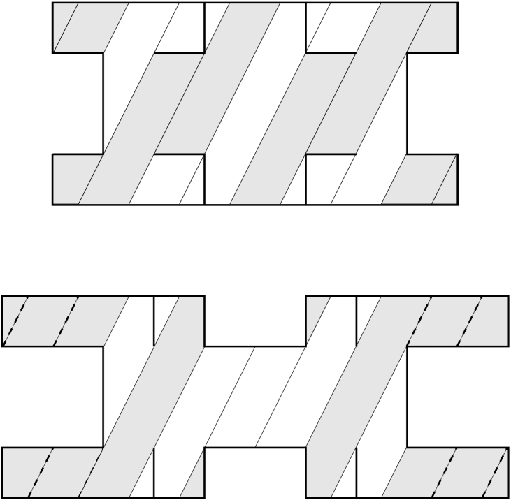
Figure 10: Periodic and diffractive orbits in the unfolded pair of Fig. 7.

V.3 Diffractive orbits

The semiclassical trace formula (72), which is expressed in terms of classical periodic orbits, is only a leading-order approximation for small values of $\hbar$. Higher-order corrections to this formula take into account contributions from diffractive orbits: creeping trajectories, trajectories between scattering points Vattay et al. (1994); Keller (1962); Pavloff and Schmit (1995), and orbits almost tangent to a concave section of the boundary Primack et al. (1997). In the case of polygonal billiards, the semiclassical trace formula (73) has to be corrected to take into account scattering trajectories, that is, classical trajectories going from one scattering point to another, or combinations thereof.

As in the case of periodic orbits, one might believe that the equality of densities $d(E)$ for isospectral billiards must translate to an equality of diffractive orbits. Surprisingly, this is not the case, as we now show. Again, we concentrate on the simple example of polygonal isospectral billiards.

In the case of polygonal billiards, Hannay and Thain (2003) were able to derive an exact expansion for the Green function, as a sum over all scattering trajectories. The exact Green function between a point $a$ and a point $b$ reads

$$G(a,b) = \sum_{n=0}^{\infty}\frac{1}{(2\pi)^{n}}\sum_{\genfrac{}{}{0.0pt}{}{n\ \textrm{vertex}}{\textrm{paths}}}\frac{1}{2i}\int_{-\infty}^{\infty}ds_{1}ds_{2}...ds_{n}$$ (74)

$$\times H_{0}^{(1)}\left[kR(s_{1},s_{2},...,s_{n})\right]$$

$$\times \prod_{k=1}^{n}\frac{2\pi}{(\gamma_{k}M_{k}+\theta_{k}+is_{k})^{2}-\pi^{2}},$$

where

$$R^{2}(s_{1},s_{2},...,s_{n})=\hskip 113.81102pt$$ (75)

$$\left(r_{0}+r_{1}e^{s_{1}}+r_{2}e^{s_{1}+s_{2}}+\cdots+r_{n}e^{s_{1}+s_{2}+\cdots+s_{n}}\right)$$

$$\times\left(r_{0}+r_{1}e^{-s_{1}}+r_{2}e^{-s_{1}-s_{2}}+\cdots+r_{n}e^{-s_{1}-s_{2}-\cdots-s_{n}}\right).$$

The Green function appears as a sum over paths made of $n+1$ straight lines of length $r_{i}$, $0\leq i\leq n$. The first line goes from point $a$ to a diffracting corner, then there are $n$ scattering trajectories going from one diffracting corner to another, and finally a trajectory going from one diffracting corner to point $b$. The diffraction angles are $M_{k}\gamma_{k}+\theta_{k}$, $1\leq k\leq n$, with $\gamma_{k}$ the measure of the angle at the diffracting corner and $M_{k}$ the number of times the path winds around the diffracting corner (thus, $0\leq\theta_{k}<\gamma_{k}$).

Giraud (2004) showed, using the expansion (74) of the Green function, that isospectral domains can be distinguished by the fact that in general the lengths of their diffractive orbits differ. This can be illustrated in the case of the billiard with rectangular base tile unfolded to a translation surface (Fig. 7). If the sides of the base tiles are incommensurate, then there cannot be diffractive orbits of the same length as a given diffractive orbit but in the same direction in the plane. For instance, for the dashed diffractive orbit drawn in the second billiard of Fig. 10, orbits starting from a diffractive corner of the first billiard in the same direction never reach another diffractive corner. This means that the dashed orbit has no partner in the first billiard.

The connection between the energy spectrum and the length spectrum through the trace formula indicates, however, that these discrepancies between diffractive orbits must be compensated in a certain way. This compensation can be understood by analyzing the formula of Hannay and Thain (74). In fact each contribution to the Green function in Eq. (74) has to be understood as an infinite sum over all windings around vertices (see Fig. 11). Here by vertices we mean the four corners and the two points at the middle of the horizontal sides of each of the seven rectangular tiles in Fig. 7.

Figure 11: A contribution to the Green function in the case of forward diffraction. If the orbit goes through a vertex, the term in Eq. (74) should be interpreted as the limit for $\epsilon\to 0$ of an infinite number of trajectories. If there is no vertex only the straight path contribution remains, the other (winding) terms add up to zero.

If there is a diffracting corner (as is the case for instance at the bottom right corner of tile 7 in the second billiard of Fig. 7) then there is a non-zero contribution, while if there is no scatterer (e.g.  at the bottom left corner of tile 7 in the second billiard) the series of diffractive terms adds up to zero,

$$\sum_{M_{k}=-\infty}^{\infty}\frac{2\pi}{(2\pi M_{k}+\pi+is_{k})^{2}-\pi^{2}}=0.$$ (76)

As a consequence, a diffractive contribution to the Green function, going from a point $a$ to a point $b$ through possibly several vertices, has to be understood as a sum of trajectories winding around both scattering and non-scattering vertices (see Fig. 12). Now each of these new “fictitious” trajectories avoids vertices (since they wind around). The reasoning we used in section V.2 applies: With any trajectory one can associate a matrix $M$ describing the edges crossed by the trajectory. The matrix $N$ corresponding to $M$ in the other billiard is such that $TM=NT$, and a partner of the diffractive orbit can be found between tiles $i$ and $j$ such that $N_{ij}=1$.

Thus, even though diffractive orbit lengths might differ, each “expanded” diffractive orbit indeed has a partner of the same length.

Figure 12: A contribution to the Green function in the case of forward diffraction. The filled circles are scattering vertices; the empty ones are non-scattering vertices.

V.4 Green function

This relation between diffractive orbits translates to a relation between Green functions of the two domains Giraud (2004). The matrices $M,N$ introduced in section V.2 verify the property

$$\sum_{i^{\prime},j^{\prime}}T_{ii^{\prime}}T_{jj^{\prime}}M_{i^{\prime}j^{\prime}}=1+2N_{ij},$$ (77)

which can be proved using the commutation relation (7) and the fact that $(T^{2})_{ij}=1+2\delta_{ij}$. Thus, in the expansion (74) of the Green function between a point in tile $i$ and a point in tile $j$ in the first (second) billiard, each trajectory appears with a weight $M_{ij}$ ($N_{ij}$). But according to Eq. (77) we have

$$N_{ij}=\frac{1}{2}\sum_{i^{\prime},j^{\prime}}T_{ii^{\prime}}T_{jj^{\prime}}M_{i^{\prime}j^{\prime}}-\frac{1}{2}.$$ (78)

Therefore from Eq. (74) and identity (78) one can infer a relation between Green functions, namely,

$$G^{(B)}(a,i;b,j)=\frac{1}{2}\sum_{i^{\prime},j^{\prime}}T_{ii^{\prime}}T_{jj^{\prime}}G^{(A)}(a,i^{\prime};b,j^{\prime})-\frac{1}{2}G^{(t)}(a;b),$$ (79)

where $G^{(t)}(a;b)$ is the Green function on the base tile. This relation between Green functions like the relations between periodic orbits or diffractive orbits are all consequences of the transplantation property which is the fundamental feature of all known examples of isospectral billiards.

V.5 Scattering poles of the exterior Neumann problem

In section V.3 we considered the particular case of polygonal isospectral billiards, for which it is possible to express the exact Green function as an infinite expansion given by Eq. (74). In a more general setting, it is also possible to express the Green function of the billiard with Dirichlet boundary conditions as an infinite sum taking into account all possible reflections on obstacles. Balian and Bloch (1974) gave a general method, called “multiple reflection expansion”, which gives the Green function in terms of the free Green function $G_{0}$. Applied to a two-dimensional billiard, this expansion is given by

$$G(q,q^{\prime};E) = G_{0}(q,q^{\prime};E)$$

$$- 2\int_{\partial B}ds\ G_{0}(q,s;E)\partial_{s}G_{0}(s,q^{\prime};E)$$

$$+ (-2)^{2}\int_{\partial B}ds\ ds^{\prime}\ \partial_{s}G_{0}(q,s;E)$$

$$\times \partial_{s^{\prime}}G_{0}(s,s^{\prime};E)G_{0}(s^{\prime},q^{\prime};E)+\cdots,$$

where $s$ and $s^{\prime}$ are points along the boundary, and $\partial_{x}$ denotes the derivative along an outward vector normal to the boundary at point $x$. The first term $G_{0}(q,q^{\prime};E)$ on the right-hand side of Eq. (V.5) corresponds to direct (free) propagation from $q$ to $q^{\prime}$, the first integral corresponds to trajectories from $q$ to $q^{\prime}$ with one reflection on the boundary at point $s$, and so on. We introduce the kernel $K_{E}(q,q^{\prime})=-2\partial_{q^{\prime}}G_{0}(q,q^{\prime};E)$, which is a continuous infinite-dimensional operator defined on $\partial B\times\partial B$ ($\partial B$ is the boundary of the billiard). One can express Eq. (V.5) as

$$G(q,q^{\prime};E)=G_{0}(q,q^{\prime};E)\hskip 142.26378pt$$ (81)

$$-2\sum_{n=0}^{\infty}\int_{\partial B}ds\ ds^{\prime}\ G_{0}(q,s;E)K_{E}^{n}(s,s^{\prime})\partial_{s^{\prime}}G_{0}(s^{\prime},q^{\prime};E).$$

Formal performance of the sum over $n$ yields the infinite-dimensional operator $(\mathbb{I}-K_{E})^{-1}$, where $\mathbb{I}$ is the identity operator. Fredholm theory Smithies (1962) showed that for sufficiently “nice” billiards the operator $(\mathbb{I}-K_{E})^{-1}$ is well-defined and can be expressed as

$$(\mathbb{I}-K_{E})^{-1}=\frac{N_{E}}{D(E)},$$ (82)

where $D(E)$ is the Fredholm determinant $\det(\mathbb{I}-K_{E})$, and $N_{E}$ is an infinite-dimensional operator defined on $\partial B\times\partial B$. The Fredholm determinant admits an expansion

$$D(E)=\sum_{n=0}^{\infty}D_{n}(E),$$ (83)

with $D_{0}(E)=1$, and for $n\geq 1$

$$D_{n}(E)=\frac{(-1)^{n}}{n!}\int_{\partial B}dq_{1}\ldots\int_{\partial B}dq_{n}K\left({\bf q},{\bf q}\right)$$ (84)

(${\bf q}$ is the vector $(q_{1},q_{2},\ldots,q_{n})$). We have introduced the determinant

$$K\left({\bf q},{\bf q}^{\prime}\right)=\left|\begin{array}[]{cccc}K_{E}(q_{1},q_{1}^{\prime})&K_{E}(q_{1},q_{2}^{\prime})&\cdots&K_{E}(q_{1},q_{n}^{\prime})\\ K_{E}(q_{2},q_{1}^{\prime})&K_{E}(q_{2},q_{2}^{\prime})&\cdots&K_{E}(q_{2},q_{n}^{\prime})\\ \cdots&\cdots&\cdots&\cdots\\ K_{E}(q_{n},q_{1}^{\prime})&K_{E}(q_{n},q_{2}^{\prime})&\cdots&K_{E}(q_{n},q_{n}^{\prime})\end{array}\right|.$$ (85)

The operator $N_{E}$ is defined on $\partial B\times\partial B$ by its expansion $N_{E}=\sum_{n=0}^{\infty}N_{n}$ with

$$N_{n}=\sum_{k=0}^{n}D_{k}(E)K_{E}^{n-k}.$$ (86)

The Fredholm determinant $D(E)$ appearing in the expression of the Green function has the property that it has zeros at eigenvalues of the system Georgeot and Prange (1995). A natural question is whether isospectral billiards share the same Fredholm determinant.

It has been shown by Tasaki et al. (1997) that, for billiards with $C^{2}$ boundary, $D(E)$ can be decomposed into an interior and an exterior contribution, namely $D(E)=D(0)d_{\textrm{int}}(E)d_{\textrm{ext}}(E)$. The exterior contribution $d_{\textrm{ext}}(E)$ is related to the scattering of a wave on an obstacle having the shape of the billiard with Neumann boundary conditions, i.e. the zeros of its analytic continuation are resonances of the exterior scattering problem. The interior contribution reads

$$d_{\textrm{int}}(E)=e^{i\frac{\mathcal{A}E}{4}}\left(\frac{\mathcal{L}^{2}E}{4}\right)^{-\frac{\mathcal{A}E}{4\pi}}e^{-\frac{\mathcal{A}\gamma E}{2\pi}}\prod_{n=1}^{\infty}\left(1-\frac{E}{E_{n}}\right)e^{E/E_{n}},$$ (87)

where $\mathcal{A}$ and $\mathcal{L}$ are the area and the perimeter of the billiard, respectively, and $\gamma$ is a constant depending on the geometry of the billiard. The zeros of $d_{\textrm{int}}(E)$ are thus the eigenenergies of the interior Dirichlet problem.

Obviously, isospectral billiards share the same interior part $d_{\textrm{int}}(E)$. But the exterior part depends on the shape of the billiard. In particular solutions of the exterior Neumann scattering problem may differ between two isospectral billiards. Therefore a conclusion of Tasaki et al. (1997) is that isospectral pairs might be distinguished by measuring the sound scattered by them.

To check this property, numerical investigations were performed by Okada et al. (2005a). In fact, Fredholm theory applies only for billiards with a smooth boundary, which is not the case for any of the known examples of isospectral pairs. For billiards with a piecewise smooth boundary, it is however possible to approximate the Fredholm determinant $D(E)$ by a discretized version $D^{m}(E)$, depending on the number $m$ of points taken on the boundary of the billiard, which converges to $D(E)$ for large $m$. This convergence fails for boundaries with corners: All $D^{m}(E)$ tend to 0. Nevertheless, for domains with corners Okada et al. (2005b) showed that it is possible to define a regularized version of $D^{m}(E)$ that converges to $D(E)/D(0)=d_{\textrm{int}}(E)d_{\textrm{ext}}(E)$. Using this regularized version, Okada et al. (2005a) computed numerically zeros of the regularized Fredholm determinant for various pairs of isospectral billiards. It was observed that zeros of the determinant close to the real axis coincide, as they should since they are eigenvalues of the interior problem. On the other hand, complex zeros (remote from the real axis), which correspond to resonances of the exterior Neumann problem, are shown to differ. To quantify this discrepancy between the resonances of the two billiards, the resonance counting number

$$N_{\delta}(r)=\left\{z\in\mathbb{C};|z|<r,-\frac{\pi}{2}<\arg(z)<-\delta\right\}$$ (88)

was studied by Okada et al. (2005a). The best fit $N_{\delta}(r)=C_{\delta,R}r^{2}$, computed over the range $r\in[0,R]$, yields noticeably different values of $C_{\delta,R}$ for each billiard. This clearly shows that isospectral pairs can indeed be distinguished by resonances of scattering waves.

V.6 Eigenfunctions

V.6.1 Triangular states

In general, analytical solutions to the Helmholtz equation $(\Delta+E)\Psi=0$ with Dirichlet boundary conditions cannot be found. However, it is possible to construct particular solutions of this equation provided solutions are known on elementary subdomains. This is, for instance, the case if the subdomains have the shape of a half-square (billiards of Fig. 1), or a rectangle (billiards of Fig. 2).

We take the example of the two billiards in Fig. 1. Each billiard is made of seven triangular (half-square) tiles. Eigenfunctions for a $d\times d$–square with Dirichlet boundary conditions are of the form

$$s_{m,n}(x,y)=\frac{4}{d^{2}}\sin\left(\frac{m\pi x}{d}\right)\sin\left(\frac{n\pi y}{d}\right),$$ (89)

with eigenvalues $E_{m,n}=\pi^{2}(m^{2}+n^{2})/d^{2}$, $m,n\geq 1$. Eigenfunctions for the elementary triangles with Dirichlet boundary conditions are obtained from (89) by antisymmetrization with respect to the diagonal,

$$t_{m,n}(x,y) = \frac{4}{d^{2}}\left[\sin\left(\frac{m\pi x}{d}\right)\sin\left(\frac{n\pi y}{d}\right)\right.$$ (90)

$$- \left.\sin\left(\frac{m\pi y}{d}\right)\sin\left(\frac{n\pi x}{d}\right)\right],$$

and the corresponding eigenenergies are given by $\pi^{2}(m^{2}+n^{2})/d^{2}$, $m>n$. For the sake of definiteness, we consider the two isospectral pairs on a Cartesian reference frame, following Wu et al. (1995), as in Fig. 13. The functions $t_{m,n}$ turn out to be elementary solutions of the Helmholtz equation for both isospectral billiards of Fig. 13.

Figure 13: Isospectral billiards divided into smaller regions.

Indeed $t_{m,n}$ vanishes on all lines $x=kd$, $y=kd$, $y=x+2kd$ and $y=-x+2kd$, $k\in\mathbb{Z}$, which are precisely the lines on which the boundaries of both billiards lie (in the convention of Fig. 13). The particular solutions $t_{mn}$ are called “triangular states”. An example of the lowest-energy triangular state is given in Appendix A.

The labels of the lowest-energy triangular states among the eigenvalues $E_{1}\leq E_{2}\leq\ldots$ of the billiards have been calculated by Gottlieb and McManus (1998). The results are displayed in Table 1.

m	n	Eigenvalue	m	n	Eigenvalue
1	2	$E_{9}$	0	1	$E_{5}$
1	3	$E_{21}$	1	1	$E_{9}$
2	3	$E_{27}$	0	2	$E_{15}$
1	4	$E_{38}$	1	2	$E_{20}$
2	4	$E_{44}$	2	2	$E_{29}$

Table 1: First triangular modes $t_{m,n}$. Left: Dirichlet boundary conditions. Right: Neumann boundary conditions.

Each integer pair $(m,n)$, $m>n$, defines a triangular state $t_{m,n}$. Obviously, the fact that an integer can be represented in more than one way as a sum of two squares leads to degeneracies for triangular states, and hence for the isospectral pairs of Fig. 1.

Note that for Neumann boundary conditions, it can be easily checked that the functions

$$u_{m,n}(x,y) = \frac{4}{d^{2}}\left[\cos\left(\frac{m\pi x}{d}\right)\cos\left(\frac{n\pi y}{d}\right)\right.$$ (91)

$$+ \left.\cos\left(\frac{m\pi y}{d}\right)\cos\left(\frac{n\pi x}{d}\right)\right]$$

for $0\leq m\leq n$, $(m,n)\neq(0,0)$, have a normal derivative that vanishes on all lines $x=kd$, $y=kd$, $y=x+2kd$, and $y=-x+2kd$, $k\in\mathbb{Z}$. Therefore $u_{m,n}$ are solutions of Helmholtz equations for the billiards of Fig. 13 with Neumann boundary conditions. Their label among the eigenstates of the billiards is given in Table 1 Gottlieb and McManus (1998).

V.6.2 Mode-matching method

The knowledge of these particular triangular states is the starting point for the so-called “mode-matching method”. It consists in dividing the billiards into subdomains for which solutions of the Helmholtz equation are known analytically. Consider for example the left billiard of Fig. 13. It is made of five elementary domains, three triangles $A,B,E$ and two squares $C,D$. For each subdomain, analytical solutions for the Dirichlet problem are given by (translations of) functions (89) or (90). We define the function $\psi_{n}(x,y)=\sin(a_{n}x)\sin(b_{n}y)/\sin(b_{n}d)$, where $d$ is the length of the side of the elementary square, and we have set $a_{n}=n\pi/d$ and $b_{n}=\sqrt{E-a_{n}^{2}}$. If given boundary conditions are imposed on the boundaries of these subdomains, as in Fig. 14, solutions can be written explicitly for these elementary subdomains as superpositions of functions obtained from translations or reflections of $\psi_{n}$.

Figure 14: Elementary regions building the isospectral pairs.

In particular, one can construct functions taking the value 0 on the plain boundary and $\sin(a_{n}x)$ ($\sin(a_{n}y)$) on the dashed horizontal (vertical) boundary for each of the domains shown in Fig. 14. Such functions are given by

$$\Phi^{(A)}_{n}(x,y) = \psi_{n}(x,d-y)-\psi_{n}(y,d-x)$$ (92)

$$\Phi^{(B1)}_{n}(x,y) = \psi_{n}(x,y)-\psi_{n}(d-y,d-x)$$

$$\Phi^{(B2)}_{n}(x,y) = \psi_{n}(y,x)-\psi_{n}(d-x,d-y)$$

$$\Phi^{(C1)}_{n}(x,y) = \psi_{n}(y,x)$$

$$\Phi^{(C2)}_{n}(x,y) = \psi_{n}(y,d-x)$$

$$\Phi^{(D1)}_{n}(x,y) = \psi_{n}(y,d-x)$$

$$\Phi^{(D2)}_{n}(x,y) = \psi_{n}(x,d-y)$$

$$\Phi^{(E)}_{n}(x,y) = \psi_{n}(x,y)-\psi_{n}(y,x).$$

The mode-matching method consists in looking for a solution $\Psi$ of the Helmholtz equation as a superposition of such functions, with amplitudes chosen such that $\Psi$ and its partial derivatives be continuous at each boundary between subdomains. At the boundary between elementary subdomains, the eigenfunction $\Psi$ can be expanded on the functions $\varphi_{n}(x)=\sin(a_{n}x)$ as

$$\Psi_{AB}(x,y) = \sum_{n}A_{n}\varphi_{n}(x)$$ (93)

$$\Psi_{BC}(x,y) = \sum_{n}B_{n}\varphi_{n}(y-d)$$

$$\Psi_{CD}(x,y) = \sum_{n}C_{n}\varphi_{n}(y-d)$$

$$\Psi_{DE}(x,y) = \sum_{n}D_{n}\varphi_{n}(x-2d),$$

where the sum goes from 1 to some truncation number $N$. The eigenfunction $\Psi$ is entirely determined by knowledge of the vector ${\bf V}=(A_{1},\ldots,A_{N},B_{1},\ldots,B_{N},C_{1},\ldots,C_{N},D_{1},\ldots,D_{N})$. Therefore $\Psi$ can be written as

$$\Psi_{A}(x,y) = \sum_{n}A_{n}\Phi^{(A)}_{n}(x,y-2d)$$

$$\Psi_{B}(x,y) = \sum_{n}A_{n}\Phi^{(B1)}_{n}(x,y-d)+\sum_{n}B_{n}\Phi^{(B2)}_{n}(x,y-d)$$

$$\Psi_{C}(x,y) = \sum_{n}B_{n}\Phi^{(C1)}_{n}(x-d,y-d)$$

$$+ \sum_{n}C_{n}\Phi^{(C2)}_{n}(x-d,y-d)$$

$$\Psi_{D}(x,y) = \sum_{n}C_{n}\Phi^{(D1)}_{n}(x-2d,y-d)$$

$$+ \sum_{n}D_{n}\Phi^{(D2)}_{n}(x-2d,y-d)$$

$$\Psi_{E}(x,y) = \sum_{n}D_{n}\Phi^{(E)}_{n}(x-2d,y),$$ (94)

where $\Psi_{X}$ is the restriction of the function $\Psi$ to the elementary domain $X=A,B,C,D$, or $E$. The function $\Psi$ is indeed an eigenfunction of the billiard if its normal derivatives at the boundaries between domains are continuous. This latter condition can be written as a system of linear equations that can be cast under the form $M{\bf V}=0$, where $M$ is a $4N\times 4N$-matrix given by

$$M=\left(\begin{array}[]{cccc}U-2W&PWP-PV/2&0&0\\ PWP-PV/2&U-W&-V/2&0\\ 0&-V/2&U&W\\ 0&0&W&U-PWP\end{array}\right)$$ (95)

with $U_{mn}=(b_{n}\cot b_{n}d)\delta_{mn}$, $V_{mn}=(b_{n}/\sin b_{n}d)\delta_{mn}$, $W_{mn}=a_{m}a_{n}/(E-a_{m}^{2}-a_{n}^{2})$, and $P_{mn}=(-1)^{n}\delta_{mn}$. The matrix $M$ depends on $E$ through $b_{n}$. Eigenvalues of the billiard correspond either to values of $E$ where $\det M=0$ or to $V=0$. In the case $V=0$, the wave function vanishes on the boundaries between the domains, and the eigenfunction is a triangular state. If $\det M=0$, Eqs. (V.6.2) give the corresponding eigenfunction.

Interestingly, the mode-matching method provides an alternative proof to isospectrality Wu et al. (1995). The matrix $M^{\prime}$ corresponding to $M$ for the right billiard of Fig. 13 is the $4N\times 4N$-matrix given by

$$M^{\prime}=\left(\begin{array}[]{cccc}U-W&PWP-PV/2&0&0\\ PWP-PV/2&U-W&PV/2&W\\ 0&PV/2&U-W&PWP\\ 0&W&PWP&U-W\end{array}\right).$$ (96)

It can be easily checked that $M$ and $M^{\prime}$ are related by

$$M=^{t}TM^{\prime}T,$$ (97)

with

$$T=\frac{1}{\sqrt{2}}\left(\begin{array}[]{cccc}0&1&0&P\\ 1&0&P&0\\ 0&-1&0&P\\ -1&0&P&0\end{array}\right).$$ (98)

If $\Psi$ is a solution of the Helmholtz equation for the first billiard, it can be written under the form (V.6.2) with constants specified by some vector ${\bf V}$ verifying $M{\bf V}=0$. Let $\Psi^{\prime}$ be the function defined on the second billiard by some constants given by the vector ${\bf V^{\prime}}=T{\bf V}$. Because of Eq. (97) the vector ${\bf V^{\prime}}$ verifies $M^{\prime}{\bf V^{\prime}}=0$, and therefore $\Psi^{\prime}$ is a solution of the Helmholtz equation for the second billiard. Since the relation between $\Psi$ and $\Psi^{\prime}$ is linear, the eigenenergy is the same for both functions, and thus the billiards are isospectral.

V.7 Eigenvalue statistics

As explained in section II, the shape of the elementary building block of a pair of isospectral billiards can be varied at will provided some conditions are satisfied. Thus, examples of chaotic pairs, or pseudo-integrable pairs, or even pairs with a fractal boundary can be produced. However, the most popular examples of isospectral billiards, e.g., those of Fig. 1, are constructed with a triangular-shaped base tile. The resulting billiards are thus polygonal billiards. Billiards with a polygonal boundary can display a whole range of classical behaviors from integrability to chaos. Isospectral billiards made of tiles whose angles are rational multiples of $\pi$ are pseudo-integrable billiards Richens and Berry (1981). The properties of these billiards were mentioned in section II.2.

In the field of quantum chaos, many works have been concerned with a characterization of the statistical properties of spectra of billiards. The question of the spectral properties displayed by polygonal isospectral billiards attracted some interest in the literature. Eigenvalue statistics for the pair of Fig. 1 have been studied numerically by Wu et al. (1995), based on the first 598 energy levels. The short-range correlations of the spectrum were shown to lie between the random matrix statistics of the Gaussian orthogonal ensemble (GOE) and Poisson statistics (see Porter (1965) for a review on the seminal papers, and Guhr et al. (1998) for a recent review on random matrix theory). On removal of the 78 triangular states, it was observed that the nearest-neighbor level spacing distribution function $P(s)$, which characterizes the distribution of the spacings between nearest-neighbor energy levels, agrees with the nearest-neighbor distribution for GOE matrices. The spectral rigidity $\bar{\Delta}_{3}(L)$ (see, e.g., Mehta (1990) for a rigorous definition) measures the deviation of the integrated density of states $N(E)$ (the number of eigenvalues smaller than $E$) from a straight line, on an interval $[E-L/2,E+L/2]$. Computation of $\bar{\Delta}_{3}$ showed that it is also of GOE type for these billiards. Aurich et al. (1997) calculated the functions $E(k,L)$, which give the probability to find $k$ energy levels in an random interval of length $L$ Aurich and Steiner (1990), for isospectral billiards shaped as in Fig. 1, again showing a behavior that is intermediate between the chaotic and integrable cases.

V.8 Nodal domains

Nodal lines for two-dimensional billiards are one-dimensional curves on which eigenfunctions vanish. Nodal domains are connected regions of the billiard where an eigenfunction has a constant sign. A theorem by Courant and Hilbert (1953) states that the $n$th eigenfunction $\Psi_{n}$ has at most $n$ nodal domains. The number $\nu_{n}$ of nodal domains in $\Psi_{n}$ can be further estimated Pleijel (1956). We define a rescaled nodal-domain number $\xi_{n}=\nu_{n}/n\in[0,1]$. If $j_{1}$ is the first zero of the Bessel function $J_{0}$, then $\limsup_{n\to\infty}\xi_{n}\leq(2/j_{1})^{2}$. The limit distribution of $\xi_{n}$ is defined by

$$P(\xi)=\lim_{E\to\infty}\frac{1}{N_{I_{g}(E)}}\sum_{E_{n}\in I_{g}(E)}\delta\left(\xi-\xi_{n}\right),$$ (99)

where $I_{g}(E)$ is the interval $[E,E+gE]$ for some fixed $g>0$, and $N_{I}$ is the number of eigenvalues in the interval $I$. It has been shown by Blum et al. (2002) that this distribution has universal features.

For some instances of isospectral pairs, such as flat tori in $\mathbb{R}^{n}$ with $n\geq 4$ Gnutzmann et al. (2005) (see also Levitin et al. (2006)), it was conjectured that two isospectral domains produce a different number of nodal domains (domains separated by nodal lines where $\Psi=0$). Heuristic arguments as well as numerical investigations were collected by Gnutzmann et al. (2005) to support this conjecture. A recent solution of this conjecture can be found in Bruening et al. (2008).

V.9 Isospectrality versus isolength spectrality

We now consider a related important question. Since transplantation is a mapping between the two billiards, the classical properties should map onto one another as well. Here we investigate the mapping between periodic orbits.

V.9.1 Okada and Shudo’s result on isolength spectrality

Let $D$ be a planar domain obtained by unfolding $N$ times the same triangular building block $B$ with sides $1,2,3$. Then the length spectrum is the set of lengths of closed trajectories (periodic orbits) of $D$. Any periodic orbit on $D$ can be regarded as a “lift” of a closed trajectory on $B$, because its projection is always a periodic orbit on $B$. (The converse is, of course, not necessarily true.) One observes that the number of closed lifts of a given closed trajectory on $B$ is counted as

$$n^{D}(\gamma)=\mbox{Tr}(M^{(\gamma_{m})}M^{(\gamma_{m-1})}\ldots M^{(\gamma_{1})}),$$ (100)

where $\gamma=\prod\gamma_{i}$ ($\gamma_{i}\in\{1,2,3\}$) denotes the sequence representing the order in which a given closed trajectory on $B$ hits the boundary segments. (The $M^{(\gamma_{j})}$’s are adjacency matrices.) Note that such a sequence is not uniquely determined by a given closed orbit — the number of closed lifts, however, is. So the length spectrum of $D$ is determined by the length spectrum of $B$ and by $n^{D}(\gamma)$. Hence, if one considers two domains $D$ and $D^{\prime}$ that are constructed by unfolding the same building block as above, it is sufficient to prove that $n^{D}(\gamma)=n^{D^{\prime}}(\gamma)$ for all possible sequences $\gamma$ in order to deduce “isolength spectrality”.

The following is now obvious.

Theorem V.1 (Okada and Shudo (2001))

Let $D$ and $D^{\prime}$ be two unfolded domains obtained by $N$ times successive reflections of the same building block. If $D$ and $D^{\prime}$ are transplantable, then $n^{D}(\gamma)=n^{D^{\prime}}(\gamma)$ for any sequence $\gamma$, so $D$ and $D^{\prime}$ are isolength spectral.$\blacksquare$

Let $S$ be a finite set, say, $S=\{a_{1},\ldots,a_{k}\}$ with $k\in\mathbb{N}_{0}$. The free group $\mathbf{F}=\mathbf{F}(S)$ generated by $S$ is defined as follows. Introduce a set $S^{-1}:=\{a_{1}^{-1},\ldots,a_{k}^{-1}\}$ which consists of the “inverse symbols” of $S$. A word with alphabet $S$ (or $S\cup S^{-1}$) is just a finite sequence of elements of $S\cup S^{-1}$. A reduced word is a word in which any sequence consisting of an element of $S$ and its inverse is deleted. By definition, $\mathbf{F}$ consists of all reduced words with alphabet $S$, together with the empty word. Group operation is just concatenating words, and reducing if necessary.

Theorem V.2 (Okada and Shudo (2001))

Let $D$ and $D^{\prime}$ be two unfolded domains obtained by $N$ times successive reflections of the same building block. If $n^{D}(\gamma)=n^{D^{\prime}}(\gamma)$ for any sequence $\gamma$, then $D$ and $D^{\prime}$ are transplantable, so also isospectral.

Proof. Let $G$ and $G^{\prime}$ — corresponding to $D$ and $D^{\prime}$, respectively — be the groups generated by the adjacency matrices:

$$G=\langle M^{(\mu)}\rangle,\ \ G^{\prime}=\langle N^{(\mu)}\rangle;$$ (101)

then clearly $G$ and $G^{\prime}$ are subgroups of the symmetric group $\mathbf{S}_{N}$ on $N$ letters. Let $\mathbf{F}_{3}$ be the free group generated by symbols $a,b$ and $c$. Define the surjective homomorphism

$$\Phi_{D}:\mathbf{F}_{3}\mapsto G:\gamma=\gamma_{1}\gamma_{2}\ldots\gamma_{m}\mapsto M^{(\gamma_{m})}M^{(\gamma_{m-1})}\ldots M^{(\gamma_{1})}.$$ (102)

Then

$$G\cong\mathbf{F}_{3}/\mbox{ker}\Phi_{D}\ \ \mbox{and}\ \ G^{\prime}\cong\mathbf{F}_{3}/\mbox{ker}\Phi_{D^{\prime}},$$ (103)

the latter notation being obvious.

Now assume that $n^{D}(\gamma)=n^{D^{\prime}}(\gamma)$ for any sequence $\gamma$. Then

$$\mbox{ker}\,\Phi_{D} = \{\gamma\parallel\Phi_{D}(\gamma)=\mathbb{I}\}=\{\gamma\parallel n^{D}(\gamma)=N\}$$ (104)

$$= \{\gamma\parallel n^{D^{\prime}}(\gamma)=N\}=\{\gamma\parallel\Phi_{D^{\prime}}(\gamma)=\mathbb{I}\}$$

$$= \mbox{ker}\,\Phi_{D^{\prime}}.$$

(Note that $\Phi_{D}(\gamma)$ is a $(0,1)$-matrix, so that $\Phi_{D}(\gamma)=\mathbb{I}$ if and only if $n^{D}(\gamma)=N$.) So the map

$$\Delta:G\mapsto G^{\prime}:\Phi_{D}(\gamma)\mapsto\Phi_{D^{\prime}}(\gamma)$$ (105)

yields an isomorphism between $G$ and $G^{\prime}$.

Let (identity maps)

$$\rho^{D}:G\mapsto\mathbf{GL}(N,\mathbb{C}),\ \ \rho^{D^{\prime}}:G^{\prime}\mapsto\mathbf{GL}(N,\mathbb{C})$$ (106)

be linear representations of $G$ and $G^{\prime}$, respectively. Since the latter groups are isomorphic,

$$\rho=\rho^{D^{\prime}}\circ\Delta:\Phi_{D}(\gamma)\mapsto\Phi_{D^{\prime}}(\gamma)\in\mathbf{GL}(N,\mathbb{C})$$ (107)

is another linear representation of $G$. Since $n^{D}(\gamma)$ and $n^{D^{\prime}}(\gamma)$ become (equal) characters of the representations $\rho^{D}$ and $\rho$ respectively, the representations are similar. So there exists an invertible matrix $T$ for which

$$TM^{(\mu)}=N^{(\mu)}T$$ (108)

for any $\mu$. Thus $D$ and $D^{\prime}$ are transplantable. $\blacksquare$

V.9.2 Penrose–Lifshits mushrooms

Since transplantation implies isolength spectrality, one might wonder if two billiards with the same length spectrum are, in general, necessarily isospectral.

M. Lifshits, exploiting a construction attributed to R. Penrose (see, e.g., Rauch (1978)), constructed a class of pairs of $\mathbb{R}^{2}$-domains that, while not isometric, have periodic geodesics of exactly the same lengths, including multiplicities. When the boundaries are ($C^{\infty}$) smooth, it follows that the two billiards have the same wave invariants, in the sense that the traces of their wave groups, $\,\cos(t\sqrt{\Delta})\,$, differ at most by a smooth function Melrose (1996). Such billiards provide drums that sound different but are similar geometrically.

In this section we describe a construction of smooth Penrose–Lifshits mushroom pairs that are not isospectral, following Fulling and Kuchment (2005). The domains are smooth, so the spectral difference is not attributable to diffraction from corners.

We start from a half-ellipse $E$ with foci $F$ and $F^{\prime}$ as shown in Fig. 15:

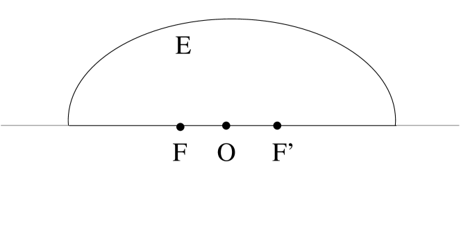
Figure 15: Starting half-ellipse.

The map

$$\xi\mapsto\xi^{\prime},$$ (109)

whether applied to regions, curves, or points, indicates reflection through the minor axis of the ellipse. If objects are interchanged by that reflection, we call them dual. Now replace a line segment by a bounded smooth curve defined over the same interval, $B_{1}$, on the left and $B_{2}$ on the right, with $B_{1}^{\prime}\neq B_{2}\,$, to form a smooth domain $\Omega$ (Fig. 16).

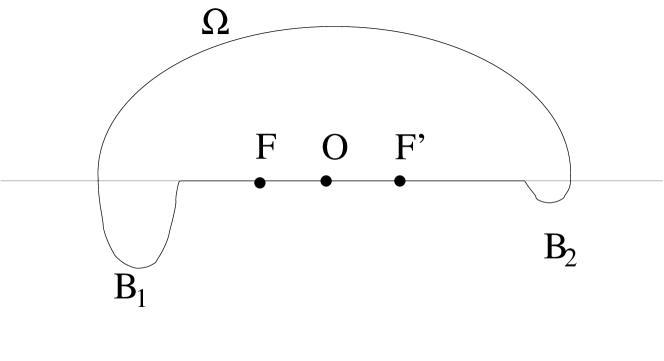
Figure 16: Half-ellipse with two bumps.

Finally, carry out the same replacement operation (not self-dually) between the foci in two dual ways ($M$ and $M^{\prime}$) to get two domains $\Omega_{1}$ and $\Omega_{2}$ (Figs. 17 and 18). We call domains $\Omega_{1}$ and $\Omega_{2}$ constructed in this manner Penrose–Lifshits mushroom pairs.

Figure 17: Perturbed half-ellipse with two bumps.

respectively.

Figure 18: Same as Fig. 17 but perturbed in a dual way.

Theorem V.3 (Fulling and Kuchment (2005))

If $B_{1}$ and $B_{2}$ are given and not dual, then there exist dual bumps $M$ and $\tilde{M}$ such that the resulting Penrose–Lifshits mushrooms $\Omega_{j}$ have the same length spectra and wave invariants but are not isospectral.

Proof. Following Fulling and Kuchment (2005) we first handle the length spectra Melrose (1996); Zelditch (2004b). Geodesics in an ellipse (logically) fall into two disjoint categories Keller and Rubinow (1960); Rauch (1978); Berry (1981): those that intersect the major axis between the foci, and those that do so at or beyond the foci. (The smoothness assumption guarantees that the major axis will not bifurcate in $\Omega_{j}$ by diffraction.)

A similar observation holds for the domains $\Omega_{j}$ just described before Theorem V.3: Any geodesic originating in a curve $B_{1}$ or $B_{2}$ can never reach a curve $M$ or $M^{\prime}$, and vice versa.

The geodesics that do not intersect the focal segment $FF^{\prime}$ are the same for the two domains. Those for $\Omega_{1}$ that do intersect this segment are identified one-to-one with their duals in $\Omega_{2}$ by the reflection. Hence the two billiards are length isospectral. It now suffices to show that it is possible to choose an $M$ in such a way that the two billiards are nonisospectral. One considers the lowest eigenvalue of the domains whose boundary is modified by a small perturbation. Using the Rayleigh–Hadamard formula for change in the spectrum under domain perturbations (cf. Garabedian and Schiffer (1952); Ivanov et al. (1977); Zelditch (2004b) or (Garabedian, 1998, section 15.1, Exercise 9)), one can prove that this eigenvalue is different for the two domains for a given choice of the perturbation. Thus, one can construct non-isospectral billiards having the same length spectrum, and the theorem is proved. $\blacksquare$

V.10 Analytic domains

As all known counterexamples to the question “Can one hear the shape of a drum?” are plane domains with corners, it might be possible that analytic drumheads are spectrally determined. The paper of Zelditch (2009) is part of a series (cf. Zelditch (2004a, c)) devoted to the inverse spectral problem for simply connected analytic Euclidean plane domains $\Omega$, the motivating problem being whether generic analytic Euclidean drumheads are determined by their spectra. The main results of Zelditch (2009) give the strongest evidence to date for this conjecture by proving it for two classes of analytic drumheads: those with an up/down symmetry, and those with dihedral symmetry.

Planar drumheads with symmetry. We now state the results more precisely. As before, by Lsp$(\Omega)$ we denote the length spectrum of $\Omega$, that is, the set of lengths of closed trajectories of its billiard flow. A bouncing ball orbit $\gamma$ is a two-leg periodic trajectory that intersects $\partial\Omega$ orthogonally at both boundary points. By rotating and translating $\Omega$ we may assume that $\gamma$ is vertical, with endpoints at $A=(0,L/2)$ and $B=(0,-L/2)$. Zelditch’s inverse results (Zelditch (2009)) pertain to the following two classes of drumheads, $\mathcal{D}_{1,L}$ and $\mathcal{D}_{m,L}$, which are defined as follows: (i) the class $\mathcal{D}_{1,L}$ of drumheads with one symmetry $\sigma$ and a bouncing ball orbit of length $2L$ which is reversed by $\sigma$, and (ii) the class $\mathcal{D}_{m,L}$ for $m\geq 2$ of drumheads admitting the dihedral group $\mathbf{D}_{2m}$ (acting on $m$ letters) as symmetry group and an invariant $m$-leg reflecting ray.

Note that the class $\mathcal{D}_{1,L}$ consists of simply connected real-analytic plane domains $\Omega$ with the property that there is an isometric involution $\sigma$ of $\Omega$ which “reverses” a nondegenerate bouncing ball orbit (that is, $\sigma(\gamma)=\gamma^{-1}$, i.e. the same orbit reversed) of length $L_{\gamma}=2L$. Other geometric properties can be found in Zelditch (2009).

Let $\mathrm{Spec}_{B}$ denote the spectrum of the Laplacian $\Delta_{B}$ of the domain $\Omega$ with boundary conditions $B$. The result of Zelditch is that for Dirichlet (or Neumann) boundary conditions $B$, the map $\mathrm{Spec}_{B}:\mathcal{D}_{1,L}\mapsto\mathbb{R}^{N}_{+}$ is one-to-one. As a corollary, one obtains the main result of Iantchenko et al. (2002) and Zelditch (1999, 2000) that a simply connected analytic domain with the symmetries of an ellipse and with one axis of a prescribed length $L$ is spectrally determined within this class. The above theorem admits a generalization to the special piecewise analytic mirror symmetric domains with corners that are formed by reflecting the graph of an analytic function, see Zelditch (2009). For $m\geq 2$, that is, “dihedrally symmetric domains”, Zelditch (2009) similarly proves that the map $\mathrm{Spec}_{B}:\mathcal{D}_{m,L}\mapsto\mathbb{R}^{N}_{+}$ is one-to-one.

Higher dimensional drumheads with the symmetry of an ellipsoid. More generally, Hezari and Zelditch (2009) proved that bounded analytic domains $\Omega\subset\mathbb{R}^{n}$ with $\pm$ mirror symmetries across all coordinate axes and with one axis height fixed (and also satisfying some generic non-degeneracy conditions) are spectrally determined among other such domains.  That is, you can hear the shape of a real analytic drum in any number of dimensions if you know in advance that the mystery drums have the symmetries of an ellipsoid. It is one of the first positive higher dimensional inverse spectral results for Euclidean domains that is not restricted to balls.

VI Experimental and Numerical Investigations

Although isospectrality is proved on mathematical grounds, the knowledge of exact eigenvalues and eigenfunctions can not be obtained analytically for such systems. Experimental as well as numerical simulations occurred very early in the history of billiards. In 1909, in the Bulletin international de l’Académie des Sciences de Cracovie, Zaremba proposed a way of “numerically” calculating solutions of the Dirichlet and Neumann problem at a given point Zaremba (1909). To solve the eigenvalue problem for the Helmholtz equation, one standard method is the boundary element method Riddel (1979); Berry and Wilkinson (1984). However, this approach faces problems when the billiard has corners. Such situations have been addressed e.g. by Pisani (1996) and Okada et al. (2005b). The usual numerical methods to compute eigenvalues and eigenfunctions in polygonal billiards are based on the so-called “method of particular solutions” introduced by Fox, Henrici and Moler (FHM) in Fox et al. (1967). At a diffracting corner with angle $\pi\alpha$, a wave function $\Psi$ admits a “corner” decomposition into Bessel functions valid at a distance smaller than to the nearest diffracting corner. In polar coordinates centered around the corner $\pi\alpha$ this decomposition reads

$$\Psi(r,\theta)=\sum_{k}a_{k}J_{k\alpha}(kr)\sin(k\alpha\theta),$$ (110)

where $J_{\nu}$ are Bessel functions of the first kind, and $k=\sqrt{E}$. The sine function in Eq. (110) ensures that the function $\Psi(r,\theta)$ is zero on the boundary edges connected to corner $\pi\alpha$. The idea of FHM is to require that $\Psi$ also vanish on the rest of the boundary at a finite number of points, and to truncate the sum (110). This gives a system of $m$ linear equations, which admits a non-zero solution $\{a_{k},1\leq k\leq m\}$if and only if the matrix corresponding to this linear system is singular. The FHM method therefore consists in varying the energy $E$ and tracking the singularities of the matrix $M$.

Unfortunately, for more than one diffracting corner it becomes virtually impossible to track singularities, especially since in various circumstances the FHM method fails to converge when the number of terms included in Eq. (110) is increased. Even for the paradigmatic pair with half-square base shape (Fig. 1), which is one of the simplest isospectral billiards, each pair has four diffractive angles: two $3\pi/2$ and two $3\pi/4$ angles, and the FHM method fails to give eigenvalues with a good accuracy. This is why attention has been focused on physical experiments.

All known pairs of isospectral billiards are built on the same principle as the ”historical” pair $7_{3}$ of Fig. 1. As explained in section II any initial building block possessing three sides along which to unfold the block can be used to construct an isospectral pair. In particular, the properties of the resulting pair will depend strongly on the choice of the initial building block. Physicists have mainly concentrated on the paradigmatic example of Fig. 1. This allows us to make comparisons between the different approaches.

In this section we review both experimental and numerical investigations which give insight into the behavior of eigenvalues and eigenfunctions for isospectral billiards.

VI.1 Numerical investigations

VI.1.1 Mode-matching method

Numerical approaches to the study of isospectrality for the billiards of Fig. 1 have followed the experiments of Sridhar and Kudrolli that will be reviewed in the next subsection. Various approaches have been used in order to solve the Helmholtz equation $(\Delta+E)\Psi=0$ with Dirichlet boundary conditions inside the billiards. The first numerical results were obtained by Wu, Sprung and Martorell and reported in Wu et al. (1995). Using the mode-matching method described in section V.6.2, they obtained eigenvalues of the billiard as the values for which the determinant of the matrix $M$, given by Eq. (95), vanishes. The results obtained by this method are displayed in column 2 of Table 2. As expected, both billiards yield the same values. The numerical results were found to vary linearly in $1/N$. Wu et al. (1995) compared their results to results obtained by a finite-difference method consisting in discretizing the Laplacian $\Delta$. This finite-difference method gives the results displayed in column 1 of Table 2 (the numerical results are again exactly the same for both billiards). As a check of the validity of this approach, one can identify the eigenvalues of triangular states. The lowest-energy triangular state are expected to have eigenenergies equal to $5\pi^{2}/d^{2}$ and $10\pi^{2}/d^{2}$. As one can see in Table 2, these eigenvalues correspond to the ninth and 21st mode, respectively, consistently with Table 1.

VI.1.2 Expansion of eigenfunctions around the corners with the domain-decomposition method

The main drawback of the mode-matching method of Wu et al. (1995) is the fact that one has to know analytic solutions of the Helmholtz equation on subdomains of the billiard. Driscoll (1997) used a numerical method based on an algorithm by Descloux and Tolley (1983), particularly suited to treating the case of polygonal billiards. The idea is again to decompose the billiard into domains, each domain $\mathcal{D}_{i}$ containing only one diffracting angle $a_{i}$. On each domain the restriction of the eigenfunction $\Psi$ is supposed to be some $\Psi_{i}$ that admits a Bessel function expansion around corner $a_{i}$, according to Eq. (110). Truncation of this expansion to some finite order reduces the problem to that of finding the coefficients of the expansion for the $\Psi_{i}$. Mode-matching numerically leads to undesired singularities. Instead, Descloux and Tolley (1983) used an algorithm minimizing a function that measures discrepancies between the $\Psi_{i}$ and between their derivatives at the boundaries between subdomains. Improvement of this algorithm allowed Driscoll to obtain the first 25 eigenvalues for both billiards of Fig. 1 with an accuracy of up to 12 digits. Betcke and Trefethen (2005) used a modified method of particular solutions using 140 expansion terms at each singular corner, 140 boundary points on each side of the polygon, and 50 interior points to obtain following estimates for the first three eigenvalues: $2.537943999798$, $3.65550971352$ and $5.17555935622$.

VI.2 Experimental realizations

VI.2.1 Electromagnetic waves in metallic cavities

Many experimental studies have been carried out on chaotic quantum billiards to check the various properties conjectured analytically for chaotic systems Bohigas et al. (1984). One commonly used method is based on the correspondence between the stationary Schrödinger equation and the Helmholtz equation for electromagnetic waves in two dimensions (which is also the equation obeyed by vibrating plates). The experiments are carried out by sending electromagnetic microwaves into a cylindrical copper cavity. The height $h$ of the cavity is small, and the two other dimensions are shaped according to the desired billiards to investigate. For wavelengths $\lambda>2h$, i.e. frequencies below $\nu_{0}=c/2h$, all modes obey the two-dimensional wave equation $(\Delta+k^{2})\Psi=0$. The $E_{z}$ component of the electric field plays the role of the quantum wave and vanishes on the boundary. Probes allow one to send an electromagnetic wave into the cavity and to measure the transmission spectrum. In particular, eigenvalues correspond to resonances in the transmission spectrum. Various choices of the probe locations ensure that no resonance is missed.
If $\mathcal{A}$ is the area of the cavity, the number of resonances below $\nu_{0}$ is approximately given by $\frac{\mathcal{A}}{4\pi}(\pi/h)^{2}$. But the quality factor of the cavity is proportional to $h$; therefore one has to find a compromise between a high quality factor and a large number of resonances.
Measurements of the intensity of the wave function (or here the electric field) were achieved by the perturbation body method Sridhar et al. (1992): The resonance frequency of the cavity is shifted by the presence of a small metallic body inside the cavity. This shift is a function of the square of the electric field at the point of the metallic body.

The first experimental investigation of isospectral billiards was realized at Northeastern University, Boston, by Sridhar and Kudrolli (1994). Sridhar and coworkers carried out various studies on chaotic quantum billiards, such as the Sinai billiard (a square billiard with a circular obstacle in the interior), and the Bunimovitch stadium-shaped billiard, observing the scarring of eigenfunctions Sridhar (1991) or localization phenomena Sridhar and Heller (1992) for such billiards. The experiments aimed at investigating isospectrality were realized on cavities having the shape of the isospectral pair of Fig. 1.

Experimentally, each cavity has nine rectangular sides. The base shape is an isosceles rectangular triangle (a half-square) whose smaller side is $d=76$ mm ($3$ in.) long. The height of the cavity is $h=6.3$ mm ($\simeq 0.25$ in.), so that microwaves at frequencies below $\nu_{0}=25$ GHz are actually two-dimensional. Measurements carried out to obtain the 54 lowest eigenvalues showed that, as expected, the eigenvalues of the two cavities are equal. Relative discrepancies of $0.01$ to $0.2\%$ between pairs of eigenvalues were found. These discrepancies and the width of the resonances were assumed to be caused by imperfections due to the assembly of the pieces forming the cavity. This experiment also allowed insight into the properties of eigenvalues of isospectral pairs. It was checked that the eigenvalues found experimentally agree with the Weyl formula (51) for the integrated density of states:

$$\overline{\mathcal{N}}(E)\simeq\frac{\mathcal{A}}{4\pi}E-\frac{\mathcal{L}}{4\pi}\sqrt{E}+\mathcal{K}.$$ (111)

For the choice $d=3$ in. one gets an area $\mathcal{A}=31.5$ in.² and a perimeter $\mathcal{L}=27$ in.; the constant $\mathcal{K}$ is given by Eq. (53) and yields $\mathcal{K}=5/12$. It was observed that at least for the lowest eigenvalues no degeneracy occurred. By measuring the electric field inside the cavity, some of the lowest eigenfunctions were obtained. The results for the ten first eigenvalues are displayed in Table 2. It is interesting to note that these pairs of eigenfunctions look quite different, although they possess the same eigenvalues. It was checked that one eigenfunction could be deduced from the other by transplantation. The particular case of the ninth mode, which is a triangular state, is well reproduced. Indeed, as shown in Table 2, the measured $9$-th eigenvalue is very close to its theoretical value $E=5\pi^{2}/d^{2}$.

Later Dhar et al. (2003) applied a similar technique to a chaotic isospectral billiard made of the billiard with half-square base tile with scattering circular disks inside, showing experimentally that isospectrality is indeed retained, provided scatterers are added in a way consistent with the unfolding rules.

VI.2.2 Transverse vibrations in vacuum for liquid crystal smectic films

Another experimental realization of Kac’s membranes was achieved using liquid crystal films in a smectic phase, spanning a shape of the form of the isospectral billiard Even and Pieranski (1999). First, the shapes were etched in circular stainless-steel wafers of diameter 4cm and thickness 125 $\mu$m. The smectic film is then drawn on the shape, and after a few hours it reaches an equilibrium with uniform thickness $e$ of several hundred nanometers (corresponding to a few dozens monomolecular layers) over the whole surface. The whole experiment is set in vacuum. The film then obeys the wave equation

$$\gamma\Delta z=\rho e\frac{\partial^{2}z}{\partial t^{2}},$$ (112)

where $\gamma$ is the intrinsic tension of the film (in the experiments $\gamma\sim 5.10^{-2}$N/m), and $\rho$ is the density, with a vertical displacement $z$ vanishing on the border. The film is excited by a voltage applied by an electrode under the film, and the amplitude and phase of its oscillations are measured by sending in a laser beam and measuring its deviations with a photodiode. The signal detected is proportional to the height of the film at the position of the electrode. The frequency of the excitation is varied from a few Hertz to several kiloHertz, and eigenfrequencies correspond to resonance peaks. Displacing the electrode over the whole shape allows to reconstruct eigenmodes.

The experiment was carried out on isospectral billiards with an isosceles triangular base shape: two angles $\beta=\gamma$ are equal, while the third one is varied from $\alpha=67.5^{\circ}$ to $97.5^{\circ}$. The angle $\alpha=90^{\circ}$ corresponds to the example of Fig. 1. The first 30 modes for both shapes were measured. The average relative difference between two eigenvalues for a given mode is 0.3$\%$, which is within the estimated experimental error of order 0.5$\%$. For the right angle triangle ($\alpha=90^{\circ}$) the modes can be compared with other numerical or experimental results. Data for the ten first eigenvalues of the $\alpha=90^{\circ}$ billiards were given by Even and Pieranski (1999) and are displayed in Table 2. When the parameter $\alpha$ is varied, there is an avoided crossing between eigenvalues of the eighth and ninth mode. Since the ninth mode is a triangular mode (see section V.6.1) and the eighth is not, the coupling between these two modes necessarily comes from experimental imperfections.

This experiment has also been tested on a billiard where the gluing scheme of the base triangles is modified. That is, tile $E$ in Fig. 13 (left) is flipped around the line $x=5d/2$. This leads to a significantly different spectrum. In particular, the triangular modes are no longer eigenstates of such a billiard. Again this is a check that the way the tiles are glued together, according to the rules constructed from finite projective spaces or from Sunada triples, is of primary importance for isospectrality.

rank	Finite differences	Mode matching	Electromagnetic waves		Smectic films (relative values)
1	1.028936	1.028535	1.02471	1.02481	1.000000	1.000000
2	1.481865	1.481467	1.46899	1.47194	1.438000	1.430000
3	2.098249	2.097467	2.08738	2.08831	2.040000	2.027000
4	2.649715	2.649547	2.64079	2.63985	2.571000	2.548000
5	2.938176	2.937434	2.93297	2.92949	2.854000	2.823000
6	3.732689	3.732334	3.72695	3.71892	3.623000	3.570000
7	4.295193	4.294728	4.28393	4.28388	4.184000	4.153000
8	4.677665	4.677532	4.67021	4.66917	4.554000	4.507000
9	5.000002	5.000000	4.98838	4.98531	4.861000	4.811000
10	5.291475	5.290275	5.27908	5.27278	5.150000	5.095000
11	5.801531	5.801138	5.78755	5.78371
12	6.433894	6.432156	6.41357	6.43781
13	6.866260	6.866226	6.84891	6.84718
14	7.159802	7.159343	7.15242	7.16045
15	7.694737	7.692417	7.67783	7.70604
16	8.463655	8.463257	8.44285	8.45947
17	8.613536	8.611169	8.57859	8.62220
18	9.012405	9.010349	8.99495	8.97209
19	9.609968	9.609791	9.60312	9.59562
20	9.921131	9.921040	9.92583	9.93689
21	10.000008	10.000000	10.00330	10.03932
22	10.571020	10.569736	10.55227	10.55740
23	11.066916	11.065727	11.09578	11.10035
24	11.419551	11.418850	11.41874	11.40569
25	11.984650	11.984080	11.99364	11.98033

Table 2: Comparison between the first eigenvalues $E_{i}$ of the isospectral pair obtained by various methods, expressed in units of $\pi^{2}/d^{2}$. The ninth mode corresponds to the triangular mode: its normalized eigenvalue is expected to be equal to 5. (The conversion from frequencies to lengths is done assuming vacuum in the cavity; Wu et al. (1995) gave the values for electromagnetic cavities with a factor of 1.0006 corresponding to the presence of air in the cavity.)

VI.2.3 Isospectral electronic nanostructures

Recently Moon et al. (2008) an experiment was done involving electrons confined in isospectral billiards, with the purpose of using transplantation to reconstruct the quantum phase of measured wavefunctions. Each billiard consisted of a wall of 90 CO molecules, constructed by positioning the molecules with the tip of a scanning tunneling microscope. The chosen billiards were built according to the pattern of Fig. 1, but the base shape was chosen to be a triangle with angles $(\pi/2,\pi/3,\pi/6)$. As in Even and Pieranski (1999), it was checked that billiards violating the isospectral construction rule led to a different result.

Amusingly, Moon et al. (2008) took Kac’s question literally by converting the average measured spectra into audio frequencies, checking that one could indeed ”hear” non-isospectrality.

VII Sunada Theory

The examples of isospectral billiards considered so far can be proved to be isospectral by quite simple tools. However historically they were constructed by a group-theoretical approach. The mathematical theory of isospectrality rests on a theory by Sunada. We first review the necessary basic notions of group theory. Then, in section VII.5, we introduce Sunada Theory.

VII.1 Permutations

Following the usual conventions, we denote permutation action exponentially (i.e. the image of an element $x$ by the permutation $g$ is $x^{g}$) and let elements act on the right. We denote the identity element of a group by $\mathbf{id}$ or $\mathbf{1}$, if no special symbol has been introduced for it before. A group $G$ without its identity $\mathbf{id}$ is denoted $G^{\times}$. The number of elements of a group $G$ is denoted by $|G|$. A permutation group $(G,X)$ is a pair consisting of a group $G$ and a set $X$ such that each element $g$ of $G$ defines a permutation $g:X\rightarrow X$ of $X$, and the permutation defined by the product $gh$, $g,h\in G$, is given by $gh:X\rightarrow X:x\mapsto(x^{g})^{h}$. An involution in a group is an element $g$ of order $2$, that is, such that $g^{2}=\mathbf{id}$.

VII.2 Commutator notions

The group-theoretic setting of Sunada theory requires introduction of some notions such as the commutator of two groups and perfect groups. The conjugate of $g$ by $h$ is $g^{h}=h^{-1}gh$. Let $H$ be a group. The commutator of two group elements $g,h$ is equal to $[g,h]=g^{-1}h^{-1}gh$. The commutator of two subsets $A$ and $B$ of a group $G$ is the subgroup $[A,B]$ generated by all elements $[a,b]$, with $a\in A$ and $b\in B$. The commutator subgroup of $G$ is $[G,G]$, also denoted by $G^{\prime}$. Two subgroups $A$ and $B$ centralize each other if $[A,B]=\{\mathbf{id}\}$. The subgroup $A$ normalizes $B$ if $B^{a}=B$ for all $a\in A$, which is equivalent to $[A,B]$ being a subgroup of $B$. If $A$ and $B$ are two subgroups of the group $G$, then they are conjugate(d) if there is an element $g$ of $G$ such that $A^{g}=B$. The subgroup $A$ of $G$ is (a) normal (subgroup) in (of) $G$ if $A^{g}=A$ for all $g\in G$. In such a case, we write $A\unlhd G$. If $A\neq G$, we also write $A\lhd G$.

Inductively, we define the $n$th central derivative $[G,G]_{[n]}$ of a group $G$ as $[G,[G,G]_{[n-1]}]$, and the $n$th normal derivative $[G,G]_{(n)}$ as $[[G,G]_{(n-1)},[G,G]_{(n-1)}]$. For $n=0$, the zeroth central and normal derivatives are by definition equal to $G$ itself. If, for some natural number $n$, $[G,G]_{(n)}=\{\mathbf{id}\}$, and $[G,G]_{(n-1)}\neq\{\mathbf{id}\}$, then we say that $G$ is solvable (soluble) of length $n$. If $[G,G]_{[n]}=\{\mathbf{id}\}$ and $[G,G]_{[n-1]}\neq\{\mathbf{id}\}$, then we say that $G$ is nilpotent of class $n$. The center of a group is the set of elements that commute with every other element, i.e., $Z(G)=\{z\in G\parallel[z,g]=\mathbf{id},\forall g\in G\}$. Clearly, if a group $G$ is nilpotent of class $n$, then the $(n-1)$th central derivative is a nontrivial subgroup of $Z(G)$.

A group $G$ is the central product of its subgroups $A$ and $B$ if $AB=G$, $A\cap B$ is contained in the center of $G$, and $A$ and $B$ centralize each other. Sometimes we write $G=A\circ B$ in such a case.

A group $G$ is called perfect if $G=[G,G]=G^{\prime}$.

Let $R$ be a finite group. The Frattini group $\phi(R)$ of $R$ is the intersection of all proper maximal subgroups, or is $R$ if $R$ has no such subgroups.

VII.3 Finite simple groups

A group is simple if it does not contain nontrivial normal subgroups.

The finite simple groups are often regarded as the elementary particles in finite group theory. Before we explain this more precisely, recall that a composition series of a group $G$ is a normal series

$$1=H_{0}\lhd H_{1}\lhd\cdots\lhd H_{n}=G,$$ (113)

such that each $H_{i}$ is a maximal normal subgroup of $H_{i+1}$. Equivalently, a composition series is a normal series such that each factor group $H_{i+1}/H_{i}$ is simple. The factor groups are called composition factors.

A normal series is a composition series if and only if it is of maximal length. That is, there are no additional subgroups that can be “inserted” into a composition series. The length $n$ of the series is called the composition length.

If a composition series exists for a group $G$, then any normal series of $G$ can be refined to a composition series. Furthermore, every finite group has a composition series.

A group may have more than one composition series. However, the Jordan-Hölder theorem states that any two composition series of a given group are equivalent.

The classification of finite simple groups (see Solomon (2001) for a survey) states that every finite simple group is cyclic, or alternating, or is contained in one of $16$ families of groups of Lie type (including the Tits group, which strictly speaking is not of Lie type), or one of $26$ sporadic groups.

Conway et al. (1985) provided a list of the finite simple groups, see also (Gorenstein, 1980, p. 490-491). In this review, we encounter several aspects of certain simple groups in the construction theory of counter examples to Kac’s initial question.

VII.4 $p$-Groups and extra-special groups

The present section will be useful for construction of examples in section VII.6.

For a prime number $p$, a $p$-group is a group of order $p^{n}$ for some natural number $n\neq 0$. A Sylow $p$-subgroup of a finite group $G$ is a $p$-subgroup of order $p^{n}$ such that $p^{n+1}$ does not divide $|G|$.

A $p$-group $P$ is special if either $[P,P]=Z(P)=\phi(P)$ is elementary Abelian or $P$ itself is. (A group is elementary Abelian if it is Abelian, and if there exists a prime $p$ such that each of its nonidentity elements has order $p$.) Note that $P/[P,P]$ is elementary Abelian in that case. So

$$P/[P,P]\cong V(n,p),$$ (114)

where $V(n,p)$ is the $n$-dimensional vector space over $\mathbb{F}_{p}$ (here seen as its additive group), and $|P|=p^{n}|[P,P]|$.

Hence we have the exact sequence

$$\mathbf{1}\mapsto[P,P]\mapsto P\mapsto V(n,p)\mapsto\mathbf{1}.$$ (115)

If furthermore $|Z(P)|=|[P,P]|=|\phi(P)|=p$, $P$ is called extra-special.

We now present a classification for extra-special groups that depends on the knowledge of the nonabelian $p$-groups of order $p^{3}$.

There are four nonabelian $p$-groups of order $p^{3}$ — see Gorenstein (1980). First we have $M=M(p)$:

$$M(p) = \langle x,y,z\parallel x^{p}=y^{p}=z^{p}=\mathbf{1},$$ (116)

$$[x,z]=[y,z]=\mathbf{1},[x,y]=z\rangle.$$

(Note that this is the general Heisenberg group of order $p^{3}$ which we will encounter later on.) Next, define

$$M_{3}(p)=\langle x,y\parallel x^{p^{2}}=y^{p}=\mathbf{1},x^{y}=x^{p+1}\rangle.$$ (117)

Finally, we have the dihedral group $D$ of order $8$ and the generalized quaternion group $Q$ of order $8$.

Theorem VII.1 (Gorenstein (1980))

An extra-special $p$-group $P$ is the central product of $r\geq 1$ nonabelian subgroups of order $p^{3}$. Moreover, we have the following.

• If $p$ is odd, $P$ is isomorphic to $N^{k}M^{r-k}$, while if $p=2$, $P$ is isomorphic to $D^{k}Q^{r-k}$ for some $k$. In either case, $|P|=p^{2r+1}$.

• If $p$ is odd and $k\geq 1$, $N^{k}M^{r-k}$ is isomorphic to $NM^{r-1}$, the groups $M^{r}$ and $NM^{r-1}$ are not isomorphic and $M^{r}$ is of exponent $p$.

• If $p=2$, then $D^{k}Q^{r-k}$ is isomorphic to $DQ^{r-1}$ if $k$ is odd and to $Q^{r}$ if $k$ is even, and the groups $Q^{r}$ and $DQ^{r-1}$ are not isomorphic.

(All the products considered are central products.)

VII.5 Sunada Theory

We now turn to the main theorems of Komatsu and Sunada, which allowed Gordon et al. to produce the first known example of isospectral billiards. Sunada’s idea was to reduce the problem of finding isospectral manifolds to a group-theoretical problem, namely, constructing triplets of groups having a certain property. As the groups that appear in Sunada’s proof are Galois groups, we need some more definitions.

A field extension $\mathbb{L}/\mathbb{K}$ is called algebraic if every element of L is algebraic over $\mathbb{K}$, i.e., if every element of $\mathbb{L}$ is a root of some non-zero polynomial with coefficients in $\mathbb{K}$. (Field extensions which are not algebraic, i.e. which contain transcendental elements, are called transcendental.)

Let $\mathbb{K}$ be an algebraic number field of degree $n$. Recall that a number field is a finite, algebraic field extension of $\mathbb{Q}$; its degree is the dimension over $\mathbb{Q}$ as a $\mathbb{Q}$-vector space. A standard example is $\mathbb{Q}(\sqrt{2})$.

The ring of integers of an algebraic number field $\mathbb{K}$, often denoted by $O_{\mathbb{K}}$, is the ring of algebraic integers contained in $\mathbb{K}$. An algebraic integer is an element of $\mathbb{K}$ that is a root of some monic polynomial with coefficients in $\mathbb{Z}$.

The (Dedekind) zeta function $\zeta_{\mathbb{K}}(s)$ (associated with $\mathbb{K}$), $s$ being a complex variable, is defined by

$$\zeta_{\mathbb{K}}(s)=\sum_{I}[N_{Q}^{\mathbb{K}}(I)]^{-s},$$ (118)

taken over all ideals $I$ of the ring of integers $O_{\mathbb{K}}$ of $\mathbb{K}$, $I\neq\{0\}$. Note that $N_{Q}^{\mathbb{K}}(I)$ denotes the norm of $I$ (to $\mathbb{Q}$), equal to $|O_{\mathbb{K}}/I|$.

An ideal $P$ of a ring $R$ is a prime ideal if it is a proper ideal and if for any two ideals $A$ and $B$ in $R$ such that $AB\subseteq P$, we have that $A\subseteq P$ or $B\subseteq P$. Let $p$ be a rational prime. Let $P_{1},\ldots,P_{g}$ be the prime ideals of $O_{\mathbb{K}}$ lying above $p$. Then

$$\langle p\rangle=\prod_{i=1}^{g}P_{i}^{e_{i}},$$ (119)

where

$$e_{i}=e_{\mathbb{K}}(P_{i}).$$ (120)

Here $e_{\mathbb{K}}(P_{i})$ is the ramification index of $P_{i}$ over $\mathbb{K}$. If $e_{i}>1$ for some $i\in\{1,\ldots,g\}$, then $p$ is said to be ramified in $\mathbb{K}$. If $e_{i}=1$ for all $i$, $p$ is unramified in $\mathbb{K}$.

The conjugate elements of an algebraic element $\alpha$, over a field $\mathbb{K}$, are the roots of the minimal polynomial of $\alpha$ over $\mathbb{K}$. (For example, the cubic roots of 1 are $1,-1/2+\sqrt{3}/2i,-1/2-\sqrt{3}/2i$. The latter two roots are conjugate elements in the field $\mathbb{K}=\mathbb{Q}[\sqrt{-3}]$.)

Let $\mathbb{K}=\mathbb{Q}(\theta)$ be as above, that is, an algebraic number field of degree $n$ ($\theta\in\mathbb{C}$). Suppose $\theta_{1},\theta_{2},\ldots,\theta_{n}$ are the conjugates of $\theta$ over $\mathbb{Q}$. If

$$\mathbb{Q}(\theta_{1})=\cdots=\mathbb{Q}(\theta_{n})=\mathbb{K},$$ (121)

then $\mathbb{K}$ is a Galois extension of $\mathbb{Q}$.

Suppose that $\mathbb{E}$ is an extension of the field $\mathbb{F}$ (written as $\mathbb{E}/\mathbb{F}$). Consider the set of all automorphisms of $\mathbb{E}/\mathbb{F}$ (that is, isomorphisms $\alpha$ from $\mathbb{E}$ to itself such that $\alpha(x)=x$ for every $x\in\mathbb{F}$). This set of automorphisms with the operation of function composition forms a group, sometimes denoted by $\mathrm{Aut}(\mathbb{E}/\mathbb{F}$). If $\mathbb{E}/\mathbb{F}$ is a Galois extension, then $\mathrm{Aut}(\mathbb{E}/\mathbb{F}$) is called the Galois group of (the extension) $\mathbb{E}$ over $\mathbb{F}$, and is usually denoted by $\mathrm{Gal}(\mathbb{E}/\mathbb{F}$).

A number-theoretic exercise which asks for non-isomorphic number fields $\mathbb{K}_{1}$ and $\mathbb{K}_{2}$ with the same zeta function has the following answer:

Theorem VII.2 (Komatsu (1976))

Let $\mathbb{K}$ be a finite Galois extension of $\mathbb{Q}$ with Galois group $G=\mathrm{Gal}(\mathbb{K}/\mathbb{Q})$, and let $\mathbb{K}_{1}$ and $\mathbb{K}_{2}$ be the subfields of $\mathbb{K}$ corresponding to subgroups $G_{1}$ and $G_{2}$ of $G$, respectively. Then the following conditions are equivalent:

• Each conjugacy class of $G$ meets $G_{1}$ and $G_{2}$ in the same number of elements;

• The same primes $p$ are ramified in $\mathbb{K}_{1}$ and $\mathbb{K}_{2}$ and for the unramified $p$ the decomposition of $p$ in $\mathbb{K}_{1}$ and $\mathbb{K}_{2}$ is the same;

• The zeta functions of $\mathbb{K}_{1}$ and $\mathbb{K}_{2}$ are the same.

In particular, if $G_{1}$ and $G_{2}$ are not conjugate in $G$, then $\mathbb{K}_{1}$ and $\mathbb{K}_{2}$ are not isomorphic while having the same zeta function. It should be noted that several such triples $(G,G_{1},G_{2})$ are known — see the examples in this section.

Any group triple $(G,G_{1},G_{2})$ satisfying Theorem VII.2(i) is said to satisfy “Property (*)”.

Sunada’s idea was to establish a counterpart of this theorem for Riemannian geometry. In that context, there is an analogue for the Dedekind zeta function. For $\mathfrak{M}$ a Riemannian manifold, one defines

$$\zeta_{\mathfrak{M}}(s)=\sum_{i=1}^{\infty}\lambda_{i}^{-s},\ \ \mathfrak{Re}(s)\gg 0,$$ (122)

where

$$0<\lambda_{1}\leq\lambda_{2}\leq\cdots$$ (123)

are the non-zero eigenvalues of the Laplacian for $\mathfrak{M}$. The function $\zeta_{\mathfrak{M}}$ has an analytic continuation to the whole plane, and it is well-known that $\zeta_{\mathfrak{M}_{1}}(s)=\zeta_{\mathfrak{M}_{2}}(s)$ if and only if $\mathfrak{M}_{1}$ and $\mathfrak{M}_{2}$ are isospectral.

The following theorem gives sufficient conditions for two manifolds to have the same zeta function.

Theorem VII.3 (Sunada (1985))

Let $\pi:\mathfrak{M}\mapsto\mathfrak{M}_{0}$ be a normal finite Riemannian covering with covering transformation group $G$, and let $\pi_{1}:\mathfrak{M}_{1}\mapsto\mathfrak{M}_{0}$ and $\pi_{2}:\mathfrak{M}_{2}\mapsto\mathfrak{M}_{0}$ be the coverings corresponding to the subgroups $H_{1}$ and $H_{2}$ of $G$, respectively. If the triplet $(G,H_{1},H_{2})$ satisfies Property (*), then the zeta functions $\zeta_{\mathfrak{M}_{1}}(s)$ and $\zeta_{\mathfrak{M}_{2}}(s)$ are identical.

The proof of the latter theorem makes use of an interesting trace formula, which we present now.

If $A$ is a non-negative self-adjoint operator of a Hilbert space, one defines the trace of $A$ as an extended real number by the possibly divergent sum $\sum_{k}\langle Ae_{k},e_{k}\rangle$, where $\{e_{j}\}_{j}$ is an orthonormal base of the space. It is of trace class if and only if $\mathrm{Tr}(A)<\infty$.

Let $V$ be a Hilbert space on which a finite group $G$ acts as unitary transformations and let $A:V\mapsto V$ be a self-adjoint operator of trace class such that $A$ commutes with the $G$-action. For a subgroup $H$ of $G$, denote by $V^{H}$ the subspace of $H$-invariant vectors.

Trace Formula. The restriction of $A$ to the subspace $V^{G}$ is also of trace class, and

$$\mbox{tr}(A|_{V^{G}})=\sum_{[g]\in[G]}(|G_{g}|)^{-1}\mbox{tr}(gA),$$ (124)

where $[G]=\{[g]\}$, $[g]$ is the conjugacy class of $g$ in $G$ and $G_{g}$ is the centralizer of $g$ in $G$.

If the triplet $(G,G_{1},G_{2})$ satisfies Property (*), then

$$\mbox{tr}(A|_{V^{G_{1}}})=\mbox{tr}(A|_{V^{G_{2}}}).$$ (125)

Even if $G_{1}$ and $G_{2}$ are not conjugate, the manifolds $\mathfrak{M}_{1}$ and $\mathfrak{M}_{2}$ could possibly be isometric.

Theorem VII.4 (Sunada (1985))

There exist finite coverings $\pi_{1}:\mathfrak{M}_{1}\mapsto\mathfrak{M}_{0}$ and $\pi_{2}:\mathfrak{M}_{2}\mapsto\mathfrak{M}_{0}$ of Riemann surfaces with genus $\geq 2$ such that for a generic metric $g_{0}$ on $\mathfrak{M}_{0}$, the surfaces $(\mathfrak{M}_{1},\pi_{1}^{*}g_{0})$ and $(\mathfrak{M}_{2},\pi_{2}^{*}g_{0})$ are isospectral, but not isometric.

Sunada’s theorem allows us to construct isospectral pairs provided we find triples $(G,G_{1},G_{2})$ satisfying Property (*) — “Sunada triples”.

Now we give examples of such triples.

VII.6 Examples of Sunada triples

Example 1 — see Gerst (1970). Let $G$ be the semidirect product $\mathbb{Z}/8\mathbb{Z}^{\times}\ltimes\mathbb{Z}/8\mathbb{Z}$, and define $G_{1}$ and $G_{2}$ by

$$G_{1} = \{(1,0),(3,0),(5,0),(7,0)\},$$

$$G_{2} = \{(1,0),(3,4),(5,4),(7,0)\}.$$ (126)

Example 2 — see Gassmann (1926). Let $G=\mathbf{S}_{6}$ be the symmetric group on six letters $\{a,b,c,d,e,f\}$. Set

$$G_{1}=\{\mathbf{1},(ab)(cd),(ac)(bd),(ad)(bc)\}$$ (127)

and

$$G_{2}=\{\mathbf{1},(ab)(cd),(ab)(ef),(cd)(ef)\}.$$ (128)

Example 3 — see Komatsu (1976). Let $G_{2}$ and $G_{2}$ be two finite groups with the same order, and suppose that their exponents (equal to the least common multiples of the orders of their elements) both equal the same odd prime $p$. Set $|G_{1}|=|G_{2}|=p^{h}$ for $h\in\mathbb{N}^{\times}$ and embed $G_{1}$ and $G_{2}$ in the symmetric group $\mathbf{S}_{p^{h}}$ on $p^{h}$ letters by their left action on themselves. For a conjugacy class $[g]$ corresponding to the partition

$$|\mathbf{S}_{p^{h}}|=p^{h}!=p+p+\cdots+p,$$ (129)

we have

$$|([g]\cap G_{1})|={p^{h}}-1=|([g]\cap G_{2})|,$$ (130)

while $|([g]\cap G_{i})|=0$ otherwise.

Concretely, let $G_{1}=(\mathbb{Z}/p\mathbb{Z})^{3}$, and let $G_{2}$ be the group

$$G_{2}=\langle a,b\parallel a^{p}=b^{p}=[a,b]^{p}=\mathbf{1},\hskip 56.9055pt$$

$$a[a,b]=[a,b]a,b[a,b]=[a,b]b\rangle,\hskip 28.45274pt$$ (131)

that is, $G_{2}$ is the extra-special group of order $p^{3}$. Then $(\mathbf{S}_{p^{3}},G_{1},G_{2})$ verifies Property (*).

One can in fact generalize Komatsu’s example by defining the following group. The general Heisenberg group $\mathbf{H}_{n}$ of dimension $2n+1$ over $\mathbb{F}_{q}$, with $n$ a natural number, is the group of square $(n+2)\times(n+2)$-matrices with entries in $\mathbb{F}_{q}$, of the following form (and with the usual matrix multiplication):

$$\left(\begin{array}[]{ccc}1&\alpha&c\\ 0&\mathbb{I}_{n}&\beta^{T}\\ 0&0&1\\ \end{array}\right),$$ (132)

where $\alpha,\beta\in\mathbb{F}_{q}^{n}$, $c\in\mathbb{F}_{q}$, and with $\mathbb{I}_{n}$ the $n\times n$-unit matrix. Let $\alpha,\alpha^{\prime},\beta,\beta^{\prime}\in\mathbb{F}_{q}^{n}$ and $c,c^{\prime}\in\mathbb{F}_{q}$; then

$$\left(\begin{array}[]{ccc}1&\alpha&c\\ 0&\mathbb{I}_{n}&\beta^{T}\\ 0&0&1\\ \end{array}\right)\times\left(\begin{array}[]{ccc}1&\alpha^{\prime}&c^{\prime}\\ 0&\mathbb{I}_{n}&{\beta^{\prime}}^{T}\\ 0&0&1\\ \end{array}\right)\hskip 56.9055pt$$ (139)

$$=\left(\begin{array}[]{ccc}1&\alpha+\alpha^{\prime}&c+c^{\prime}+\langle\alpha,\beta^{\prime}\rangle\\ 0&\mathbb{I}_{n}&\beta+\beta^{\prime}\\ 0&0&1\\ \end{array}\right).\hskip 14.22636pt$$ (143)

Here $\langle x,y\rangle$, with $x=(x_{1},x_{2},\ldots,x_{n})$ and $y=(y_{1},y_{2},\ldots,y_{n})$ elements of $\mathbb{F}_{q}^{n}$, denotes $x_{1}y_{1}+x_{2}y_{2}+\ldots+x_{n}y_{n}$.

The following properties hold for $\mathbf{H}_{n}$.

• $\mathbf{H}_{n}$ has exponent $p$ if $q=p^{h}$ with $p$ an odd prime; it has exponent $4$ if $q$ is even.

• The center of $\mathbf{H}_{n}$ is given by

  $$\{(0,c,0)\parallel c\in\mathbb{F}_{q}\}.$$ (144)

• $\mathbf{H}_{n}$ is nilpotent of class $2$.

Then, as above, $(\mathbf{S}_{p^{2n+1}},\mathbf{H}_{n},(\mathbb{Z}/p\mathbb{Z})^{2n+1})$ verifies Property (*).

Any finite group arises as the fundamental group of a compact smooth manifold of dimension $4$. For a triplet $(G,G_{1},G_{2})$ of the type described in Example 3, we find a compact manifold $\mathfrak{M}_{0}$ with fundamental group $G$. Let $\mathfrak{M}$ be the universal covering of $\mathfrak{M}_{0}$. Then the quotients $\mathfrak{M}_{i}=\mathfrak{M}/G_{i}$ have non-isomorphic fundamental groups $G_{i}$, $i=1,2$. By Theorem VII.3 the manifolds $(\mathfrak{M}_{1},\pi_{1}^{*}g_{0})$ and $(\mathfrak{M}_{2},\pi_{2}^{*}g_{0})$ are isospectral for any metric $g_{0}$ on $\mathfrak{M}_{0}$, but not isometric.

VIII Related Questions

The literature on isospectrality is large, and it is out of the question to review the entire field. In the present paper we have concentrated on the questions addressed by planar two-dimensional domains with Dirichlet boundary conditions. To open the topic further, we now mention some questions related to the main one discussed in the present paper, some of which have been addressed in the literature, and some of which remain open problems.

VIII.1 Boundary conditions

So far we have mainly dealt with billiards with Dirichlet boundary conditions. More recently attention has been concentrated on mixed Dirichlet-Neumann boundary conditions, that is, having either $\Psi=0$ or $\partial_{\bf n}\psi=0$ on different intervals of the boundary (${\bf n}$ being the normal to the boundary). This is much simpler than the Dirichlet problem. Simple instances of mixed-boundary condition isospectral pairs are proposed in Levitin et al. (2006) (see also Jakobson et al. (2006)). Their simplest example is reproduced in Fig. 19. The eigenfunctions are given by

$$\sin\frac{\pi(m+1/2)x}{d}\sin\frac{\pi ny}{d},\ \ \ \ n\geq 1,m\geq 0,$$ (145)

for the square of size $d$, and

$$\sin\frac{\pi(m+1/2)x}{d\sqrt{2}}\sin\frac{\pi(n+1/2)y}{d\sqrt{2}}\hskip 85.35826pt$$ (146)

$$-\sin\frac{\pi(n+1/2)x}{d\sqrt{2}}\sin\frac{\pi(m+1/2)y}{d\sqrt{2}},\ \ \ \ m>n\geq 0,$$

for the triangle of size $d\sqrt{2}$.

Figure 19: Isospectral billiards with mixed Neumann-Dirichlet boundary conditions. Solid line, Dirichlet; dashed line, Neumann.

These examples can be generalized: Levitin et al. (2006) gave a procedure to construct similar pairs. The idea is to construct an elementary domain, or “construction block”, whose boundary is made of two line segments $a$ and $b$ on the plane, with ends joined by two arbitrary curves. Imposing any mixed Neumann-Dirichlet boundary conditions on the construction block boundary, one obtains a Neumann-Dirichlet isospectral pair by gluing the construction block together with its reflection with respect to either $a$ or $b$ (and imposing Neumann boundary conditions to the segment itself, Dirichlet to its image). This technique can be further generalized by gluing together more copies of the construction block, yielding more complicated examples. In particular this method shows that for mixed boundary conditions it is possible to construct isospectral pairs such that one member is connected and the other is not; isospectral pairs such that one member is smooth and the other is not; isospectral 4-tuples; billiards whose spectrum remains invariant when Dirichlet and Neumann boundaries are swapped. These billiards were investigated by Jakobson et al. (2006). The simplest example is a billiard of semi-circular shape: if the equation of the billiard on the complex plane is given by $\{z\in\mathbb{C};0\leq\arg(z)\leq\pi;|r|\leq 1\}$, the Dirichlet boundary conditions correspond to $\{z\in\mathbb{C};|r|=1,\pi/4\leq\arg(z)\leq 3\pi/4,\Re(z)<0\}$. A necessary condition for this Dirichlet-Neumann isospectrality is that the Dirichlet boundary has the same total length as the Neumann boundary.

Such domains have been investigated numerically Driscoll and Gottlieb (2003) as well as analytically Okada and Shudo (2001), and experimental setups have been proposed by Driscoll and Gottlieb (2003).

All these examples have the property that the length difference between the Dirichlet boundary and the Neumann boundary are the same. This turns out to be a necessary condition similar to those obtained from Weyl’s law (52) applying to isospectral billiards derived by Levitin et al. (2006) for mixed-boundary condition isospectral billiards. In particular, such isospectral pairs need to have the same area, the same length difference between the Dirichlet boundary and the Neumann boundary, and the same curvature-singularity properties, namely, the quantity

$$2\int_{\partial B}\kappa(s)ds+\sum_{DD}\frac{\pi^{2}-\beta^{2}}{\beta}+\sum_{NN}\frac{\pi^{2}-\beta^{2}}{\beta}-\frac{1}{2}\sum_{DN}\frac{\pi^{2}+2\beta^{2}}{\beta},$$ (147)

where $\kappa$ is the curvature and $\beta$ represents the angles at the Dirichlet-Dirichlet, Neumann-Neumann or Dirichlet-Neumann boundary intersections, must be the same for both billiards.

Finally, we observe that, for some of the examples produced by Levitin et al. (2006), it was shown that two isospectral domains produce a different number of nodal domains (domains separated by nodal lines where $\Psi=0$; see section V.8).

VIII.2 Homophonic pairs

Homophonic pairs in $\mathbb{R}^{2}$ are nonisometric compact domains that have a distinguished point such that the corresponding (normalized) Dirichlet eigenfunctions take equal values at that point. This could be interpreted in the following way: If the corresponding drums are struck at these special points, then they sound the same in such a way that every frequency is excited to the same intensity for each.
An example of two billiards that are isospectral and homophonic Buser et al. (1994) is provided in Appendix A (example $21_{1}$ right). These billiards sound the same when struck at the interior points where six triangles meet.

VIII.3 Spectral problems for Lie geometries

There exists a vast literature on spectral problems for (finite) graphs — see the excellent paper van Dam and Haemers (2003). In this section we consider a spectral (”Kac type”) problem for graphs that are associated with the most important incidence geometries.

We have seen in the previous sections that the construction of isospectral pairs is based on properties of finite projective spaces and their automorphism groups. In this section we show that this construction is a special case of a wider class of similar constructions based on so-called generalized polygons, which are the natural generalization of projective planes.

One defines a finite axiomatic projective plane $\Pi$ of order $n$, where $n\in\mathbb{N}$, as a point-line incidence structure satisfying the following conditions: (i) each point is incident with $n+1$ lines and each line is incident with $n+1$ points; (ii) any two distinct lines intersect in exactly one point and any two distinct points lie on exactly one line. One also traditionally requires that $n$ be $\geq 2$ to exclude the uninteresting cases of a single line and a point not on it ($n=-1$), a single line and one point on it ($n=0$), or the three vertices and three sides of a triangle ($n=1$). This is equivalent to requiring that $\Pi$ contains an ordinary quadrangle (four points with no three on a line) as subgeometry. It is easily seen that a finite projective plane of order $n$ has $n^{2}+n+1$ points and $n^{2}+n+1$ lines.

The obvious examples of finite projective planes are the projective planes $\mathbf{PG}(2,q)$ over finite fields $\mathbb{F}_{q}$ as defined in section IV. In this case the order $n=|\mathbb{F}_{q}|$ is a prime power, and in fact no examples of finite projective planes of non prime power order are known. A classical theorem of Moufang states that a finite projective plane is isomorphic to some $\mathbf{PG}(2,q)$ if and only if a certain configurational property corresponding to the classical theorem of Desargues is satisfied. Projective planes of this type are therefore often called Desarguesian, and since these correspond to planes coordinatized over finite fields, we also use this terminology for projective spaces of dimension $n\geq 3$, as already mentioned. However, many finite projective planes are known which are not Desarguesian; see Hughes and Piper (1973).

Generalized polygons. Let $n\geq 3$ be a natural number. A (thick) generalized $n$-gon or (thick) generalized polygon (GP) is a point-line geometry $\Gamma=(\mathcal{P},\mathcal{B},\mathbf{I})$, where $\mathcal{P}$ is the point set, $\mathcal{B}$ is the line set and $\mathbf{I}\subset(\mathcal{P}\times\mathcal{B})\cup(\mathcal{B}\times\mathcal{P})$ is a symmetric incidence relation, so that the following axioms are satisfied:

• $\Gamma$ contains no $k$-gon (in the ordinary sense) for $2\leq k<n$;

• Any two elements $x,y\in\mathcal{P}\cup\mathcal{B}$ are contained in some ordinary $n$-gon in $\Gamma$;

• There exists an ordinary $(n+1)$-gon in $\Gamma$.

The point graph of a point-line geometry is the graph of which the vertices are the points of the geometry, and for which two vertices are joined by an edge if they are collinear in the geometry. Equivalently, a generalized polygon could be defined as a point-line geometry for which the point graph is bipartite of diameter $n$ and girth $2n$ (see, e.g., Fig. 20).

Figure 20: The unique generalized quadrangle of order $2$: the symplectic $\mathbf{W}(3,2)$.

The generalized $3$-gons are precisely the aforementioned projective planes. If (iii) is not satisfied for $\Gamma$, then $\Gamma$ is called thin. Otherwise, it is called thick. Each thick generalized $n$-gon, $n\geq 3$, $\Gamma$ has an order: there are (not necessarily finite) constants $s>1$ and $t>1$ so that each point is incident with $t+1$ lines and each line is incident with $s+1$ points. We then say that $\Gamma$ has order $(s,t)$. Note that, for a point $x$ and a line $L$, $x\mathbf{I}L$ means that $(x,L)\in\mathbf{I}$ (and so also $(L,x)\in\mathbf{I}$).

Collinearity matrices and a spectral problem. Suppose $\Gamma=(\mathcal{P},\mathcal{B},\mathbf{I})$ is a finite GP ($\Gamma$ has a finite number of points and lines) of order $(s,t)$, set $|\mathcal{P}|=v$, and let $\{x_{1},x_{2},\ldots,x_{v}\}=\mathcal{P}$ be the point set. Define the collinearity matrix $\mathbf{A}(\Gamma)=\mathbf{A}$ as the $v\times v$-matrix $(a_{ij})$ for which $a_{ij}=1$ if $x_{i}\sim x_{j}\neq x_{i}$ (the latter notation meaning that $x_{i}$ and $x_{j}$ are different collinear points), and $0$ otherwise. So it is the adjacency matrix of the point graph of $\Gamma$. The (point) spectrum of $\Gamma$ is the spectrum of $\mathbf{A}$, and we denote it by $\mathrm{spec}(\mathbf{A})$.

The following quantum mechanical question is the Kac inverse problem for the theory of GPs.

Question VIII.1

Let $\Gamma$ and $\Gamma^{\prime}$ be distinct finite thick generalized polygons with associated collinearity matrices $\mathbf{A}$ and $\mathbf{A}^{\prime}$, respectively. Does $\mathrm{spec}(\mathbf{A})=\mathrm{spec}(\mathbf{A}^{\prime})$ imply that $\Gamma\cong\Gamma^{\prime}$?

Clearly, a similar problem can be posed for the line spectrum, but as points and lines play essentially the same role in a GP, we only consider the question in its above form.

Question VIII.1 can be reduced to an important question in the theory of GPs:

Theorem VIII.2 (Thas (2007a))

Let $\Gamma$ and $\Gamma^{\prime}$ be distinct finite thick generalized polygons with associated collinearity matrices $\mathbf{A}$ and $\mathbf{A}^{\prime}$, respectively. Then $\mathrm{spec}(\mathbf{A})=\mathrm{spec}(\mathbf{A}^{\prime})$ if and only if $\Gamma$ and $\Gamma^{\prime}$ have the same order.

Details of the proof can be found in Appendix B.

VIII.4 Further questions

As mentioned, the literature on isospectrality is huge and continuously growing. There is also a vast literature on isospectral graphs. In this section we state some fundamental open problems (which reflect our personal interest) on billiards and graphs.

Interesting problems in construction theory are numerous: We state only some of them. Perhaps the single most important open problem in Kac theory is the following: We have constructed pairs of isospectral billiards made of 7, 13, 15, or 21 tiles. Is it possible to go beyond that number? In mathematical words, can one show that for all $N\in\mathbb{N}$ there exists an $N^{*}\geq N$ such that there are isospectral pairs on $N^{*}$ tiles? Equivalently, can one show that there are infinitely many pairs of involution graphs that yield isospectral pairs?

All examples constructed so far are polygonal examples. Even if different base tiles can be chosen, the unfolding rule imposes the presence of corners in the boundary of the billiard. A natural question is thus whether one can construct isospectral $\mathbb{R}^{2}$-domains with smooth boundaries.

We have seen that point-line duality in finite projective spaces is at the root of billiard isospectrality and provides a transplantation property between billiards. Since only one recipe is known for constructing isospectral pairs, one may ask the following: Is it possible to construct isospectral pairs which are not transplantable? More generally, are the following statements achievable: Derive criterions for pairs of involution graphs to yield isospectral plane domains; Construct isospectral pairs on $\infty$ tiles (perhaps by a free construction); Find examples of (planar) isospectral pairs not coming from Sunada triples, or still arising from Sunada triples but not being transplantable.

On the group theoretical level, we pose the following question: Are the operator groups of (transplantable) isospectral pairs always two-transitive? If so, the classification of finite simple groups could be used to classify such operator groups. In the same spirit, one could ask as to whether other finite simple groups can act as operator groups. A related question is to develop a theory of isospectral “domains” on general buildings. Note that the projective completion of $\mathbb{R}^{2}$ is a rank $2$-building over $\mathbb{R}$ (see Tits (1974) for an introduction on buildings). The same questions could all be formulated for “isospectral $n$-tuples”, $n>2$.

Appendix A Gallery of examples

A.1 Some modes

Here we plot some eigenfunctions for the pair of billiards of Fig. 1. Figure 21 corresponds to the fundamental mode, Fig. 22 to the first triangular mode, whose nodal lines coincide with edges between the triangular tiles. Figure 23 corresponds to an excited state.

Figure 21: (Color online) Fundamental mode.

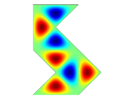
Figure 22: (Color online) First triangular mode (ninth mode).

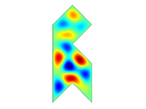
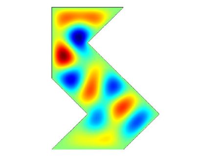
Figure 23: (Color online) $15$th mode.

A.2 The $17$ families of isospectral pairs and their mathematical construction

The following gallery presents the $17$ known families of isospectral pairs, as obtained by Buser et al. (1994); Okada and Shudo (2001); Giraud (2005b). All are based on a Sunada triple $(G,G_{1},G_{2})$, where $G=\mathbf{PSL}(n+1,q)$ is the special linear automorphism group of a finite projective space of $(q^{n+1}-1)/(q-1)$ points, and $G_{1},G_{2}$ are two subgroups, generated by $a_{1},b_{1},c_{1}$ and $a_{2},b_{2},c_{2}$ given below, respectively. These automorphisms are collineations of order 2 of the underlying finite projective space; $a_{1},b_{1},c_{1}$ act on points while $a_{2},b_{2},c_{2}$ act on hyperplanes, numbered from $0$ to $(q^{n+1}-1)/(q-1)-1$. The generators $a_{i}$ and $b_{i}$ allow to construct the graphs (see section II.1) that specify the way in which the tiles are glued together. Figures 24 to 40 give examples of pairs of isospectral billiards obtained by applying the unfolding rules on an equilateral triangle (left panel) or on a scalene triangle (right panel).

Interestingly, the structure of pairs $13_{6}$ and $15_{2}$ forbids the construction of any proper billiard, that is, structures where triangles do not overlap. It is quite simple to convince oneself of this fact. In the case of the billiard $13_{6}$ (see Fig. 32), the initial triangle is unfolded six times around each of its corner. Clearly, to have a non-overlapping billiard, each angle should be less than $\pi/3$, which is impossible unless the initial triangle is equilateral.

For the billiard $15_{2}$ (see Fig. 37), the initial triangle is unfolded six times around two of its corners, four times around the third one, and thus two angles have to be less than $\pi/3$ and one less than $\pi/2$. While it is possible to construct such a billiard, it is impossible to get a pair of planar billiards. Indeed, the role of the angles is exchanged from one billiard to the other, which leads to the condition that the three angles be less than $\pi/3$. On the other hand, the presence of a loop in the pair $21_{1}$ requires that one angle of the base triangle be $\pi/3$.

Figure 24: Pair $7_{1}$. Sunada triple $G=\mathbf{PSL}(3,2)$, $G_{i}=\langle a_{i},b_{i},c_{i}\rangle$, $i=1,2$, with $a_{1}=(0\ 1)(2\ 5)$, $b_{1}=(0\ 2)(3\ 4)$, $c_{1}=(0\ 4)(1\ 6)$, $a_{2}=(0\ 4)(2\ 3)$, $b_{2}=(0\ 1)(4\ 6)$, $c_{2}=(0\ 2)(1\ 5)$.

Figure 25: Pair $7_{2}$. Sunada triple $G=\mathbf{PSL}(3,2)$, $G_{i}=\langle a_{i},b_{i},c_{i}\rangle$, $i=1,2$, with $a_{1}=(0\ 1)(2\ 5)$, $b_{1}=(1\ 5)(3\ 4)$, $c_{1}=(0\ 4)(1\ 6)$, $a_{2}=(0\ 4)(2\ 3)$, $b_{2}=(0\ 6)(1\ 4)$, $c_{2}=(0\ 2)(1\ 5)$.

Figure 26: Pair $7_{3}$. Sunada triple $G=\mathbf{PSL}(3,2)$, $G_{i}=\langle a_{i},b_{i},c_{i}\rangle$, $i=1,2$, with $a_{1}=(2\ 5)(4\ 6)$, $b_{1}=(1\ 5)(3\ 4)$, $c_{1}=(0\ 4)(1\ 6)$, $a_{2}=(0\ 3)(2\ 4)$, $b_{2}=(0\ 6)(1\ 4)$, $c_{2}=(0\ 2)(1\ 5)$.

Figure 27: Pair $13_{1}$. Sunada triple $G=\mathbf{PSL}(3,3)$, $G_{i}=\langle a_{i},b_{i},c_{i}\rangle$, $i=1,2$, with $a_{1}=(0\ 12)(1\ 10)(3\ 5)(6\ 7)$, $b_{1}=(0\ 10)(2\ 9)(3\ 4)(5\ 8)$, $c_{1}=(0\ 4)(1\ 6)(2\ 11)(9\ 12)$, $a_{2}=(0\ 4)(2\ 3)(6\ 8)(9\ 10)$, $b_{2}=(0\ 12)(1\ 4)(5\ 11)(6\ 9)$, $c_{2}=(0\ 10)(1\ 5)(2\ 7)(3\ 12)$.

Figure 28: Pair $13_{2}$. Sunada triple $G=\mathbf{PSL}(3,3)$, $G_{i}=\langle a_{i},b_{i},c_{i}\rangle$, $i=1,2$, with $a_{1}=(0\ 12)(1\ 10)(3\ 5)(6\ 7)$, $b_{1}=(1\ 12)(2\ 9)(3\ 8)(4\ 5)$, $c_{1}=(0\ 4)(1\ 6)(2\ 11)(9\ 12)$, $a_{2}=(0\ 4)(2\ 3)(6\ 8)(9\ 10)$, $b_{2}=(0\ 1)(4\ 12)(5\ 11)(8\ 10)$, $c_{2}=(0\ 10)(1\ 5)(2\ 7)(3\ 12)$.

Figure 29: Pair $13_{3}$. Sunada triple $G=\mathbf{PSL}(3,3)$, $G_{i}=\langle a_{i},b_{i},c_{i}\rangle$, $i=1,2$, with $a_{1}=(1\ 7)(3\ 5)(4\ 9)(6\ 10)$, $b_{1}=(1\ 12)(2\ 9)(3\ 8)(4\ 5)$, $c_{1}=(0\ 4)(1\ 6)(2\ 11)(9\ 12)$, $a_{2}=(0\ 9)(4\ 10)(6\ 8)(7\ 12)$, $b_{2}=(0\ 1)(4\ 12)(5\ 11)(8\ 10)$, $c_{2}=(0\ 10)(1\ 5)(2\ 7)(3\ 12)$.

Figure 30: Pair $13_{4}$. Sunada triple $G=\mathbf{PSL}(3,3)$, $G_{i}=\langle a_{i},b_{i},c_{i}\rangle$, $i=1,2$, with $a_{1}=(1\ 7)(3\ 5)(4\ 9)(6\ 10)$, $b_{1}=(0\ 5)(1\ 2)(6\ 12)(9\ 11)$, $c_{1}=(0\ 4)(1\ 6)(2\ 11)(9\ 12)$, $a_{2}=(0\ 9)(4\ 10)(6\ 8)(7\ 12)$, $b_{2}=(0\ 11)(1\ 8)(2\ 7)(3\ 4)$, $c_{2}=(0\ 10)(1\ 5)(2\ 7)(3\ 12)$.

Figure 31: Pair $13_{5}$. Sunada triple $G=\mathbf{PSL}(3,3)$, $G_{i}=\langle a_{i},b_{i},c_{i}\rangle$, $i=1,2$, with $a_{1}=(1\ 7)(3\ 5)(4\ 9)(6\ 10)$, $b_{1}=(0\ 5)(1\ 2)(6\ 12)(9\ 11)$, $c_{1}=(0\ 4)(1\ 6)(2\ 11)(9\ 12)$, $a_{2}=(0\ 9)(4\ 10)(6\ 8)(7\ 12)$, $b_{2}=(0\ 11)(1\ 8)(2\ 7)(3\ 4)$, $c_{2}=(0\ 10)(1\ 5)(2\ 7)(3\ 12)$.

Figure 32: Pair $13_{6}$. Sunada triple $G=\mathbf{PSL}(3,3)$, $G_{i}=\langle a_{i},b_{i},c_{i}\rangle$, $i=1,2$, with $a_{1}=(0\ 2)(1\ 7)(3\ 6)(5\ 10)$, $b_{1}=(0\ 6)(2\ 4)(3\ 8)(5\ 9)$, $c_{1}=(0\ 5)(1\ 2)(6\ 12)(9\ 11)$, $a_{2}=(0\ 7)(3\ 11)(6\ 8)(9\ 12)$, $b_{2}=(0\ 8)(1\ 10)(5\ 11)(7\ 9)$, $c_{2}=(0\ 11)(1\ 8)(2\ 7)(3\ 4)$.

Figure 33: Pair $13_{7}$. Sunada triple $G=\mathbf{PSL}(3,3)$, $G_{i}=\langle a_{i},b_{i},c_{i}\rangle$, $i=1,2$, with $a_{1}=(0\ 2)(1\ 7)(3\ 6)(5\ 10)$, $b_{1}=(0\ 4)(2\ 3)(6\ 8)(9\ 10)$, $c_{1}=(0\ 5)(1\ 2)(6\ 12)(9\ 11)$, $a_{2}=(0\ 7)(3\ 11)(6\ 8)(9\ 12)$, $b_{2}=(0\ 12)(1\ 10)(3\ 5)(6\ 7)$, $c_{2}=(0\ 11)(1\ 8)(2\ 7)(3\ 4)$.

Figure 34: Pair $13_{8}$. Sunada triple $G=\mathbf{PSL}(3,3)$, $G_{i}=\langle a_{i},b_{i},c_{i}\rangle$, $i=1,2$, with $a_{1}=(0\ 10)(1\ 5)(2\ 7)(3\ 12)$, $b_{1}=(0\ 4)(2\ 3)(6\ 8)(9\ 10)$, $c_{1}=(0\ 5)(1\ 2)(6\ 12)(9\ 11)$, $a_{2}=(0\ 4)(1\ 6)(2\ 11)(9\ 12)$, $b_{2}=(0\ 12)(1\ 10)(3\ 5)(6\ 7)$, $c_{2}=(0\ 11)(1\ 8)(2\ 7)(3\ 4)$.

Figure 35: Pair $13_{9}$. Sunada triple $G=\mathbf{PSL}(3,3)$, $G_{i}=\langle a_{i},b_{i},c_{i}\rangle$, $i=1,2$, with $a_{1}=(0\ 10)(1\ 5)(2\ 7)(3\ 12)$, $b_{1}=(1\ 10)(3\ 6)(5\ 7)(9\ 11)$, $c_{1}=(0\ 5)(1\ 2)(6\ 12)(9\ 11)$, $a_{2}=(0\ 4)(1\ 6)(2\ 11)(9\ 12)$, $b_{2}=(0\ 3)(2\ 4)(6\ 8)(7\ 11)$, $c_{2}=(0\ 11)(1\ 8)(2\ 7)(3\ 4)$.

Figure 36: Pair $15_{1}$. Sunada triple $G=\mathbf{PSL}(4,2)$, $G_{i}=\langle a_{i},b_{i},c_{i}\rangle$, $i=1,2$, with $a_{1}=(0\ 14)(1\ 12)(2\ 6)(4\ 5)(7\ 11)(9\ 10)$, $b_{1}=(1\ 13)(2\ 7)(4\ 6)(8\ 9)$, $c_{1}=(1\ 14)(2\ 12)(3\ 4)(8\ 11)$, $a_{2}=(0\ 11)(1\ 5)(3\ 4)(6\ 10)(8\ 9)(13\ 14)$, $b_{2}=(0\ 10)(1\ 2)(6\ 9)(12\ 14)$, $c_{2}=(0\ 5)(2\ 4)(6\ 7)(11\ 14)$.

Figure 37: Pair $15_{2}$. Sunada triple $G=\mathbf{PSL}(4,2)$, $G_{i}=\langle a_{i},b_{i},c_{i}\rangle$, $i=1,2$, with $a_{1}=(0\ 14)(1\ 12)(2\ 6)(4\ 5)(7\ 11)(9\ 10)$, $b_{1}=(1\ 13)(2\ 7)(4\ 6)(8\ 9)$, $c_{1}=(0\ 12)(1\ 6)(3\ 5)(7\ 8)$, $a_{2}=(0\ 11)(1\ 5)(3\ 4)(6\ 10)(8\ 9)(13\ 14)$, $b_{2}=(0\ 10)(1\ 2)(6\ 9)(12\ 14)$, $c_{2}=(0\ 13)(1\ 11)(2\ 3)(7\ 10)$.

Figure 38: Pair $15_{3}$. Sunada triple $G=\mathbf{PSL}(4,2)$, $G_{i}=\langle a_{i},b_{i},c_{i}\rangle$, $i=1,2$, with $a_{1}=(0\ 14)(2\ 11)(4\ 7)(5\ 6)(8\ 10)(12\ 13)$, $b_{1}=(1\ 13)(2\ 7)(4\ 6)(8\ 9)$, $c_{1}=(0\ 12)(1\ 6)(3\ 5)(7\ 8)$, $a_{2}=(0\ 9)(2\ 5)(3\ 4)(6\ 8)(10\ 11)(12\ 13)$, $b_{2}=(0\ 10)(1\ 2)(6\ 9)(12\ 14)$, $c_{2}=(0\ 13)(1\ 11)(2\ 3)(7\ 10)$.

Figure 39: Pair $15_{4}$. Sunada triple $G=\mathbf{PSL}(4,2)$, $G_{i}=\langle a_{i},b_{i},c_{i}\rangle$, $i=1,2$, with $a_{1}=(0\ 14)(2\ 11)(4\ 7)(5\ 6)(8\ 10)(12\ 13)$, $b_{1}=(1\ 4)(2\ 8)(7\ 9)(8\ 9)$, $c_{1}=(0\ 12)(1\ 6)(3\ 5)(7\ 8)$, $a_{2}=(0\ 9)(2\ 5)(3\ 4)(6\ 8)(10\ 11)(12\ 13)$, $b_{2}=(6\ 9)(7\ 13)(12\ 14)$, $c_{2}=(0\ 13)(1\ 11)(2\ 3)(7\ 10)$.

Figure 40: Pair $21_{1}$. Sunada triple $G=\mathbf{PSL}(3,4)$, $G_{i}=\langle a_{i},b_{i},c_{i}\rangle$, $i=1,2$, with $a_{1}=(2\ 7)(3\ 11)(5\ 12)(8\ 18)(13\ 14)(15\ 17)(16\ 20)$, $b_{1}=(0\ 17)(3\ 8)(4\ 12)(6\ 13)(9\ 19)(14\ 15)(16\ 18)$, $c_{1}=(1\ 8)(2\ 16)(4\ 11)(5\ 19)(7\ 14)(10\ 17)(13\ 20)$, $a_{2}=(0\ 1)(4\ 17)(7\ 12)(9\ 16)(10\ 20)(11\ 13)(15\ 19)$, $b_{2}=(0\ 20)(3\ 16)(6\ 11)(8\ 15)(9\ 19)(10\ 12)(14\ 18)$, $c_{2}=(1\ 8)(2\ 16)(4\ 11)(5\ 19)(7\ 14)(10\ 17)(13\ 20)$.

Appendix B Spectral problems for Lie geometries

B.1 Generalized polygons

Generalized polygons were introduced by Tits (1959) in order to have a geometric interpretation of certain Chevalley groups of rank $2$. They are also the building bricks of (Tits) buildings, the natural geometries for the groups with a BN-pair.

A group $G$ is said to have a BN-pair $(B,N)$, where $B,N$ are subgroups of $G$, if the following properties are satisfied: (BN1) $\langle B,N\rangle=G$; (BN2) $H=B\cap N\unlhd N$ and $N/H=W$ is a Coxeter group (see, e.g., Tits (1974)) with distinct generators $s_{1},s_{2},\ldots,s_{n}$; (BN3) $Bs_{i}BwB\subseteq BwB\cup Bs_{i}wB$ whenever $w\in W$ and $i\in\{1,2,\ldots,n\}$; (BN4) $s_{i}Bs_{i}\neq B$ for all $i\in\{1,2,\ldots,n\}$. The subgroup $B$, respectively $W$, is a Borel subgroup, respectively the Weyl group, of $G$. The natural number $n$ is called the rank of the BN-pair.

Example. Suppose $\mathbf{PG}(1,q)$ is the projective line over the finite field $\mathbb{F}_{q}$; so $\mathbf{PG}(1,q)$ has $q+1$ points. Consider the natural action of $\mathbf{PSL}(2,q)$ on $\mathbf{PG}(1,q)$, and let $x$ and $y$ be distinct points of the projective line. Set $B=\mathbf{PSL}(2,q)_{x}$ and $N=\mathbf{PSL}(2,q)_{\{x,y\}}$. Then $(B,N)$ is a BN-pair for $\mathbf{PSL}(2,q)$. Here $N/(B\cap N)=W$ is just the group of order $2$.

Example. Consider the Desarguesian projective plane $\mathbf{PG}(2,q)$, and $\mathbf{PSL}(3,q)$ in its natural action on the latter plane. Let $(x,L)$ be an incident point-line pair, and $\Delta$ a triangle (in the ordinary sense) that contains $x$ as a point and $L$ as a side. Set $B=\mathbf{PSL}(3,q)_{(x,L)}$ and $N=\mathbf{PSL}(3,q)_{\Delta}$; then $(B,N)$ is a BN-pair for $\mathbf{PSL}(3,q)$ and $N/(B\cap N)=W$ is the dihedral group of order $6$.

See Payne and Thas (1984); Van Maldeghem (1998); Thas et al. (2006); Thas (2004) for standard references on the subject of generalized polygons. In this paper we consider only thick GPs.

Now let $G$ be a group with a BN-pair $(B,N)$ of rank $2$. One can associate a generalized polygon $\mathcal{B}(G)$ with the group $G$ in the following way. For this purpose, define $P_{1}=\langle B,B^{s_{1}}\rangle$ and $P_{2}=\langle B,B^{s_{2}}\rangle$.

• Call the right cosets of $P_{1}$ “points”.

• Call the right cosets of $P_{2}$ “lines”.

• Call two such (distinct) cosets “incident” if their intersection is nonempty (so $P_{1}g$ is incident with $P_{2}h$, $g,h\in G$, if $P_{1}g\cap P_{2}h\neq\emptyset$).

Then $\mathcal{B}(G)$ is a GP — say a generalized $n$-gon for some natural number $n$ — on which $G$ acts naturally as an automorphism group that permutes transitively the ordered $n$-gons (in the ordinary sense).

Conjecture [J. Tits, (Tits, 1974, §11.5.1)]. If a finite thick generalized $n$-gon is such that the automorphism group permutes transitively the ordered $n$-gons (that is, if $\Delta$ is associated with a BN-pair), then $\Delta$ is isomorphic with the GP of an absolutely simple group over a finite field, or with the GP of a Ree group of type ${}^{2}\mathbf{F}_{4}$ over a finite field.

For more on the classification of BN-pairs of rank $2$, see Thas (2009, 2010) and Thas and Van Maldeghem (2008).

B.2 Duality principle

Let $\Gamma=(\mathcal{P},\mathcal{B},\mathbf{I})$ be a GP of order $(s,t)$. Then $\Gamma^{D}=(\mathcal{B},\mathcal{P},\mathbf{I})$ clearly again is a GP, but now of order $(t,s)$. (The latter geometry is called the point-line dual of $\Gamma$.) So any theorem which holds for a GP, has a dual interpretation; we call this principle “duality principle”.

B.3 Automorphisms and isomorphisms

Let $\Gamma=(\mathcal{P},\mathcal{B},\mathbf{I})$ and $\Gamma^{\prime}=(\mathcal{P}^{\prime},\mathcal{B}^{\prime},\mathbf{I}^{\prime})$ be GPs. Then an isomorphism between $\Gamma$ and $\Gamma^{\prime}$ is a pair $(\alpha,\beta)$ for which $\alpha$ is a bijection between $\mathcal{P}$ and $\mathcal{P}^{\prime}$, $\beta$ is a bijection between $\mathcal{B}$ and $\mathcal{B}^{\prime}$, and $x\mathbf{I}L$ (in $\Gamma$) if and only if $x^{\alpha}\mathbf{I}L^{\beta}$. If there is an isomorphism between $\Gamma$ and $\Gamma^{\prime}$, we say they are “isomorphic”, and write $\Gamma\cong\Gamma^{\prime}$.

If $\Gamma=\Gamma^{\prime}$ one speaks of an “automorphism”. The set of all automorphisms of a GP forms a group, and the classical examples of GPs are those examples that are associated with a Chevalley group (or, equivalently, with a “classical” BN-pair), cf. Van Maldeghem (1998) for more details.

B.4 Point spectra and order

Let $\Gamma$ be a finite thick GP of order $(s,t)$, with associated collinearity matrix $\mathbf{A}$. Our first concern is to calculate $\mathrm{spec}(\mathbf{A})$.

First, we recall the theorem of Feit and Higman (1964): A finite thick generalized $n$-gon exists if and only if $n\in\{3,4,6,8\}$. We will do a case-by-case analysis according to this result.

Case $n=3$.

Recall that a generalized $3$-gon is the same as an axiomatic projective plane. Now let $\Gamma$ be a finite projective plane of order $n$, $n\geq 2$, and put $n^{2}+n+1=\mathfrak{v}$, its number of points. Then $\mathbf{A}=\mathbb{J}_{\mathfrak{v}}-\mathbb{I}_{\mathfrak{v}}$, where $\mathbb{J}_{\mathfrak{v}}$ is the all $1$ $\mathfrak{v}\times\mathfrak{v}$-matrix, and $\mathbb{I}_{\mathfrak{v}}$ the $\mathfrak{v}\times\mathfrak{v}$-identity matrix. It follows that

$$\mathrm{spec}(\mathbf{A})=\{-1,\mathfrak{v}-1\}.$$ (148)

So if the spectra of two finite projective planes coincide, their orders do as well.

Case $n=4$.

Let $\Gamma$ be a thick generalized $4$-gon, or also ”generalized quadrangle” (GQ) of order $(s,t)$. Then using the results of Payne and Thas (1984, 1.2.2), we have

$$\mathrm{spec}(\mathbf{A})=\{-t-1,s-1,s(t+1)\}.$$ (149)

Now let $\Gamma^{\prime}$ also be a thick GQ, with the same spectrum, of order $(s^{\prime},t^{\prime})$. There is only one negative eigenvalue, so $-t-1=-t^{\prime}-1$ and $t=t^{\prime}$. Since $s-1<s(t+1)$ ($s^{\prime}-1<s^{\prime}(t^{\prime}+1)$), it also follows that $s=s^{\prime}$, and hence $\Gamma$ and $\Gamma^{\prime}$ have the same order.

Case $n=6$.

For this case, we need one more definition. A distance regular graph $G$ with diameter $d$ is a regular connected graph with valency $k$ for which there exist natural numbers $b_{0}=k,b_{1},\ldots,b_{d-1};c_{1}=1,c_{2},\ldots,c_{d}$ such that for each pair of vertices $x$ and $y$ at distance $j$, we have

• $|\Gamma_{j-1}(y)\cap\Gamma_{1}(x)|=c_{j}$, $1\leq j\leq d$;

• $|\Gamma_{j+1}(y)\cap\Gamma_{1}(x)|=b_{j}$, $0\leq j\leq d-1$.

Now define the constants $a_{j}=|\Gamma_{j}(y)\cap\Gamma_{1}(x)|$ for $0\leq j\leq d$. A result of Brouwer et al. (1989) claims that the eigenvalues of the point graph of $G$ are the eigenvalues of the following ”intersection matrix”:

$$\left(\begin{array}[]{ccccc}0&1&&&\\ k&a_{1}&c_{2}&&\\ &b_{1}&a_{2}&\cdots&\\ &\vdots&b_{2}&\cdots&\\ &&\vdots&&c_{d}\\ &&&b_{d-1}&a_{d}\\ \end{array}\right).\\$$ (150)

It just so happens to be that the collinearity graph of a generalized hexagon (a generalized $6$-gon) is distance regular with a diameter of $3$. An easy exercise yields, for a thick generalized hexagon of order $(s,t)$, the following intersection matrix:

$$\mathbf{B}=\left(\begin{array}[]{cccc}0&1&0&0\\ s(t+1)&s-1&1&0\\ 0&st&s-1&t+1\\ 0&0&st&(t+1)(s-1)\end{array}\right).$$ (151)

The determinant of $\mathbf{B}-x\mathbb{I}_{4}$ has the following roots:

$$x=-t-1,\ \ x=s(t+1),\ \ x=s-1-\sqrt{st},\ \ x=s-1+\sqrt{st}.$$ (152)

One observes that $-t-1$ is strictly the smallest eigenvalue, while $s(t+1)$ is the largest. It now easily follows that if a generalized hexagon of order $(s^{\prime},t^{\prime})$ has the same spectrum as $\Gamma$, then it has the same order.

Case $n=8$. Let $\Gamma$ be a thick generalized octagon ($8$-gon) of order $(s,t)$. Again, the point graph is distance regular, now with a diameter of $4$. The intersection matrix is easily seen to be the following:

$$\mathbf{B}=\left(\begin{array}[]{ccccc}0&1&0&0&0\\ s(t+1)&s-1&1&0&0\\ 0&st&s-1&1&0\\ 0&0&st&s-1&t+1\\ 0&0&0&st&(t+1)(s-1)\end{array}\right),$$ (153)

which has eigenvalues

$$x=-t-1,\ \ x=s-1,\ \ x=s(t+1),$$

$$x=s-1-\sqrt{2st},\ \ x=s-1+\sqrt{2st}.$$ (154)

The third largest eigenvalue is $s-1$, so if $\Gamma^{\prime}$ is a thick generalized octagon of order $(s^{\prime},t^{\prime})$ with the same spectrum, then $s=s^{\prime}$. As $s(t+1)$ is the largest eigenvalue of $\mathrm{spec}(\mathbf{A})$, it follows that $t=t^{\prime}$. This ends the proof of Theorem VIII.2.$\blacksquare$

B.5 Concluding remarks

In this section, we make some comments on generalized polygons that are characterized by their order.

Projective planes. For some small values, e.g. $n=2$, it is known that there is a unique projective plane of order $n$ (up to isomorphism). It is well-known, however, that as soon as $n$ is large enough and not a prime, nonisomorphic examples exist. On the other hand, for $p$ a prime, only one example is known, namely the classical example $\mathbf{PG}(2,p)$ arising from a BN-pair in $\mathbf{PSL}(2,p)$.

Generalized quadrangles. Many infinite classes of GQs are known, and several examples with small parameters are completely determined by their order. We refer the interested reader to (Payne and Thas, 1984, Chapter 6) for these examples. We make some comments according to the known orders. Below, $q$ is always a prime power. We also assume $s\leq t$ by reasons of duality. [Details and references can be found in (Thas, 2004, Chapter 3).]

• $(s,t)=(q^{2},q^{3})$. Only one example is known (for each $q$), namely, the Hermitian quadrangle $\mathbf{H}(4,q^{2})$.

• $(s,t)=(q-1,q+1)$. If $q\geq 8$ and $q$ is even, nonisomorphic examples are known for every $q$. In the other cases, only unique examples are known.

• $(s,t)=(q,q)$. If $q$ is odd, nonisomorphic examples are known for every $q$. If $q\geq 8$ and $q$ is even, we have the same remark. The other values give unique examples.

• $(s,t)=(q,q^{2})$. If $q\geq 5$, nonisomorphic examples are known for every $q$. The examples of order $(2,4)$ and $(3,9)$ are unique.

Generalized hexagons. Up to duality, only two classes of generalized hexagons are known (both associated with classical groups): the split Cayley hexagons $\mathbf{H}(q)$ of order $q$, $q$ a prime power, and the twisted triality hexagons $\mathbf{T}(q,q^{3})$ of order $(q,q^{3})$, cf. (Van Maldeghem, 1998, Chapter 2). We know that $\mathbf{H}(q)\cong\mathbf{H}(q)^{D}$ if and only if $q$ is a power of $3$ Van Maldeghem (1998). If $q$ is not a power of $3$, $\mathbf{H}(q)\not\cong\mathbf{H}(q)^{D}$, while both have the same spectrum.

Generalized octagons. Up to duality, the only known thick finite generalized octagons are the Ree-Tits octagons $\mathbf{O}(q)$, where $q$ is an odd power of $2$; they can be constructed from a BN-pair in the Ree groups of type ${}^{2}\mathbf{F}_{4}$ (Van Maldeghem, 1998, Chapter 2). They have order $(q,q^{2})$.

Finally, see the monograph Cvetkovic et al. (1998) for more information on graph spectra. van Dam and Haemers (2003) surveyed the known cases of graphs that are determined by their spectrum. Some generalized quadrangles with small parameters are mentioned that are uniquely determined by their spectrum. Since such examples must have the property that they are determined by their order, Payne and Thas (1984, Chapter 6) also yielded these examples.

Appendix C Livsic cohomology

In this appendix we describe a connection between isospectrality and cohomology. Let $(M,g)$ be a Riemannian manifold without boundaries. The length spectrum is the discrete set

$$Lsp(M,g)=\{L_{\gamma_{1}}<L_{\gamma_{2}}<\cdots\}$$ (155)

of lengths of closed geodesics $\gamma_{j}$.

Denote by $(T^{*}M,\sum_{j}dx_{j}\wedge d\xi_{j})$ the cotangent bundle of $M$ equipped with its natural symplectic form. Given the metric $g$, we define the metric Hamiltonian by

$$H(x,\xi)=|\xi|=\sqrt{\sum_{ij=1}^{n+1}g^{ij}(x)\xi_{i}\xi_{j}},$$ (156)

and define the energy surface to be the unit sphere bundle

$$S^{*}M=\{(x,\xi)\parallel|\xi|=1\}.$$ (157)

The geodesic flow $G^{t}$ is the Hamiltonian flow

$$G^{t}=\mbox{exp}t\Xi_{H}:T^{*}M\setminus 0\mapsto T^{*}M\setminus 0,$$ (158)

where $\Xi_{H}$ is the Hamiltonian vector field. Since it is homogeneous of degree $1$ with respect to the dilatation $(x,\xi)\mapsto(x,r\xi)$, $r>0$, one can restrict $G^{t}$ to $S^{*}M$. Its generator is also denoted by $\Xi$.

Livsic’s cohomological problem asks whether a cocycle $f\in C^{\infty}(S^{*}M)$ satisfying

$$\int_{\lambda}fds=0$$ (159)

for every closed geodesic of the metric $g$ is necessarily a coboundary $f=\Xi(g)$, where $\Xi$ is the generator of the geodesic flow $G^{t}$ and $g$ is a function with a certain degree of regularity. Under a deformation $g_{\epsilon}$ of a metric $g=g_{0}$ preserving the extended $Lsp(M,g)$ (including multiplicities), one has

$$\int_{\lambda}\dot{g}ds=0,\ \ \forall\lambda.$$ (160)

When the cohomology is trivial, one can therefore write $\dot{g}=\Xi(f)$ for some $f$ with the given regularity. One does not expect the cohomology to be trivial in general settings, but the results might be interesting for the length spectral deformation problem.

References

- Aurich et al. (1997) Aurich, R., A. Bäcker, and F. Steiner, 1997, Int. J. Mod. Phys. B 11, 805.
- Aurich and Steiner (1990) Aurich, R., and F. Steiner, 1990, Physica D 43, 155.
- Balian and Bloch (1974) Balian, R., and C. Bloch, 1974, Ann. Phys. (N. Y. ) 85, 514.
- Baltes and Hilf (1976) Baltes, H., and E. R. Hilf, 1976, Spectra of Finite Systems (Bibliographisches Institut, Mannheim).
- Bérard (1989) Bérard, P., 1989, Astérisque 177-178, 127.
- Bérard (1992) Bérard, P., 1992, Math. Ann. 292, 547.
- Bérard (1993) Bérard, P., 1993, J. London Math. Soc. 48, 565.
- Bérard and Besson (1980) Bérard, P., and G. Besson, 1980, Ann. Inst. Fourier, Grenoble 30, 237.
- Berry (1981) Berry, M. V., 1981, Eur. J. Phys. 2, 91.
- Berry and Tabor (1976) Berry, M. V., and M. Tabor, 1976, Proc. Roy. Soc. London 349, 101.
- Berry and Tabor (1977) Berry, M. V., and M. Tabor, 1977, Proc. Roy. Soc. London 356, 375.
- Berry and Wilkinson (1984) Berry, M. V., and M. Wilkinson, 1984, Proc. R. Soc. London 392, 15.
- Betcke and Trefethen (2005) Betcke, T., and L. N. Trefethen, 2005, SIAM Review 47(3), 469.
- Blum et al. (2002) Blum, G., S. Gnutzmann, and U. Smilansky, 2002, Phys. Rev. Lett. 88, 114101.
- Bohigas et al. (1984) Bohigas, O., M.-J. Giannoni, and C. Schmit, 1984, Phys. Rev. Lett. 52, 1.
- Brooks (1988) Brooks, R., 1988, Amer. Math. Monthly 95, 823.
- Brouwer et al. (1989) Brouwer, A. E., A. M. Cohen, and A. Neumaier, 1989, Distance-Regular Graphs (Springer, Heidelberg).
- Bruening et al. (2008) Bruening, J., D. Klawonn, and C. Puhle, 2008, J. Phys. A: Math. Theor. 40, 15143.
- Buser (1988) Buser, P., 1988, Geometry and Analysis on Manifolds (Katata/Kyoto, 1987), Lecture Notes in Math. 1339, Springer, Berlin , 64.
- Buser et al. (1994) Buser, P., J. Conway, and P. Doyle, 1994, Int. Math. Res. Notices 9, 391.
- Chang and Deturck (1989) Chang, P.-K., and D. Deturck, 1989, Proc. Amer. Math. Soc. 105(4), 1033.
- Chapman (1995) Chapman, S. J., 1995, Am. Math. Monthly 102(2), 124.
- Chladni (1802) Chladni, E. (ed.), 1802, Die Akustik (Breitkopf und Härtel, Leipzig).
- Conway et al. (1985) Conway, J. H., and R. T. Curtis, and S. P. Norton, and R. A. Parker, and R. A. Wilson 1985, Atlas of Finite Groups: Maximal Subgroups and Ordinary Characters for Simple Groups (Oxford University Press, Oxford).
- Conway and Sloane (1992) Conway, J. H., and N. J. A. Sloane, 1992, Int. Math. Res. Notices 1992, 93.
- Courant and Hilbert (1953) Courant, R., and D. Hilbert, 1953, Methods of Mathematical Physics, volume I (Interscience, New York).
- Cvetkovic et al. (1998) Cvetkovic, D. M., M. Doob, and H. Sachs, 1998, Spectra of Graphs: Theory and Applications, 3rd ed. (Wiley, New York)
- Descloux and Tolley (1983) Descloux, J., and M. Tolley, 1983, Comput. Methods Appl. Mech. Engrg. 39, 37.
- Dhar et al. (2003) Dhar, A., D.M. Rao, N. UdayaShankar, and S. Sridhar, 2003, Phys. Rev. E 68, 026208.
- Doyle and Rossetti (2004) Doyle, P. G. and Rossetti, J. P., 2004, Geom. Topol. 8, 1227.
- Driscoll (1997) Driscoll, T. A., 1997, SIAM Rev. 39(1), 1.
- Driscoll and Gottlieb (2003) Driscoll, T. A., and H. P. W. Gottlieb, 2003, Phys. Rev. E 68, 016702.
- Earnest and Nipp (1991) Earnest, A. G., and G. Nipp, 1991, C. R. Math. Acad. Sci. Can. 13, 33.
- Even and Pieranski (1999) Even, C., and P. Pieranski, 1999, Europhys. Lett. 47, 531.
- Feit and Higman (1964) Feit, W., and D. Higman, 1964, J. Algebra 1, 114.
- Feynman and Hibbs (1965) Feynman, R. P. and Hibbs, A. R., 1965, Quantum Mechanics and Path Integrals (Mc. Graw-Hill, New York).
- Fox et al. (1967) Fox, L., P. Henrici, and C. Moler, 1967, SIAM J. Numer. Anal. 4, 89.
- Fulling and Kuchment (2005) Fulling, S. A., and P. Kuchment, 2005, Inverse Problems 21, 1391.
- Garabedian (1998) Garabedian, P. R., 1998, Partial Differential Equations (AMS Chelsea Publ., Amer. Math. Soc., Providence, RI).
- Garabedian and Schiffer (1952) Garabedian, P. R., and M. Schiffer, 1952, J. d’Anal. Math. 2, 281.
- Gassmann (1926) Gassmann, F., 1926, Math. Z. 25, 665.
- Georgeot and Prange (1995) Georgeot, B., and R. E. Prange, 1995, Phys. Rev. Lett. 74(15), 2851.
- Gerst (1970) Gerst, I., 1970, Acta Arith. 27, 121.
- Giraud (2004) Giraud, O., 2004, J. Phys. A: Math. Gen. 37(7), 2751.
- Giraud (2005a) Giraud, O., 2005a, J. Phys. A 38, L477.
- Giraud (2005b) Giraud, O., 2005b, J. Phys. A: Math. Gen. 38, L477.
- Gnutzmann et al. (2005) Gnutzmann, S., U. Smilansky, and N. Sondergaard, 2005, J. Phys. A: Math. Gen. 38, 8921.
- Gordon et al. (1992a) Gordon, C., D. Webb, and S. Wolpert, 1992a, Invent. math. 110, 1.
- Gordon et al. (1992b) Gordon, C., D. Webb, and S. Wolpert, 1992b, Bull. Amer. Math. Soc. 27, 134.
- Gordon (1986) Gordon, C. S., 1986, Contemp. Math. 51, 63.
- Gordon and Webb (1994) Gordon, C. S., and D. L. Webb, 1994, Proc. Amer. Math. Soc. 120, 981.
- Gorenstein (1980) Gorenstein, D., 1980, Finite Groups. Second edition (Chelsea Publishing Co., New York).
- Gottlieb (2004) Gottlieb, H. P. W., 2004, Inverse problems 20, 155.
- Gottlieb and McManus (1998) Gottlieb, H. P. W., and J. P. McManus, 1998, Journal of Sound and Vibration 212(2), 253.
- Guhr et al. (1998) Guhr, T., A. Müller-Groeling, and H. Weidenmüller, 1998, Phys. Rep. 299, 189.
- Gutkin and Judge (2000) Gutkin, E., and C. Judge, 2000, Duke Math. J. 103(2), 191.
- Gutkin and Smilansky (2001) Gutkin, B., and U. Smilansky, 2001, J. Phys. A 34(31), 6061.
- Gutzwiller (1991) Gutzwiller, M. C., 1991, in Chaos and Quantum Mechanics, edited by M.-J. Giannoni, A. Voros, and J. Zinn-Justin (North Holland, Amsterdam), les Houches Summer School Lectures, Session LII, 1989.
- Hannay and Thain (2003) Hannay, J. H., and A. Thain, 2003, J. Phys. A: Math. Gen. 36, 4063.
- Hezari and Zelditch (2009) Hezari, H., S. Zelditch, 2009, Geom. Funct. Anal. 20, 160.
- Hirschfeld (1998) Hirschfeld, J. W. P., 1998, Projective Geometries over Finite Fields. Second edition (The Clarendon Press, Oxford University Press, New York).
- Hughes and Piper (1973) Hughes, D. R., and F. C. Piper, 1973, Projective Planes (Springer-Verlag, New York/Heidelberg/Berlin).
- Iantchenko et al. (2002) Iantchenko, A., J. Sjöstrand, and M. Zworski, 2002, Math. Res. Lett. 9, 337.
- Ikeda (1980) Ikeda, A., 1980, Ann. Sci. Ecole Normale Super. 13, 303.
- Ivanov et al. (1977) Ivanov, L., L. Kotko, and S. Krein, 1977, Boundary Value Problems in Variable Domains, volume 19 (Math. Inst. of Lithuanian Acad. Sci., Vilnius).
- Jakobson et al. (2006) Jakobson, D., M. Levitin, N. Nadirashvili, and I. Polterovich, 2006, J. Comp. Appl. Math. 194(1), 141.
- Kac (1966) Kac, M., 1966, Am. Math. Monthly 73(4), 1.
- Keller (1962) Keller, J., 1962, J. Opt. Soc. Am. 52, 116.
- Keller and Rubinow (1960) Keller, J. B., and S. I. Rubinow, 1960, Ann. Phys. (N.Y.) 9, 24.
- Knowles and McCarthy (2004) Knowles, I. W., and M. L. McCarthy, 2004, J. Phys. A: Math. Gen. 37, 8103.
- Komatsu (1976) Komatsu, K., 1976, Kodai Math. Sem. Rep. 28, 78.
- Levitin et al. (2006) Levitin, M., L. Parnovski, and I. Polterovich, 2006, J. Phys. A: Math. Gen. 39, 2073.
- Mehra and Rechenberg (2000) Mehra, J., and H. Rechenberg, 2000, The Historical Development of Quantum Theory, Volume 6: The Completion of Quantum Mechanics 1926-1941 (Springer, New York).
- Mehta (1990) Mehta, M. L., 1990, Random Matrix Theory (Springer, New York).
- Melrose (1983) Melrose, R., 1983, Math. Sci. Res. Inst. Report No. 048-83.
- Melrose (1996) Melrose, R. B., 1996, Proc. Centre Math. Appl. Austral. Nat. Univ. 34, 137.
- Milnor (1964) Milnor, J., 1964, Proc. Natl. Acad. Sc. U.S.A 51, 542.
- Moon et al. (2008) Moon, C. R., L. S. Mattos, B. K. Foster, G. Zeltzer, W. Ko, H. C. Manoharan, 2008, Science 319, 782.
- Okada and Shudo (2001) Okada, Y., and A. Shudo, 2001, J. Phys. A: Math. Gen. 34, 5911.
- Okada et al. (2005a) Okada, Y., A. Shudo, S. Tasaki, and T. Harayama, 2005a, J. Phys. A: Math. Gen. 38, L163.
- Okada et al. (2005b) Okada, Y., A. Shudo, S. Tasaki, and T. Harayama, 2005b, J. Phys. A: Math. Gen. 38, 6675.
- Osgood et al. (1988a) Osgood, B., R. Phillips, and P. Sarnak, 1988a, Proc. Natl. Acad. Sci. USA 85, 5359.
- Osgood et al. (1988b) Osgood, B., R. Phillips, and P. Sarnak, 1988b, J. Funct. Anal. 80, 212.
- Parzanchevski and Band (2010) Parzanchevski, O., R. Band, 2010, J. Geom. Anal. 20, 439.
- Pavloff and Schmit (1995) Pavloff, N., C. Schmit, 1995, Phys. Rev. Lett. 75, 61.
- Payne and Thas (1984) Payne, S. E., and J. A. Thas, 1984, Finite Generalized Quadrangles, volume 110 (Pitman Advanced Publishing Program, Boston/London/Melbourne).
- Pisani (1996) Pisani, C., 1996, Ann. Phys. 251 , 208.
- Pleijel (1956) Pleijel, A., 1956, Commun. Pure Appl. Math. 9, 543.
- Porter (1965) Porter, C. E., 1965, Statistical Theories of Spectra: Fluctuations (Academic Press, New York).
- Primack et al. (1997) Primack, H., H. Schanz, and U. Smilansky, and I. Ussishkin, 1997, J. Phys. A: Math. Gen. 30, 6693.
- Protter (1987) Protter, M. H., 1987, SIAM Review 29(2), 185.
- Rauch (1978) Rauch, J., 1978, Amer. Math. Monthly 85, 359.
- Richens and Berry (1981) Richens, P. J., and M. V. Berry, 1981, Physica D 2, 495.
- Riddel (1979) Riddel, R. J., 1979, J. Comput. Phys. 31, 21.
- Roth (1984) Roth, J. P., 1984, Lect. Notes Math. 1096, 521.
- Schiemann (1990) Schiemann, A., 1990, Arch. Math. 54, 372.
- Scott (1983) Scott, G. P., 1983, Bull. London Math. Soc. 15, 401.
- Segre (1961) Segre, B., 1961, Lectures on Modern Geometry. With an appendix by Lucio Lombardo-Radice, volume 7 (Edizioni Cremonese, Rome).
- Sleeman and Hua (2000) Sleeman, B. D., and C. Hua, 2000, Rev. Mat. Iberoam. 16, 351.
- Smilansky and Stöckmann (2007) Smilansky, U., and H.-J. Stöckmann, 2007, Eur. Phys. J. Special Topics 146, 341.
- Smithies (1962) Smithies, F., 1962, Integral Equations, volume 49 (Cambridge University Press, Cambridge).
- Solomon (2001) Solomon, R., 2001, Bull. Amer. Math. Soc. 38, 315.
- Sridhar (1991) Sridhar, S., 1991, Phys. Rev. Lett. 67, 785.
- Sridhar and Heller (1992) Sridhar, S., and E. J. Heller, 1992, Phys. Rev. A 46, R1728.
- Sridhar et al. (1992) Sridhar, S., D. O. Hogenboom, and B. A. Willemsen, 1992, J. Stat. Phys. 68, 239.
- Sridhar and Kudrolli (1994) Sridhar, S., and A. Kudrolli, 1994, Phys. Rev. Lett. 72(14), 2175.
- Stewardson and Waechter (1971) Stewardson, K., and R. T. Waechter, 1971, Proc. Cambridge Philos. Soc. 69, 353.
- Sunada (1985) Sunada, T., 1985, Ann. Math. 121, 169.
- Tasaki et al. (1997) Tasaki, S., T. Harayama, and A. Shudo, 1997, Phys. Rev. E 56(1), R13.
- Thain (2004) Thain, A., 2004, Eur. J. Phys. 25, 633.
- Thas et al. (2006) Thas, J. A., K. Thas, and H. Van Maldeghem, 2006, Translation Generalized Quadrangles, volume 26 (World Scientific, Singapore).
- Thas (2004) Thas, K., 2004, Symmetry in Finite Generalized Quadrangles, volume 1 (Birkhäuser, Boston).
- Thas (2006a) Thas, K., 2006a, J. Phys. A: Math. Gen. 39, L385.
- Thas (2006b) Thas, K., 2006b, J. Phys. A: Math. Gen. 39, 13237.
- Thas (2007a) Thas, K., 2007a, Inverse problems 23, 2021.
- Thas (2007b) Thas, K., 2007b, J. Phys. A: Math. Theor. 40, 7233.
- Thas (2009) Thas, K., 2009, Innov. Incidence Geom. 9, 189.
- Thas (2010) Thas, K., 2010, unpublished.
- Thas and Van Maldeghem (2008) Thas, K., and H. Van Maldeghem, 2008, Trans. Amer. Math. Soc. 360, 2327.
- Tits (1959) Tits, J., 1959, Inst. Hautes Etudes Sci. Publ. Math. 2, 13.
- Tits (1974) Tits, J., 1974, Buildings of Spherical Type and Finite BN-Pairs, volume 386 (Springer, Berlin).
- Urakawa (1982) Urakawa, H., 1982, Ann. Sci. Ecole Norm. Sup. 15, 441.
- Vaa et al. (2005) Vaa, C., and P. M. Koch, and R. Blümel, 2005, Phys. Rev. E 72, 056211.
- van Dam and Haemers (2003) van Dam, E. R., and W. H. Haemers, 2003, Linear Algebra Appl. 373, 241.
- Van Maldeghem (1998) Van Maldeghem, H., 1998, Generalized Polygons, volume 93 (Birkhäuser-Verlag, Basel).
- Van Vleck (1928) Van Vleck, J.H., 1928, Proc. Natl. Acad. Sci. USA 14, 178.
- Vattay et al. (1994) Vattay, G., A. Wirzba, and P.E. Rosenqvist, 1994, Phys. Rev. Lett. 73(17), 2304.
- Vignéras (1980) Vignéras, M. F., 1980, Ann. Math. 112, 21.
- von Below (2001) von Below, J., 2001, Lecture Notes in Pure and Appl. Math. 219, 19.
- Vorobets (1996) Vorobets, Y. B., 1996, Russ. Math. Surveys 51 (5), 779.
- Vorobets and Stepin (1998) Vorobets, Y. B., and Stepin, A. M., 1998, Russian Mat. Zametki 63(5), 660; translation in 1998, Math. Notes 63 (5-6), 582.
- Witt (1941) Witt, E., 1941, Abh. Math. Semin. Univ. Hamburg 14, 323.
- Wolpert (1978) Wolpert, S., 1978, Trans. Amer. Math. Soc. 244, 313.
- Wu et al. (1995) Wu, H., D. W. L. Sprung, and J. Martorell, 1995, Phys. Rev. E 51(1), 703.
- Zaremba (1909) Zaremba, S., 1909, Bulletin international de l’Académie des sciences de Cracovie, Feb., 125.
- Zelditch (1998) Zelditch, S., 1998, J. Diff. Geom. 49, 207.
- Zelditch (1999) Zelditch, S., 1999, Math. Res. Lett. 6, 457.
- Zelditch (2000) Zelditch, S., 2000, Geom. Funct. Anal. 10, 628.
- Zelditch (2004a) Zelditch, S., 2004a, Comm. Math. Phys. 248, 357.
- Zelditch (2004b) Zelditch, S., 2004b, Surv. Differ. Geom. IX, 401.
- Zelditch (2004c) Zelditch, S., 2004, in Geometric Methods in Inverse Problems and PDE Control, (C. B. Croke, I . Lasiecka, G. Uhlmann, and M. S. Vogelius, eds.), IMA Vol. Math. Appl. 137, Springer-Verlag, New York, 289-321.
- Zelditch (2009) Zelditch, S., 2009, Ann. Math. 170, 205.
- Zemlyakov and Katok (1976) Zemlyakov, A. B., and A. N. Katok, 1976, Math. Notes 18, 760.