Statistical Analysis of Link Scheduling
on Long Paths

Abstract

We study how the choice of packet scheduling algorithms influences end-to-end performance on long network paths. Taking a network calculus approach, we consider both deterministic and statistical performance metrics. A key enabling contribution for our analysis is a significantly sharpened method for computing a statistical bound for the service given to a flow by the network as a whole. For a suitably parsimonious traffic model we develop closed-form expressions for end-to-end delays, backlog, and output burstiness. The deterministic versions of our bounds yield optimal bounds on end-to-end backlog and output burstiness for some schedulers, and are highly accurate for end-to-end delay bounds.

I Introduction

Link scheduling algorithms for packet switches have been studied extensively, e.g., [19], however, little is known about the impact of link scheduling in large networks with long end-to-end paths. As a case in point, the packet dispersion of a CBR traffic flow at an overloaded First-in-First-Out (FIFO) link with cross traffic [15] is given by

$$r_{out}=\frac{r_{in}}{r_{in}+r_{c}}C\ ,$$

where $C$ is the constant-rate link capacity, $r_{c}$ is the arrival rate of CBR cross traffic, and $r_{in}$ and $r_{out}$, respectively, are the arrival and output rate of the traffic flow (with $r_{in}+r_{c}>C$). Considering a path of a large number of overloaded FIFO links (with homogeneous cross traffic and link capacities), the output rate was shown in [9] to converge to

$$r_{out}\xrightarrow[H\rightarrow\infty]{}\left[C-r_{c}\right]_{+}\ ,$$

where $H$ is the number of traversed links and $[x]_{+}=\max\{x,0\}$. This is the same output rate observed in a network with priority scheduling where cross traffic is given higher priority. Thus, the question arises whether the role of link scheduling diminishes on long paths in more general settings.

This paper develops an analysis that can assess the impact of a broad class of link scheduling algorithms on end-to-end performance. Taking a network calculus approach [11], we characterize traffic in terms of envelope functions and service by service curve functions. We present bounds on end-to-end performance metrics for statistical, as well as worst-case assumptions on traffic. Our study considers all scheduling algorithms for which the transmission order of backlogged packets is entirely determined by the difference of their arrival times. These schedulers, referred to as $\Delta$-schedulers, include FIFO, priority scheduling, and deadline based scheduling. A key contribution of this paper is a significantly sharpened method for computing a statistical bound on the service given to a flow on an entire network path from statistical characterizations of the service at each node of the path. For traffic models that are characterized by a long-term rate and a short-term burst, we derive closed-form expressions for statistical and worst-case bounds on end-to-end delay and backlog. We evaluate the tightness of the bounds by computing performance metrics for specific adversarial arrival scenarios. In some cases, e.g., for backlog bounds for some of the considered schedulers, we are able to show that our bounds are optimal.

The analysis in this paper is made possible by two advances in the network calculus. The first is a tight description of schedulers by service curves at a single nodes from [14]. The second is presented here. We advance the state-of-the-art of the stochastic network calculus [10] by improving methods for concatenating statistical per-node service descriptions to achieve service descriptions for an entire network path. Compared to the best available methods [4, 14], we achieve significantly improved end-to-end performance bounds for many scheduling algorithms. For the special case of deterministic scenarios (i.e., where bounds are never violated), we recover worst-case end-to-end delay bounds known for FIFO networks [8, 12], while extending these bounds to more complex scheduling algorithms. For FIFO scheduling, researchers have found conditions when the output of a node has similar characteristics as the input, justifying a decomposition analysis where each node can be analyzed in isolation [1, 7, 18]. Our results indicate that the conditions for decomposition are often met in non-FIFO networks, as long as the scheduling in the network is sufficiently distinct from a network with strict priorities.

Our study provides new insight into the role of scheduling algorithms in networks with long paths. For a network that is not permanently overloaded, we find that the differences between delay and backlog bounds at a single node persist in a multi-node setting. In fact, for the traffic and service models considered in this paper, the differences between bounds for various schedulers grow proportionally with the path lengths.

The remaining sections of this paper are structured as follows. In Sec. II, we discuss the probabilistic traffic and service characterization in the network calculus, with traffic envelopes and service curves, and present our result of a new network service characterization. In Sec. III, we describe the class of $\Delta$-scheduling algorithms, and derive a network service description for a path of nodes with such schedulers. In Sec. IV, we derive closed-form end-to-end bounds on backlog, delay and the burstiness of output from a network. In Sec. V, we derive lower bounds, thus enabling a discussion of the tightness of our results. We present numerical examples in Sec. VI and conclude the paper in Sec. VII.

II Network Calculus Framework

We take a network calculus modeling and analysis approach where arrivals and service of a flow are expressed in terms of deterministic or probabilistic bounds, referred to as traffic envelopes and service curves, respectively [11]. We next discuss needed definitions and concepts of the deterministic and stochastic network calculus. The last subsection contains the key contribution of this paper: a new result to compute statistical service curves for a network path, that enables us to provide a sharpened analysis of end-to-end performance bounds.

II-A Traffic Envelopes

Consider a buffered link with a link scheduling algorithm, referred to as a node. Using a left-continuous time model, a sample path of the arrivals to the node in the time interval $[0,t)$ is denoted by $A(t$). We assume that traffic arrivals can be described by a stationary random process, or at least satisfy stationary bounds. Traffic departing from a node in $[0,t)$ is denoted by $D(t)$. Both $A(t)$ and $D(t)$ are nondecreasing functions with $A(0)=D(0)=0$, and we have $D(t)\leq A(t)$ for all $t\geq 0$. For brevity, we use the notation $A(s,t)=A(t)-A(s)$ and $D(s,t)=D(t)-D(s)$ for arrivals and departures in the time interval $[s,t)$

We characterize arrivals to a node in terms of bounds on sample paths. A deterministic sample path envelope $E$ provides a worst-case description of traffic in the sense that it satisfies for all $t\geq 0$

$$\sup_{0\leq s\leq t}\left\{A(s,t)-E(t-s)\right\}\leq 0\ ,$$ (1)

with $E(t)=0$ if $t\leq 0$. By definition, traffic arrivals never violate a deterministic envelope.

For a statistical network analysis we need a probabilistic analogue, i.e., a bound for all sample paths of the arrivals which may be violated with a small probability. A statistical sample path envelope ${\cal G}$ is a function that satisfies for all $t\geq 0$

$${\mathsf{P}}\Bigl{(}\sup_{0\leq s\leq t}\left\{A(s,t)-{\cal G}(t-s;\sigma)\right\}>0\Bigr{)}\leq\varepsilon(\sigma)\ ,$$ (2)

where $\sigma$ represents one or several parameters, and $\varepsilon(\sigma)\geq 0$ is a bounding function. Further, ${\cal G}(t;\sigma)=0$ if $t\leq 0$. We can view $\varepsilon(\sigma)$ as a bound on the probability of violating the envelope. The notation ${\cal G}(t;\sigma)$ and $\varepsilon(\sigma)$ indicate that both the envelope and the bounding function depend on the same parameter(s). Setting $\varepsilon(\sigma)=0$ recovers a deterministic sample path envelope.

For numerical evaluations and optimizations, we will use a parsimonious envelope characterization for traffic flows consisting of a rate parameter $\rho>0$ and a burst parameter $\sigma\geq 0$, such that for all $s,t\geq 0$,

$$A(s,t)\leq\rho(t-s)+\sigma.$$ (3)

A deterministic sample path bound for such an arrival characterization is given by the envelope $E(t)=\rho t+\sigma$ (for $t>0$). This bound corresponds to the maximal output of a leaky bucket traffic regulator with rate $\rho$ and burst size $\sigma$.

The probabilistic version of this bound takes the form that for all $s,t\geq 0$,

$${\mathsf{P}}\bigl{(}A(s,t)-\rho(t-s)>\sigma\bigr{)}\leq\varepsilon(\sigma)\ ,$$ (4)

which can be read as the probability that the arrivals violate a long-term rate $\rho$ by more than $\sigma$ being bounded by $\varepsilon(\sigma)$. When we assume that $\varepsilon(\sigma)$ has an exponential decay, i.e., $\varepsilon(\sigma)=Me^{-\alpha\sigma}$ for given constants $M$ and $\alpha$, we obtain the Exponential Bounded Burstiness (EBB) traffic model [17], which is related to the linear envelope characterization by Chang [2]. We will write $A\sim(\rho,\alpha,M)$ to indicate that $A$ is an EBB flow with parameters $\rho$, $\alpha$, and $M$. The EBB model can express non-trivial processes, such as Markov-modulated On-Off processes [2], but it does not apply to heavy-tailed or long-range correlated traffic. Extensions of the EBB traffic model have been proposed for bounding functions with faster than polynomial decay [16] and even heavy-tailed decay [13].

While a bound as in Eq. (4) is not a statistical sample path envelope (satisfying Eq. (2)), such an envelope can be constructed with an application of the union bound [4]. For the EBB traffic model this yields a statistical sample path envelope

$${\cal G}(t;\sigma)=(\rho+\gamma)t+\sigma\ ,\quad\varepsilon(\sigma)=Me\Bigl{(}1+\frac{\rho}{\gamma}\Bigr{)}e^{-\alpha\sigma}\$$ (5)

for any choice of $\gamma>0$, where $\gamma$ can be viewed as a rate relaxation.

II-B Service Curves

We use the concept of a service curve [6] to describe a lower bound on the service available to a flow at a node or sequence of nodes. A node offers a deterministic service curve ${\cal S}$, if the input-output relationship of traffic is such that for all $t\geq 0$

$$D(t)\geq\inf_{0\leq s\leq t}\left\{A(s)+{\cal S}(t-s)\right\}\ .$$ (6)

The term on the right-hand side is referred to as min-plus convolution of $A$ and ${\cal S}$, and denoted by ‘$A\ast{\cal S}$’. Simple examples of service curves describe constant rate links, with ${\cal S}(t)=Ct$, and latency-rate servers, with ${\cal S}(t)=[r(t-d)]_{+}$, for suitable non-negative constants $C,r,$ and $d$.

A probabilistic extension of this concept leads to the formulation of a statistical service curve which satisfies for all $t\geq 0$ that

$${\mathsf{P}}\Bigl{(}D(t)<A*{\cal S}(t;\sigma)\Bigr{)}\leq\varepsilon(\sigma),$$ (7)

where the violation probability and the service curve may depend on one or more parameters indicated by $\sigma$.

II-C Performance Bounds

The network calculus seeks to provide upper bounds on the delay, backlog, and output burstiness for a flow at a node or network path. For arrival and departure functions $A$ and $D$, the backlog $B(t)$ and the delay $W(t)$ at time $t$ are given by

$$B(t)=A(t)-D(t)\,,$$

$$W(t)=\inf\{s\geq 0\ |\ D(t+s)\geq A(t)\}\ .$$

The backlog $B$ and the delay $W$ can be depicted, respectively, as the vertical and horizontal distance between the graphs of the arrival and departure functions. We use the term output burstiness to characterize a bound on the output process $D$. Bounds on the above metrics can be formulated using the min-plus deconvolution operator ‘$\oslash$’, which for any non-negative functions $f$ and $g$ is defined as $f\oslash g(t)=\sup_{s\geq 0}\{f(t+s)-g(s)\}$. For deterministic arrival and service characterizations, given by Eqs. (1) and (6), such bounds can be found in [11]. Below we provide the corresponding expressions for statistical arrival envelopes and service curves [4]. The service curve definition in [4] is not identical to that in Eq. (7). At the same time, the proof of the bounds are close enough to be omitted here.

Given a flow with a statistical sample path envelope with ${\cal G}(t;\sigma_{g})$ and $\varepsilon_{g}(\sigma_{g})$, and a statistical service curve with ${\cal S}(t;\sigma_{s})$ and $\varepsilon_{s}(\sigma_{s})$. Then with bounding function

$$\varepsilon(\sigma_{g},\sigma_{s})=\varepsilon(\sigma_{g})+\varepsilon(\sigma_{s})\ ,$$

the following bounds hold for all $s,t$ with $0\leq s\leq t$.

$$\bullet$$ Output Burstiness:

$${\mathsf{P}}\bigl{(}D(s,t)>{\cal G}\oslash{\cal S}(t-s;\sigma_{g},\sigma_{s})\bigr{)}\leq\varepsilon(\sigma_{g},\sigma_{s})\ ;$$

$$\bullet$$ Backlog:

$${\mathsf{P}}\bigl{(}B(t)>{\cal G}\oslash{\cal S}(0;\sigma_{g},\sigma_{s})\bigr{)}\leq\varepsilon(\sigma_{g},\sigma_{s})\ ;$$

$$\bullet$$ Delay:

$${\mathsf{P}}\bigl{(}W(t)>d(\sigma_{g},\sigma_{s})\bigr{)}\leq\varepsilon(\sigma_{g},\sigma_{s})\ ;$$

where

$$d(\sigma_{g},\sigma_{s})=\min\left\{s\,|\,\forall t\geq 0:\ {\cal S}(t+s;\sigma_{s})\geq{\cal G}(t;\sigma_{g})\right\}\ .$$

Setting $\varepsilon(\sigma_{g},\sigma_{s})=0$ yields the deterministic worst-case bounds of the deterministic network calculus.

II-D A New Convolution Theorem

The main advantage of working with service curves is the ability to express the end-to-end service available on a network path as a min-plus convolution of the service available at each node of the path. In the deterministic network calculus, if each node on a path of $H$ nodes offers a service curve of ${\cal S}_{h}$ ($1\leq h\leq H$), a service curve for the entire path is given by ${\cal S}_{\rm net}={\cal S}_{1}*{\cal S}_{2}*\ldots*{\cal S}_{H}$. We refer to ${\cal S}_{\rm net}$ as network service curve.

Finding a network service curve in a statistical setting is difficult, and generally requires to introduce additional assumptions [10]. A main result of this paper is a novel convolution theorem for a statistical network service curve, which will enable us to create improved statistical end-to-end bounds for many scheduling algorithms.

Theorem 1 (Network Service Curve)

Consider a flow passing though a sequence of $H$ nodes. Assume that at each node, the flow receives a statistical service curve ${\cal S}_{h}(t;\sigma_{h})$ with bounding function $\varepsilon_{h}(\sigma_{h})$, where $\sigma_{h}$ is a single non-negative parameter. For each $h<H$, assume that the bounding functions satisfy the tail estimate

$$\int_{0}^{\infty}\varepsilon_{h}(y)\,dy<\infty\,,$$

and that the service curves ${\cal S}_{h}$ are non-increasing in $\sigma_{h}$ with

$${\cal S}_{h}(t;\sigma_{h}+y)\geq\left[{\cal S}_{h}(t;\sigma_{h})-y\right]_{+}\,.$$ (8)

Let $\tau_{1},\dots,\tau_{H-1}$ and $\gamma_{1},\dots,\gamma_{H-1}$ be arbitrary positive parameters. Then, for the entire path, the flow is guaranteed the statistical service curve

$${\cal S}_{\rm net}(t;\sigma_{1},\dots,\sigma_{H}) =\Bigl{[}{\cal S}_{1}(\,.\,;\sigma_{1})*\cdots*{\cal S}_{H}(\,.\,;\sigma_{H})*\delta_{\sum_{h<H}\tau_{h}}(t)-\sum_{h<H}\gamma_{h}t\Bigr{]}_{+}\,,$$ (9)

with bounding function

$$\varepsilon_{\rm net}(\sigma_{1},\dots,\sigma_{H})=\varepsilon_{H}(\sigma_{H})+\sum_{h<H}\frac{1}{\gamma_{h}\tau_{h}}\int_{\sigma_{h}}^{\infty}\varepsilon_{h}(y)\,dy\,.$$

In the theorem, the function $\delta_{a}$ is defined as

$$\delta_{a}(t)=\begin{cases}0\ ,&t\leq a\ ,\\ \infty\ ,&t>a\ ,\end{cases}$$ (10)

for a constant $a\geq 0$. The min-plus convolution of a function $f$ with $\delta_{a}$ corresponds to a right-shift of the function by $a$, that is, $f*\delta_{a}(t)=f(t-a)$.

In case of a deterministic bound, obtained by first setting $\varepsilon_{h}(\sigma)=0$ for all $\sigma>\sigma_{h}$, and then taking $\tau_{h}=\gamma_{h}=0$, we recover the classical deterministic convolution result for composing a network service curve.

The theorem above generalizes a convolution theorem from [4], by allowing more freedom in the construction of service curves. In [4], service curves have the specific form ${\cal S}_{h}(t;\sigma_{h})=[{\cal S}_{h}(t)-\sigma_{h}]_{+}$, but [4, Theorem 1] performs the convolution of service curves only for the functions ${\cal S}_{h}(t)$, without the $\sigma_{h}$’s. In contrast, the $\sigma_{h}$’s enter into the convolution of Eq. (9). While carrying these parameters increases the complexity of the convolution, it yields network service curves that can more closely describe the behavior of certain schedulers.

In applications, we will make specific choices for $\tau_{h}$ and $\gamma_{h}$ that simplify the computation. We will also choose $\sigma_{1},\dots,\sigma_{H}$ as explicit functions of a single parameter $\sigma$. The impact of the new convolution on end-to-end delay computations is evaluated in Sec. VI.

Proof:

We first show without using the assumption in Eq. (8), that a network service curve is given by

$$S_{1\dots H}(t;\sigma_{1},\dots,\sigma_{H}) =\inf_{x_{1},\dots,x_{H}}\Bigl{\{}S_{H}(x_{H};\sigma_{H})+\sum_{h<H}S_{h}\Bigl{(}x_{h};\sigma_{h}+\gamma_{h}\sum_{k>h}(\tau_{k-1}+x_{k})\Bigr{)}\Bigl{\}}\,,$$ (11)

where the infimum ranges over the set $\left\{x_{1},\dots,x_{H}\geq 0\ \Big{|}\ \sum_{h\leq H}x_{h}+\sum_{h<H}\tau_{h}\leq t\right\}$, and the bounding function is as in the statement of the theorem. The claim follows from there by observing that $\sum_{k>h}(\tau_{k-1}+x_{k})\leq t$ in the argument of $S_{h}$, and then using Eq. (8).

To establish Eq. (11), we proceed by induction. For $H=1$, there is nothing to show. For $H=2$ nodes, we need to show that

$$S_{12}(t;\sigma_{1},\sigma_{2})=\inf_{x_{1}+x_{2}\leq t-\tau_{1}}\left\{S_{2}(x_{2};\sigma_{2})+S_{1}\Bigl{(}x_{1};\sigma_{1}+\gamma_{1}(\tau_{1}+x_{2})\Bigr{)}\right\}$$

satisfies

$$P\{D_{2}(t)<A_{1}*S_{12}(t;\sigma_{1},\sigma_{2})\} \leq\varepsilon_{2}(\sigma_{2})+\frac{1}{\gamma_{1}\tau_{1}}\int_{\sigma_{1}}^{\infty}\varepsilon_{1}(y)\,dy+\varepsilon_{2}(\sigma_{2})=:\varepsilon_{12}(\sigma_{1},\sigma_{2})\,.$$ (12)

To see this, note that for every sample path where $D_{2}(t)\geq A_{2}*S_{2}(t;\sigma_{2})$, there exists exists a point $x_{2}\leq t$ such that

$$D_{2}(t)\geq A_{2}(t-x_{2})+S_{2}(x_{2};\sigma_{2})\,.$$ (13)

If, additionally,

$$\forall x\leq t\ \ \exists x_{1}\leq x:\quad D_{1}(t-x)\geq A_{1}(t-x_{1}-x-\tau_{1})+S_{1}(x_{1};\sigma_{1}+\gamma_{1}(x+\tau_{1}))\,,$$ (14)

then, since $A_{2}=D_{1}$, it follows that

$$D_{2}(t)\geq A_{1}*S_{12}(t;\sigma_{1},\sigma_{2})\,.$$ (15)

We claim that the event in Eq. (15) occurs at least with probability $1-\varepsilon_{12}(\sigma_{1},\sigma_{2})$. By definition, the probability that the event in Eq. (13) fails is bounded by

$$P(D_{2}(t)<A_{2}*S_{2}(t;\sigma_{2}))\leq\varepsilon_{2}(\sigma_{2})\,.$$

To estimate the event in Eq. (14), we discretize the time variable $x$ by choosing an integer $k\geq 1$ such that $(k-1)\tau_{1}\leq x<k\tau_{1}$. If Eq. (14) fails, then the monotonicity of $D_{1}$, $A_{1}$, and $S_{1}$ implies that there exists a $k\geq 1$ such that

$$D_{1}(t-k\tau_{1})<A_{1}(t-x_{1}-k\tau_{1})+S_{1}(x_{1};\sigma_{1}+\gamma\tau_{1})\,.$$

We conclude with the union bound that Eq. (14) fails with probability at most

$$\sum_{k=0}^{\infty}P\Bigl{(}D_{1}(t-k\tau_{1})<\inf_{x_{1}\leq t-k\tau_{1}}\left\{A_{1}(t-x_{1}-k\tau_{1})+S_{1}(x_{1};\sigma_{1}+k\gamma_{1}\tau_{1})\right\}\Bigr{)}$$

$$\leq\sum_{k=1}^{\infty}\varepsilon_{1}(\sigma_{1}+k\gamma_{1}\tau_{1})$$

$$\leq\frac{1}{\gamma_{1}\tau_{1}}\int_{\sigma_{1}}^{\infty}\varepsilon_{1}(y)\,dy\,.$$

Eq. (12) follows with another application of the union bound.

For the inductive step, let $H>2$, and assume that Eq. (11) holds for every sequence of $H-1$ nodes. Given $H$ nodes, we first apply the inductive hypothesis to obtain for the last $H-1$ nodes the service curve

$$S_{2\dots H}(t;\sigma_{2},\dots,\sigma_{H}) =\inf_{x_{2},\dots,x_{H}}\biggl{\{}S_{H}(x_{H};\sigma_{H})+\sum_{1<h<H}S_{h}\Bigl{(}x_{h};\sigma_{h}+\gamma_{h}\sum_{k>h}(\tau_{k-1}+x_{k})\Bigr{)}\biggr{\}}\,,$$

where the infimum ranges over $\left\{x_{2},\dots,x_{H}\geq 0\ \Big{|}\ \sum_{h\leq H}x_{h}+\sum_{h<H}\tau_{h}\leq t\right\}$, and the bounding function is

$$\varepsilon_{2\dots H}(\sigma_{2},\dots,\sigma_{H})=\varepsilon_{H}(\sigma_{H})+\sum_{1<h<H}\frac{1}{\gamma_{h}\tau_{h}}\int_{\sigma_{h}}^{\infty}\varepsilon_{h}(y)\,dy\,,$$

and then use the $H=2$ case with $S_{2\dots H}$ and $\varepsilon_{2\dots H}$ in place of $S_{2}$ and $\varepsilon_{2}$. ∎

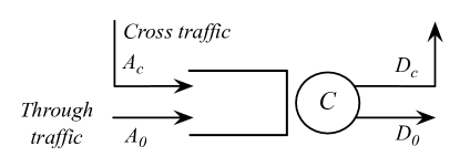
Figure 1: Buffered link with fixed capacity $C$ and cross traffic.

III Networks of $\Delta$-Schedulers

In this section, we obtain a statistical network service curve that describes the service available on an end-to-end path of network links, where each link realizes a packet scheduling algorithm. To characterize link schedulers, we use a general description of scheduling algorithms, referred to as $\Delta$-scheduling, recently developed in [14].

III-A $\Delta$-Schedulers

Consider a buffered link with a fixed capacity of rate $C$ and without buffer size constraints as shown in Fig. 1. We are interested in describing the performance of a (through) flow with arrival function $A_{0}$ at this link. The flow experiences cross traffic from a flow with arrival function $A_{c}$. We do not assume independence of through and cross traffic. On the contrary, the traffic can be correlated in an adversarial fashion. A scheduling algorithm at the link determines the order of transmission of backlogged traffic.

We consider the class of work-conserving scheduling algorithms whose operation can be entirely described by a set of constants $\Delta_{ij}$ where $i$ and $j$ indicate flow indices. For two backlogged packets $p_{i}$ and $p_{j}$ from flows $i$ and $j$, the scheduler selects $p_{i}$ over $p_{j}$ for transmission, if $p_{j}$ arrives more than $\Delta_{ij}$ time units after $p_{i}$. Schedulers that can be described in this fashion are referred to as $\Delta$-schedulers. Special cases are FIFO ($\Delta_{ij}=0,\forall i,j$) and Static Priority ($\Delta_{ij}=\infty$, if the priority of flow $i$ is lower than that of flow $j$, and $\Delta_{ij}=-\infty$, if the priority of flow $i$ is higher than that of flow $j$). A $\Delta$-scheduler with non-zero but finite values of $\Delta_{ij}$ can be implemented by an algorithm that tags each packet arrival with a timestamp consisting of the sum of the arrival time and a flow-specific value (e.g., a target delay), and transmits packets in the order of timestamps. Here, the value of $\Delta_{ij}$ is the difference of the tags assigned to through and cross traffic. For example, the Earliest-Deadline-First can be realized by setting $\Delta_{ij}=d^{*}_{i}-d^{*}_{j}$, where $d^{*}_{i}$ and $d^{*}_{j}$ are the a priori delay bounds of flows $i$ and $j$.

For any $\Delta$-scheduler operating at a buffered link with capacity $C$ where the cross traffic is bounded by a statistical sample path envelope given by ${\cal G}_{c}(t;\sigma)$ and $\varepsilon_{c}(\sigma)$, it was shown in [14] that, for any choice of $\theta\geq 0$, the function

$${\cal S}(t;\sigma)=\Bigl{[}Ct-{\cal G}_{c}(t-\theta+\Delta(\theta);\sigma)\Bigr{]}_{+}I_{t>\theta}\ ,$$ (16)

is a statistical service curve with bounding function $\varepsilon_{c}(\sigma)$, and $I_{\rm expr}$ denotes the indicator function, with $I_{\rm expr}=1$ if the expression ‘${\rm expr}$’ is true, and $I_{\rm expr}=0$ otherwise. Also, $\Delta(\theta)=\min\{\theta,\Delta\}$, where $\Delta$ is the constant for the precedence of the through traffic with arrival function $A_{0}$ relative to the cross traffic with arrival function $A_{c}$. (Note: We denote $\Delta=\Delta_{0c}$ since we only work with the constant for arrivals $A_{0}$ relative to $A_{c}$.) For a single node, the service curve characterization from Eq. (16) was shown to yield a tight delay analysis, provided that cross traffic and through traffic are characterized by concave deterministic sample path envelopes [14].

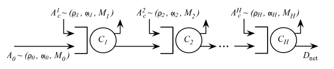
Figure 2: Network path with cross traffic at each link.

III-B A Network Service Curve for $\Delta$-Schedulers

We next apply Theorem 1 to construct a network service curve for $\Delta$-schedulers along a network path as shown in Fig. 2, where the through flow traverses a tandem of $H$ buffered links with $\Delta$-scheduling, and with cross traffic. The arrivals of the cross flow and the $\Delta$-scheduler can be different at each link. We use $\Delta^{h}$ to denote the constant of the $\Delta$-scheduler at the $h$-th node. Arrivals to the cross flow at the $h$-th node, $A^{h}_{c}$, conform to an EBB model, as given by Eq. (4), with rate $\rho_{h}$ and exponentially decaying violation probability $\varepsilon_{h}(\sigma)=M_{h}e^{-\alpha_{h}\sigma}$.

Inserting the statistical sample-path envelope for an EBB cross flow from Eq. (5) into Eq. (16), we obtain for the through flow at node $h$ the service curve and the bounding function

$${\cal S}_{h}(t;\sigma_{h}) =\Bigl{[}C_{h}t-\Bigl{(}(\rho_{h}\!+\!\gamma)(t\!-\!\theta_{h}\!+\!\Delta^{h}(\theta_{h}))+\sigma_{h}\Bigr{)}I_{t>\theta_{h}\!-\!\Delta^{h}}\Bigr{]}_{+}I_{t>\theta_{h}},$$

$$\varepsilon_{h}(\sigma_{h}) =M_{h}e\Bigl{(}1+\frac{\rho_{h}}{\gamma}\Bigr{)}e^{-\alpha_{h}\sigma_{h}}\,.$$

Here, $\gamma>0$ is an arbitrary constant. To simplify the computation of the convolution, we replace this service curve with the lower bound

$${\cal S}_{h}(t;\sigma_{h}) =\Bigl{[}C_{h}t-[(\rho_{h}+\gamma)(t-\theta_{h}+\Delta^{h}(\theta_{h}))+\sigma_{h}]_{+}\Bigr{]}_{+}I_{t>\theta_{h}}.$$ (17)

The replacement comes without loss for $\Delta^{h}\geq 0$, and a reduction by at most $(C_{h}-\rho_{h})[\Delta^{h}]_{-}$ for $\Delta^{h}<0$, where we use $[x]_{-}=\max\{-x,0\}$. The key point is that the right hand side of Eq. (17) is concave and strictly increasing in $t$ as soon as it is positive. We apply Theorem 1 with the free parameters set to $\gamma_{h}=\gamma$ and $\tau_{h}=\frac{\alpha_{h}^{-1}}{\sum_{k<H}\alpha_{k}^{-1}}\tau_{\rm net}$ for $h=1,\dots,H-1$, where $\tau_{\rm net}$ and $\gamma$ are chosen below. By Eq. (9),

$${\cal S}_{\rm net}(t;\sigma) =\left[{\cal S}_{1}*\cdots*{\cal S}_{H}*\delta_{\tau_{\rm net}}(t)-(H-1)\gamma t\right]_{+}$$

$$\geq\left[{\cal S}_{1}*\cdots*{\cal S}_{H}-(H-1)\gamma t\right]_{+}*\delta_{\tau_{\rm net}}(t)-(H\!-\!1)\gamma\tau_{\rm net}\,,$$ (18)

where we use $\sigma$ to mean $\sigma=(\sigma_{1},\ldots,\sigma_{H})$. To evaluate the term inside the square brackets in the second line, we may equivalently convolve the functions $[{\cal S}_{h}(t;\sigma)-(H-1)\gamma t]_{+}$. For each of these factors, we write

$$\left[{\cal S}_{h}(t;\sigma_{h})-(H-1)\gamma t\right]_{+}=\left[(C_{h}-(H\!-\!1)\gamma)t-[(\rho_{h}\!+\!\gamma)(t\!-\!\theta_{h}\!+\!\Delta^{h}(\theta_{h}))+\sigma_{h}]_{+}\right]_{+}I_{t>\theta_{h}}\,.$$ (19)

If we choose $\theta_{h}$ large enough so that

$$\underbrace{(C_{h}-(H\!-\!1)\gamma)\theta_{h}-[(\rho_{h}\!+\!\gamma)\Delta^{h}(\theta_{h})+\sigma_{h}]_{+}}_{=:U_{h}}\geq 0\,,$$ (20)

then we can re-write Eq. (19) as

$$\left[{\cal S}_{h}(t;\sigma_{h})-(H-1)\gamma t\right]_{+}=\widetilde{\cal S}_{h}*\delta_{\theta_{h}}(t)\,,$$

with

$$\widetilde{\cal S}_{h}(t;\sigma_{h}) =\min\left\{(C_{h}-(H\!-\!1)\gamma)(t+\theta_{h}),(C_{h}\!-\!\rho_{h}\!-\!H\gamma)t+U_{h}\right\}I_{t>0}\,.$$ (21)

Since each of the $\widetilde{\cal S}_{h}$ is concave and strictly increasing in $t$, their convolution is given by the pointwise minimum

$$\widetilde{{\cal S}}_{\rm net}(t;\sigma) :=\widetilde{{\cal S}}_{1}*\ldots*\widetilde{{\cal S}}_{H}(t;\sigma)=\min_{h=1,\ldots,H}\Bigl{\{}\widetilde{{\cal S}}_{h}(t;\sigma_{h})\Bigr{\}}\,.$$

Using the associativity and commutativity of the min-plus convolution, we obtain from Eq. (18) the network service curve

$${\cal S}_{\rm net}(t;\sigma)\geq\bigl{(}\widetilde{S}_{\rm net}*\delta_{\tau_{\rm net}+\sum_{h=1}^{H}\theta_{h}}\bigr{)}(t)-(H-1)\gamma\tau_{\rm net}\,.$$ (22)

The bounding function is computed with Theorem 1 as

$$\varepsilon_{\rm net}(\sigma) =M_{H}e\Bigl{(}1+\frac{\rho_{H}}{\gamma}\Bigr{)}e^{-\alpha_{H}\sigma_{H}}+\frac{\sum_{h<H}\alpha_{h}^{-1}}{\gamma\tau_{\rm net}}\sum_{h=1}^{H-1}M_{h}e\Bigl{(}1+\frac{\rho_{h}}{\gamma}\Bigr{)}e^{-\alpha_{h}\sigma_{h}}\,.$$

A probabilistic network service curve for a cascade of $\Delta$-schedulers has been computed in [14] by applying a convolution theorem for service curves from [4]. This required to bring the service curves into the form ${\cal S}_{h}(t;\sigma_{h})=[{\cal S}_{h}(t)-\sigma_{h}]_{+}$, which resulted in a pessimistic service curve of the form

$${\cal S}_{h}(t;\sigma_{h}) =\left[C_{h}t-(\rho_{h}\!+\!\gamma)[t-\theta_{h}+\Delta^{h}(\theta_{h})]_{+}-\sigma_{h}\right]_{+}\!I_{t>\theta_{h}}\!.$$

While the difference in the placement of $\sigma_{h}$ compared to Eq. (17) may appear subtle, the evaluation in Sec. VI will show that the service curve together with the new convolution theorem (Theorem 1) results in substantially improved bounds.

IV Output, backlog, and delay bounds

In this section, we apply the performance bounds (from Sec. II-C) with the network service curve for $\Delta$-schedulers (from Sec. III-B) to a through flow that traverses a network as shown in Fig. 2. We will make choices for the free parameters $\theta_{h}$ appearing in Eq. (16), so that we can obtain explicit bounds on the distribution of the output burstiness from the last node, the end-to-end backlog, and the end-to-end delay. The bounds apply to both deterministic (worst-case) and statistical assumptions.

Consider the same network as described in Sec. III. The through traffic is an EBB flow with arrival function $A_{0}\sim(\rho_{0},\alpha_{0},M_{0})$. We assume that the stability condition

$$\rho_{0}<\min_{h=1,\ldots,H}\{C_{h}-\rho_{h}\}\,$$

holds, and choose $\gamma$ such that

$$0<H\gamma<\min_{h=1,\ldots,H}\{C_{h}-\rho_{h}\}-\rho_{0}\,.$$

To formulate the performance bounds, we need to introduce some more notation. Let

$$\alpha_{\rm net} =\Bigl{(}\sum_{h=0}^{H}\alpha_{h}^{-1}\Bigr{)}^{-1}\!\!,C_{\rm net}\!=\!\min_{h=1,\ldots,H}\{C_{h}\},\,\tau_{\rm net}\!=\!\frac{1}{\alpha_{\rm net}C_{\rm net}}\,,$$

$$M_{\rm net} =M_{0}e\Bigl{(}1+\frac{\rho_{0}}{\gamma}\Bigr{)}+M_{H}e\Bigl{(}1+\frac{\rho_{H}}{\gamma}\Bigr{)}+\frac{C_{\rm net}}{\gamma}\sum_{h=1}^{H-1}M_{h}e\Bigl{(}1+\frac{\rho_{h}}{\gamma}\Bigr{)}\,,$$ (23)

and choose

$$\sigma_{h}=\frac{\alpha_{\rm net}}{\alpha_{h}}\sigma\,,\quad h=0,\dots,H\,.$$

For any given value of $\sigma$, the smallest value of $\theta_{h}$ that makes $\widetilde{\cal S}_{h}(t)>0$ for all $t>0$ (see Eq. (21)) is given by

$$\theta^{*}_{h}=\min\left\{\frac{\sigma_{h}}{C_{h}-\rho_{h}-H\gamma},\frac{[\sigma_{h}+(\rho_{h}+\gamma)\Delta^{h}]_{+}}{C_{h}-(H-1)\gamma}\right\}\,,$$ (24)

and the corresponding value for $U_{h}$ is given by

$$U^{*}_{h}=[\sigma_{h}+(\rho_{h}+\gamma)\Delta^{h}]_{-}\,.$$ (25)

For the network in Fig. 2, let $D_{\rm net}$ denote the output of the through traffic from the last ($H$-th) node. Let $B_{\rm net}(t)=D_{\rm net}(t)-A_{0}(t)$ and $W_{\rm net}(t)$, respectively, denote the total backlog and delay of the through traffic in the network of $H$ nodes.

Theorem 2 (Closed-form Bounds)

With the above notation and definitions, the following bounds hold.

$\bullet$ Output Burstiness:

$${\mathsf{P}}\bigl{(}D_{\rm net}(s,t)-(\rho_{0}+\gamma)(t-s)>b_{\rm net}(\sigma)\bigr{)}\leq M_{\rm net}e^{-\alpha_{\rm net}\sigma}\,,$$

where

$$b_{\rm net}(\sigma) =(\rho_{0}+H\gamma)\tau_{\rm net}+\sigma_{0}+(\rho_{0}+\gamma)\sum_{h=1}^{H}\theta^{*}_{h}\,;$$

$\bullet$ End-to-end backlog:

$${\mathsf{P}}\bigl{(}B_{\rm net}(t)>b_{\rm net}(\sigma)\bigr{)}\leq M_{\rm net}e^{-\alpha_{\rm net}\sigma}\,;$$

$\bullet$ End-to-end delay:

$${\mathsf{P}}\bigl{(}W_{\rm net}(t)>d_{\rm net}(\sigma)\bigr{)}\leq M_{\rm net}e^{-\alpha_{\rm net}\sigma}\,,$$

where

$$d_{\rm net}(\sigma) =\tau_{\rm net}+\max_{h=1,\dots,H}\Bigr{\{}\max\Bigl{\{}\frac{\sigma_{0}+(H-1)\gamma\tau_{\rm net}}{C_{h}-(H-1)\gamma},\frac{\sigma_{0}+(H-1)\gamma\tau_{\rm net}-U^{*}_{h}}{C_{h}-\rho_{h}-H\gamma}\Bigr{\}}\Bigr{\}}+\sum_{h=1}^{H}\theta^{*}_{h}\,.$$

The output bound shows that the departing traffic satisfies the EBB model. In the expressions for $b_{\rm net}(\sigma)$ and $d_{\rm net}(\sigma)$, the second term quantifies the contribution of the through flow’s burstiness to the delay at the bottleneck link, and the last term sums up the contributions of the burstiness of the cross flows. On long paths, i.e., for $H$ large, the last term will dominate the second term.

An important observation is that all bounds increase with $\Delta^{h}$, and that the difference between end-to-end delay and backlog bounds for different schedulers grows linearly with the number of nodes. This clearly indicates that the impact of the scheduling algorithm on end-to-end performance bounds does not diminish on long network paths for these schedulers.

In a discrete-time setting (where $t=0,1,\ldots$), the bounds in the theorem hold with $\tau_{\rm net}=0$, and with Eq. (23) replaced by

$$M_{\rm net} =\frac{M_{0}}{1-e^{-\alpha_{0}\gamma}}+\frac{M_{H}}{1-e^{-\alpha_{H}\gamma}}+\sum_{h=1}^{H-1}\frac{M_{h}}{(1-e^{-\alpha_{h}\gamma})^{2}}\,.$$

Proof:

We insert the network service curve from Theorem 1 into the performance bounds from Sec. II-C. Since $\alpha_{h}\tau_{h}\leq 1/C_{\rm net}$, the bounding function evaluates to $\varepsilon_{0}(\sigma_{0})+\varepsilon_{\rm net}(\sigma)=M_{\rm net}e^{-\alpha_{\rm net}\sigma}\,.$

The backlog bound is given by $b_{\rm net}(\sigma)={\cal G}_{0}\oslash S_{\rm net}(0)$. For $\theta_{h}\geq\theta^{*}_{h}$, we compute this deconvolution as

$$b_{\rm net}(\sigma) ={\cal G}_{0}\oslash\left[\bigl{(}\widetilde{S}_{\rm net}*\delta_{\tau_{\rm net}+\sum_{h=1}^{H}\theta_{h}}\bigr{)}-(H\!-\!1)\gamma\tau_{\rm net}\right]_{+}\!(0)$$

$$\leq{\cal G}_{0}\Bigl{(}\tau_{\rm net}+\sum_{h=1}^{H}\theta_{h}\Bigr{)}+(H-1)\gamma\tau_{\rm net}\,.$$ (26)

In the first line, we have used our representation for the network service curve from Eq. (22). The key step is the second line, where we use that $\widetilde{{\cal S}}_{\rm net}$ is concave and ${\cal G}_{0}$ is convex for $t>0$, and that ${\cal G}_{0}(t)<{\cal S}_{\rm net}(t)$ for $t$ is sufficiently large by the stability condition and our choice of $\gamma$. Plugging in $\theta_{h}=\theta^{*}_{h}$, we obtain the desired backlog bound. The same computation gives the bound on the output burstiness.

We turn to the delay bound. For $\theta_{h}\geq\theta^{*}_{h}$, the delay bound from Theorem 2 is given by

$$d_{\rm net}(\sigma)=\min\{d\geq 0\mid\forall t\geq 0:{\cal S}_{\rm net}(t+d;\sigma)\geq{\cal G}_{0}(t;\sigma_{0})\}\,.$$

By Eq. (22), and using as above the concavity of $\widetilde{{\cal S}}_{\rm net}$ and the stability assumption, we arrive at

$$d_{\rm net}(\sigma) =\tau_{\rm net}+\sum_{h=1}^{H}\theta_{h}+\min\Bigl{\{}X\geq 0\mid\widetilde{{\cal S}}_{\rm net}(X)\geq\sigma_{0}+(H-1)\gamma\tau_{\rm net}\Bigr{\}}\,.$$ (27)

Expressing the function $\widetilde{{\cal S}}_{\rm net}$ in terms of the $\widetilde{{\cal S}}^{h}$, we see that the minimum is assumed for

$$X =\max_{h=1,\dots,H}\Bigl{\{}\max\Bigl{\{}\frac{\sigma_{0}+(H-1)\gamma\tau_{\rm net}}{C_{h}-(H-1)\gamma}-\theta_{h},\frac{\sigma_{0}+(H-1)\gamma\tau_{\rm net}-U_{h}}{C_{h}-\rho_{h}-H\gamma}\Bigr{\}}\Bigr{\}}\,.$$

Inserting $\theta_{h}=\theta^{*}_{h}$ and $U_{h}=U^{*}_{h}$ for $h=1,\dots,H$ completes the proof. ∎

We note that $\theta_{h}=\theta^{*}_{h}$ is the optimal choice for the backlog and output bounds. To see this, observe that a selection in the range $0\leq\theta_{h}<\theta^{*}_{h}$ decreases $\widetilde{\cal S}_{h}$, resulting in a smaller network service curve. On the other hand, from Eq. (26) it is apparent that $b_{\rm net}(\sigma)$ increases for $\theta_{h}>\theta^{*}_{h}$. We will see in the next section that the backlog bound is highly accurate, and in many cases tight.

For the delay bound in Eq. (27), the optimal choice for $\theta_{h}$ is not obvious, since $U_{h}$ can be increased by taking $\theta_{h}>\theta^{*}_{h}$, which may result in a smaller value for $d_{\rm net}(\sigma)$. The choice $\theta_{h}=\theta^{*}_{h}$ is clearly suboptimal when $C_{h}-\rho_{h}$ is small and the path is short, i.e., when the cross traffic consumes most of the bandwidth. In the case of a single node ($H=1$) and deterministic arrival bounds, choosing $\theta_{1}=d_{\rm net}$ recovers known necessary and sufficient conditions for delay bounds e.g., [5]. For long paths ($H>1$ large), it is plausible that the choice $\theta_{h}=\theta^{*}_{h}$, which is optimal for backlog and output, also leads to acceptable delay bounds. We will see in the next section that this is indeed the case.

Stronger delay bounds than those stated in the theorem can be obtained by solving the following optimization problem:

$$\mbox{minimize}\quad d_{\rm net}(\sigma)=\tau_{\rm net}+X+\sum_{h=1}^{H}\theta_{h}\ ,$$ (28)

subject to the constraints that $X\geq 0$ and

$$\forall h:\begin{cases}&(C_{h}-(H\!-\!1)\gamma)(X+\theta_{h})\geq\sigma_{0}+(H-1)\gamma\tau_{\rm net}\,,\\ &(C_{h}-\rho_{h}-H\gamma)X+U_{h}\geq\sigma_{0}+(H-1)\gamma\tau_{\rm net}\,,\\ &\theta_{h}\geq\theta_{h}^{*}\,,\end{cases}$$

where $U_{h}$ and $\theta_{h}^{*}$ are defined in Eqs. (20) and (24). This optimization problem is convex if all $\Delta^{h}$ are non-positive, but convexity does not hold if $\Delta^{h}>0$ for at least one node. Nevertheless, the problem is tractable, because the objective function is linear in the variables $X$ and $\theta_{1},\dots,\theta_{H}$. We will see in the evaluation that this optimization sometimes (i.e., for $H$ small) improves the closed-form delay bound of Theorem 2. For FIFO networks (all $\Delta^{h}=0$) and deterministic traffic ($\gamma=\tau_{\rm net}=0$) the optimization recovers existing deterministic end-to-end delay bound for feedforward networks in [8, 12].

V Tightness of End-to-end Bounds

We now address the tightness of the bounds in Theorem 2. We consider the same network as in the previous section, but assume a deterministic context, where the arrivals of the through traffic and cross traffic at the $h$-th node satisfy the deterministic sample path envelopes $E_{0}(t)=\sigma_{0}+\rho_{0}t$ and $E_{h}(t)=\sigma_{h}+\rho_{h}t$ ($t>0$), respectively. We denote a deterministic sample path envelope for the departing through traffic at the $H$-th node by $E_{\rm net}(t)$. We obtain worst-case bounds by setting $\gamma=\tau_{\rm net}=0$ in the expressions for $\theta^{*}_{h}$ in Eq. (24) and $U^{*}_{h}$ in Eq. (25), yielding

$$\theta^{*}_{h}=\min\left\{\frac{\sigma_{h}}{C_{h}-\rho_{h}},\frac{[\sigma_{h}+\rho_{h}\Delta^{h}]_{+}}{C_{h}}\right\}\,,$$

and

$$U^{*}_{h}=[\sigma_{h}+\rho_{h}\Delta^{h}]_{-}\,.$$

Also, setting $\gamma=\tau_{\rm net}=0$ in Theorem 2, we obtain the following bounds, denoted by $E^{*}_{\rm net},b^{*}_{\rm net}$, and $d^{*}_{\rm net}$.

• Output Burstiness:

  $$E^{*}_{\rm net}(t)=\sigma_{0}+\rho_{0}\sum_{h=1}^{H}\theta^{*}_{h}+\rho_{0}t\,;$$

• End-to-end backlog:

  $$b^{*}_{\rm net}=\sigma_{0}+\rho_{0}\sum_{h=1}^{H}\theta^{*}_{h}\,;$$ (29)

• End-to-end delay:

  $$d^{*}_{\rm net}=\max_{h=1,\dots,H}\Bigl{\{}\max\Bigl{\{}\frac{\sigma_{0}}{C_{h}},\frac{\sigma_{0}-U^{*}_{h}}{C_{h}-\rho_{h}}\Bigr{\}}\Bigr{\}}+\sum_{h=1}^{H}\theta^{*}_{h}\,.$$ (30)

For the special cases of priority scheduling where through traffic has lower priority ($\Delta^{h}=+\infty$) or higher priority ($\Delta^{h}=-\infty$), we obtain

$$W_{\rm net}(t)\leq\begin{cases}\displaystyle{\frac{\sigma_{0}}{\min\{C_{h}-\rho_{h}\}}+\sum_{h=1}^{H}\frac{\sigma_{h}}{C_{h}\!-\!\rho_{h}}\,,}&\Delta^{h}=+\infty\,,\\ \displaystyle{\frac{\sigma_{0}}{\min\{C_{h}\}}\,,}&\Delta^{h}=-\infty\,.\end{cases}$$

These bounds are known to be tight, which can be verified with elementary methods of the deterministic network calculus [11].

In the remainder of this section, we evaluate the tightness of the bounds for $\Delta$-schedulers with finite values of $\Delta$. For this, we consider specific adversarial sample path scenarios for through and cross traffic, and compute the maximal observed end-to-end delay and backlog. For any specific arrival scenario, let $B_{\rm max}=\max_{t}\{B_{\rm net}(t)\}$ and $W_{\rm max}=\max_{t}\{W_{\rm net}(t)\}$ denote the maximal end-to-end backlog and delay, respectively, of the through traffic. Clearly, any $B_{\rm max}$ and $W_{\rm max}$, respectively, are lower bounds for the worst-case end-to-end backlog and delay.

Theorem 3 (Tightness of Bounds)

For $-\infty<\Delta^{h}<\infty$, there exists a scenario of through and cross traffic that satisfies the assumptions stated above, such that

$$B_{\rm max} \geq\sigma_{0}+\rho_{0}\sum_{h=1}^{H}L_{h}\,,$$ (31)

$$W_{\rm max} \geq\frac{\sigma_{0}}{\min_{h}\{C_{h}\}}+\sum_{h=1}^{H}L_{h}\,,$$ (32)

with

$$\!\!\!L_{h}=\min\left\{\frac{\sigma_{h}}{C_{h}-\rho_{h}},\frac{[\sigma_{h}+\rho_{h}[\Delta^{h}]_{+}-C_{h}[\Delta^{h}]_{-}]_{+}}{C_{h}}\right\}.$$ (33)

The theorem implies that the backlog bound in Eq. (29) is sharp when $\Delta^{h}\geq 0$ for $h=1,\dots,H$, and, in particular, for FIFO. For $\Delta^{h}<0$, observe that Eq. (33) implies that

$$0\leq\theta^{*}_{h}-L_{h}\leq(1-\frac{\rho_{h}}{C_{h}})[\Delta^{h}]_{-}\ .$$

Here, the deviation $\theta^{*}_{h}-L_{h}$ is due to the relaxation of the service curve in Eq. (17). The delay bound, although not sharp, describes actual delays in adversarial scenarios rather well, particularly on long paths. We conjecture that an optimal choice of the $\theta_{h}$ would result in a delay bound that is as good as the backlog bound.

Proof:

For the arrivals at the first node, we set

$$A_{0}(t)=E_{0}(t)\,.$$

We time the cross traffic to have a maximal burst just before time $t=0$, if $\Delta^{1}\geq 0$, and just before $t=\Delta^{1}$, if $\Delta^{1}<0$, resulting in

$$A^{1}_{c}(t)=E_{1}(t+\nu-[\Delta^{1}]_{-})\,,$$

where $\nu>0$ is an infinitesimally small number.

A careful analysis of the backlog from the cross flow at time $t=[\Delta^{1}]_{+}$, yields that the first bit of the through flow experiences a latency of $L_{1}$. We can construct similar scenarios for cross traffic arrivals at subsequent nodes. For the $h$-th node, we time the arrival of a cross traffic burst relative to the arrival of the first bit of through traffic, by setting

$$A_{c}^{h}(t)=E_{h}\bigl{(}t+\nu-\sum_{k=1}^{h-1}L_{k}-[\Delta^{h}]_{-}\bigr{)}\,.$$

Then, the initial latency of the through flow is increased at the $h$-th node by $L_{h}$. It follows that the first bit of the through flow departs from the last node at time $\sum_{h=1}^{H}L_{h}$, and so

$$B_{\rm max}\geq E_{0}\bigl{(}\sum_{h=1}^{H}L_{h}\bigr{)}\ ,$$

proving Eq. (31). Now, consider the delay of the initial burst of the through flow. From the backlog analysis, we know that the first bit of the burst experiences a delay of $\sum_{h=1}^{H}L_{h}$. Since the rest of the burst cannot be transmitted faster than at the rate of the slowest link, we obtain Eq. (32). ∎

VI Evaluation

We present a numerical evaluation of the end-to-end bounds derived in this paper for deterministic and statistical arrival scenarios. We consider a network as in Fig. 2, where we assume for simplicity that all nodes have the same capacity of $C=100$ Mbps and use the same $\Delta$-scheduler. We use a discrete-time setting with a step size of 1 ms. The traffic arrivals of a flow follow an alternation of On and Off phases, where, in the On phase, a flow transmits at rate $P=1.5$ Mbps, and the long term average arrival rate is $\rho=0.15$ Mbps. The total traffic load at each node is set to 600 flows with $N_{0}=10$ through flows and $N_{c}=590$ cross flows, resulting in a link utilization of $90$%.

For deterministic arrival scenarios, we characterize flows by a deterministic sample path envelope $E(t)=\rho t+\sigma$. We choose the value of $\sigma$ such that the aggregate burstiness of all cross flows is 300 Kb, and likewise for the through flows. (Selecting equal burst sizes for aggregate through and cross traffic provides a good separation of our upper and lower bounds for worst-case end-to-end delays.) Note that the deterministic scenario does not account for statistical multiplexing, i.e., the burst size of $N$ flows is $N$ times the burst of one flow.

For statistical traffic, we assume that the arrivals of each flow are given by a discrete-time Markov-Modulated On-Off process, with an On state ($=1$) and an Off state ($=0$). The probabilities to change states are given by $p_{1\to 0}=0.9$ and $p_{0\to 1}=0.1$. The EBB characterization for the aggregate through and cross traffic can be obtained using the effective bandwidth $eb(\alpha)$ from (e.g., [3], page 292), resulting in EBB parameters for the aggregate through traffic of $\rho_{0}=N_{0}eb(\alpha_{0})$, $M_{0}=1$, and $\alpha_{0}$ selected to achieve high statistical multiplexing gain. The parameters for the cross traffic are chosen accordingly.

We assume that the through flows are independent of each other, and that the cross flows are independent; however, through and cross traffic is not independent. Thus, we observe statistical multiplexing for the group of through flows and the group of cross flows, but not across the groups.

For the discussion of the examples, recall that $\Delta=0$ corresponds to FIFO, $\Delta=\infty$ to priority scheduling with low priority for through traffic, and $\Delta=-\infty$ to priority scheduling with high priority for through traffic.

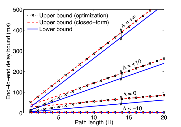
Figure 3: Deterministic end-to-end delay bounds of through traffic.

VI-A Tightness of Delay Bounds

We evaluate the tightness of our delay bounds for the deterministic arrival scenario described above. We compute the end-to-end delay bounds of the through traffic for different $\Delta$-schedulers as a function of the number of nodes $H$. We present the closed-form delay bound $d^{*}_{\rm net}$ according to Eq. (30), the bound computed with the optimization according to Eq. (28) (with $\tau_{\rm net}=\gamma=0$, since we are in a deterministic scenario), and the lower bound for the worst-case delay from Eq. (32).

The results are shown in Fig. 3. The closed-form delay bounds track the bounds from the optimization very closely, and are virtually identical for long paths. Both upper bounds are highly accurate compared to the lower bound on the worst-case delay. Note that the differences between the delay bounds for different scheduling algorithms increase proportionally to the number of traversed nodes. Thus, in contrast to the scenario discussed in the introduction of the paper, we observe that the impact of scheduling is just as strong on long paths as on a single node.

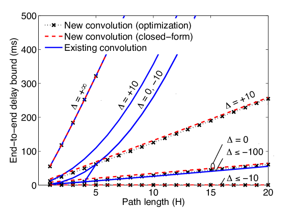
Figure 4: Statistical end-to-end delay bounds ($\varepsilon=10^{-9}$).

VI-B Improvement due to Theorem 1

For the remaining examples, we use the statistical traffic scenario. We first evaluate the benefit our convolution result, by comparing statistical delay bounds computed with the previously best convolution result from [4], to the delay bounds obtained with the new convolution result in Theorem 1. The delay bound computation for $\Delta$-schedulers with the convolution result from [4] uses an optimization, which is described in [14]. For delay bounds computed with Theorem 1, we evaluate the closed-form expression from Theorem 2, as well as the optimization in Eq. (28). We use a fixed violation probability of $\varepsilon=10^{-9}$.

In Fig. 4, we show the end-to-end delay bounds of the through traffic for different $\Delta$-schedulers for increasing path length. In all cases, the closed-form delay bounds are very close to the bounds obtained by the optimization. For $\Delta=\infty$, i.e., a priority scheduler where through traffic has lowest priority, the delay bounds obtained with the new convolution theorem give the same results as [4]. Otherwise, the new convolution theorem results in dramatically improved delay bounds, especially for long paths. Our results clearly motivate the need for our new statistical network service curve expression for schedulers with $\Delta<\infty$. In fact, the delay bounds obtained with the ‘old’ convolution method for service curves show a similar growth rate for large $H$, thus, systematically underestimating the difference between schedulers.

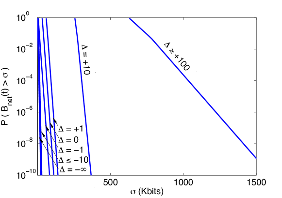
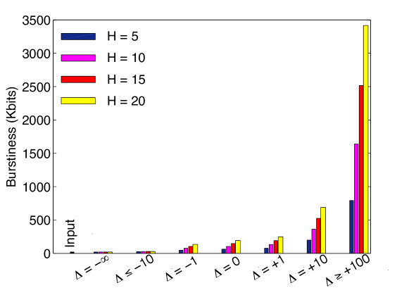
Figure 5: Tail bound of backlog distribution ($H=10$).

Figure 6: Burst size of output traffic ($\varepsilon=10^{-9}$).

VI-C Tail Bound of Backlog Distribution

Fig. 6 shows the tail distribution for the backlog of the through traffic for a path of $H=10$ nodes. The graph shows that the backlog distribution divides the $\Delta$-schedulers into two groups: one for large values of $\Delta$, and one for small and negative values of $\Delta$. In the first group, through traffic is treated effectively as low-priority traffic. The second group has a backlog distribution similar to FIFO ($\Delta=0$), indicating that this desirable property of FIFO scheduling extends to some non-FIFO algorithms.

VI-D Burstiness Increase of Output Traffic

Studying the burstiness of the output traffic further corroborates the findings of the previous example. Here, we compute bounds for the output of the through traffic for different choices of $\Delta$ and $H$, by applying the closed-form bound for $D_{\rm net}$ from Theorem 2.

In Fig. 6 we show the burst size of the output bound for a violation probability $\varepsilon=10^{-9}$ in a bar chart. (The rate values are omitted since the long-term traffic rate does not change at the output of a link.) For comparison, the leftmost bar shows the burst of the through traffic arrivals at the first node. For large values of $\Delta$, we see that the burstiness increases sharply. For values of $\Delta$ close to zero or negative, we observe only a modest increase of the burstiness at the output, even when the number of nodes is large. As a result, the arrival process at downstream nodes is not markedly different from that at the first node. Since modest increases of output burstiness are an important condition for a network decomposition analysis, e.g., see [7, 18], our work suggests that conditions for decomposition may not be limited to FIFO networks.

VII Conclusions

The analytical methods and closed-form expression developed in this paper vastly enhance available methods for end-to-end performance analysis in networks with deterministic and statistical traffic. With our analysis, it is now possible to make conclusive statements about the role of link scheduling in large networks. Contrary to conventional wisdom, we showed that the impact of link scheduling generally does not diminish on long network paths. We also shed light on a group of scheduling algorithms that provide service differentiation without the penalties of strict priority scheduling in terms of buffer requirements and deterioration of the burstiness of traffic.

References

- [1] T. Bonald, A. Proutiere, and J. W. Roberts. Statistical guarantees for streaming flows using expedited forwarding. In Proc. IEEE Infocom, pages 1104–1112, April 2001.
- [2] C.-S. Chang. Stability, queue length, and delay of deterministic and stochastic queueing networks. IEEE Trans. on Automatic Control, 39(5):913–931, May 1994.
- [3] C.-S. Chang. Performance Guarantees in Communication Networks. Springer Verlag, 2000.
- [4] F. Ciucu, A. Burchard, and J. Liebeherr. Scaling properties of statistical end-to-end bounds in the network calculus. IEEE Trans. on Information Theory, 52(6):2300–2312, June 2006.
- [5] R. Cruz. A calculus for network delay, parts I and II. IEEE Trans. on Information Theory, 37(1):114–141, January 1991.
- [6] R. L. Cruz. Quality of service guarantees in virtual circuit switched networks. IEEE J. on Selected Areas in Communications, 13(6):1048–1056, August 1995.
- [7] D. Y. Eun and N. B. Shroff. Network decomposition: Theory and practice. IEEE/ACM Trans. on Networking, 13(3):526–539, June 2005.
- [8] M. Fidler. Extending the network calculus pay bursts only once principle to aggregate scheduling. In Proc. QoS-IP’03, pages 19–34, Feb. 2003.
- [9] Y. Ghiassi-Farrokhfal and J. Liebeherr. Output characterization of constant bit rate traffic in FIFO networks. IEEE Communications Letters, 13(8):618–620, Aug. 2009.
- [10] Y. Jiang and Y. Liu. Stochastic Network Calculus. Springer, 2008.
- [11] J. Y. Le Boudec and P. Thiran. Network Calculus. Springer, 2001.
- [12] L. Lenzini, E. Mingozzi, and G. Stea. Delay bounds for FIFO aggregates: A case study. Computer Comm., 28(3):287–299, Feb. 2005.
- [13] J. Liebeherr, A. Burchard, and F. Ciucu. Non-asymptotic delay bounds for networks with heavy-tailed traffic. In Proc. IEEE Infocom, pages 1325–1333, March 2010.
- [14] J. Liebeherr, Y. Ghiassi-Farrokhfal, and A. Burchard. Does link scheduling matter on long paths? In Proc. IEEE ICDCS, pages 199–208, June 2010.
- [15] B. Melander, M. Bjorkman, and P. Gunningberg. First-come-first-served packet dispersion and implications for TCP. In Proc. IEEE GLOBECOM, pages 2170–2174, Nov. 2002.
- [16] D. Starobinski and M. Sidi. Stochastically bounded burstiness for communication networks. IEEE Trans. on Information Theory, 46(1):206–212, Jan. 2000.
- [17] O. Yaron and M. Sidi. Performance and stability of communication networks via robust exponential bounds. IEEE/ACM Trans. on Networking, 1(3):372–385, June 1993.
- [18] Y. Ying, R. Mazumdar, C. Rosenberg, and F. Guillemin. The burstiness behavior of regulated flows in networks. In Proc. 4th IFIP Networking 2005, pages 918–929, May 2005.
- [19] H. Zhang. Service disciplines for guaranteed performance service in packet-switching networks. Proceedings of the IEEE, 83(10):1374–1396, Oct. 1995.