Uniform convergence and a posteriori error estimation for assumed stress hybrid finite element methods

Abstract:    Assumed stress hybrid methods are known to improve the performance of standard displacement-based finite elements and are widely used in computational mechanics. The methods are based on the Hellinger-Reissner variational principle for the displacement and stress variables. This work analyzes two existing 4-node hybrid stress quadrilateral elements due to Pian and Sumihara [Int. J. Numer. Meth. Engng, 1984] and due to Xie and Zhou [Int. J. Numer. Meth. Engng, 2004], which behave robustly in numerical benchmark tests. For the finite elements, the isoparametric bilinear interpolation is used for the displacement approximation, while different piecewise-independent 5-parameter modes are employed for the stress approximation. We show that the two schemes are free from Poisson-locking, in the sense that the error bound in the a priori estimate is independent of the relevant Lam$\acute{\mbox{e}}$ constant $\lambda$. We also establish the equivalence of the methods to two assumed enhanced strain schemes. Finally, we derive reliable and efficient residual-based a posteriori error estimators for the stress in $L^{2}$-norm and the displacement in $H^{1}$-norm, and verify the theoretical results by some numerical experiments.

Key words:    Finite element,   Assumed stress hybrid method,    Hellinger-Reissner principle,    Poisson-locking,    A posteriori estimator

1.  Introduction

Let $\Omega\subset\mathbb{R}^{2}$ be a bounded open set with boundary $\Gamma=\Gamma_{D}\bigcup\Gamma_{N}$, where meas($\Gamma_{D}$)$>$0. The plane linear elasticity model is given by

$$\left\{\begin{array}[]{ll}-\mathbf{div}\boldsymbol{\sigma}=\mathbf{f}&\mbox{in}\quad\Omega,\\ \boldsymbol{\sigma}=\mathbb{C}\varepsilon(\mathbf{u})&\mbox{in}\quad\Omega,\\ \mathbf{u}|_{\Gamma_{D}}=0,\boldsymbol{\sigma}\mathbf{n}|_{\Gamma_{N}}=\mathbf{g},\\ \end{array}\right.$$ (1.1)

where $\boldsymbol{\sigma}\in\mathbb{R}^{2\times 2}_{sym}$ denotes the symmetric stress tensor field, $\mathbf{u}\in\mathbb{R}^{2}$ the displacement field, $\varepsilon(\mathbf{u})=(\nabla\mathbf{u}+\nabla^{T}\mathbf{u})/2$ the strain, $\mathbf{f}\in\mathbb{R}^{2}$ the body loading density, $\mathbf{g}\in\mathbb{R}^{2}$ the surface traction, $\mathbf{n}$ the unit outward vector normal to $\Gamma$, and $\mathbb{C}$ the elasticity modulus tensor with

$$\mathbb{C}\varepsilon(\mathbf{u})=2\mu\varepsilon(\mathbf{u})+\lambda\mbox{div}\mathbf{u}\ \mathbf{I},$$

$\mathbf{I}$ the $2\times 2$ identity tensor, and $\mu,\lambda$ the Lam$\acute{\mbox{e}}$ parameters given by $\mu=\frac{E}{2(1+\nu)}$, $\lambda=\frac{E\nu}{(1+\nu)(1-2\nu)}$ for plane strain problems and by $\mu=\frac{E}{2(1+\nu)}$, $\lambda=\frac{E\nu}{(1+\nu)(1-\nu)}$ for plane stress problems, with $0<\nu<0.5$ the Poisson ratio and $E$ the Young’s modulus.

It is well-known that the standard 4-node displacement quadrilateral element (i.e. isoparametric bilinear element) yields poor results at coarse meshes for problems with bending and suffers from ”Poisson locking” for plane strain problems, at the nearly incompressible limit ($\lambda\rightarrow\infty$ as $\nu\rightarrow 0.5$). We refer to [1] for the mathematical characteristic of locking. To improve the performance of the isoparametric bilinear displacement element while preserving its convenience, various methods have been suggested in literature.

The method of incompatible displacement modes is based on enriching the standard displacement modes with internal incompatible displacements. A representative incompatible displacement is the so-called Wilson element proposed by Wilson, Taylor, Doherty, and Ghaboussi [29]. It achieves a greater degree of accuracy than the isoparametric bilinear element when using coarse meshes. This element was subsequently modified by Taylor, Wilson and Beresford [27], and the modified Wilson element behaves uniformly in the nearly incompressibility. In [14], Lesaint analyzed convergence on uniform square meshes for Wilson element. He and Zl$\acute{\mbox{a}}$mal then established convergence for the modified Wilson element on arbitrary quadrilateral meshes [15]. In [26], Shi established a convergence condition for the quadrilateral Wilson element. In [34], Zhang derived uniform convergence for the modified Wilson element on arbitrary quadrilateral meshes.

The assumed-stress hybrid approach is a kind of mixed method based on the Hellinger-Reissner variational principle which includes displacements and stresses. The pioneering work in this direction is by Pian [16], where the assumed stress field assumed to satisfy the homogenous equilibrium equations pointwise. In [17] Pian and Chen proposed a new type of the hybrid-method by imposing the stress equilibrium equations in a variational sense and by adopting the natural co-ordinate for stress approximation. In [18] Pian and Sumihara derived the famous assumed stress hybrid element (abbreviated as the PS finite element) through a rational choice of stress terms. Despite of the use of isoparametric bilinear displacement approximation, the PS finite element yields uniformly accurate results for all the numerical benchmark tests. Pian and Tong [20] discussed the similarity and basic difference between the incompatible displacement model and the hybrid stress model. In the direction of determining the optimal stress parameters, there have been many other research efforts [19, 30, 31, 32, 35]. In [30, 32], Xie and Zhou derived robust 4-node hybrid stress quadrilateral elements by optimizing stress modes with a so-called energy-compatibility condition, i.e. the assumed stress terms are orthogonal to the enhanced strains caused by Wilson bubble displacements. In [36] a convergence analysis was established for the PS element, but the upper bound in the error estimate is not uniform with respect to $\lambda$. So far there is no uniform error analysis with respect to the nearly incompressibility for the assumed stress hybrid methods on arbitrary quadrilateral meshes.

Closely related to the assumed stress method is the enhanced assumed strain method (EAS) pioneered by Simo and Rifai [25]. Its variational basis is the Hu-Washizu principle which includes displacements, stresses, and enhanced strains. It was shown in [25] that the classical method of incompatible displacement modes is a special case of the EAS-method. Yeo and Lee [33] proved that the EAS concept in some model situation is equivalent to a Hellinger-Reissner formulation. In [24], Reddy and Simo established an a priori error estimate for the EAS method on parallelogram meshes. Braess [3] re-examined the sufficient conditions for convergence, in particular relating the stability condition to a strengthened Cauchy inequality, and elucidating the influence of the Lam$\acute{e}$ constant $\lambda$. In [4], Braess, Carstensen and Reddy established uniform convergence and a posteriori estimates for the EAS method on parallelogram meshes.

The main goal of this work is to establish uniform convergence and a posteriori error estimates for two 4-node assumed stress hybrid quadrilateral elements: the PS finite element by Pian and Sumihara [18] and the ECQ4 finite element by Xie and Zhou [30]. Equivalence is established between the hybrid finite element schemes and two EAS proposed schemes. We also carry out an a posteriori error analysis for the hybrid methods.

The paper is organized as follows. In Section 2 we discuss the uniform stability of the weak formulations. Section 3 is devoted to finite element formulations of the hybrid elements PS and ECQ4 and their numerical performance investigation. We establish the uniformly stability conditions and derive uniform a priori error estimates in Section 4. Equivalence between the hybrid schemes and two EAS schemes is discussed in Section 5. We devote Section 6 to an analysis of a posteriori error estimates for the hybrid methods and verification of the theoretical results by numerical tests.

2.   Uniform stability of the weak formulations

First we introduce some notations. Let $L^{2}(T;X)$ be the space of square integrable functions defined on $T$ with values in the finite-dimensional vector space X and with norm being denoted by $||\cdot||_{0,T}$. We denote by $H^{k}(T;X)$ the usual Sobolev space consisting of functions defined on $T$, taking values in $X$, and with all derivatives of order up to $k$ square-integrable. The norm on $H^{k}(T;X)$ is denoted by $||\cdot||_{k,T}:=(\sum_{0\leq j\leq k}|v|_{j,T}^{2})^{1/2},$ with $|\cdot|_{k,T}$ the semi-norm derived from the partial derivatives of order equal to $k$. When there is no conflict, we may abbreviate them to $||\cdot||_{k}$ and $|\cdot|_{k}$. Let $L^{2}_{0}(\Omega)$ be the space of square integrable functions with zero mean values. We denote by $P_{k}(T)$ the set of polynomials of degree less than or equal to $k$, by $Q_{k}$ the set of polynomials of degree less than or equal to $k$ in each variable.

For convenience, we use the notation $a\lesssim b$ to represent that there exists a generic positive constant $C$, independent of the mesh parameter $h$ and the Lam$\acute{e}$ constant $\lambda$, such that $a\leq Cb$. Finally, $a\approx b$ abbreviates $a\lesssim b\lesssim a$.

We define two spaces as follows:

$$V:=H_{D}^{1}(\Omega)^{2}=\{\mathbf{u}\in H^{1}(\Omega)^{2}:\mathbf{u}|_{\Gamma_{D}}=0\},$$

$$\Sigma:=\left\{\begin{array}[]{ll}\mathbf{L}^{2}(\Omega;\mathbb{R}_{sym}^{2\times 2}),&if\,\,meas(\Gamma_{N})>0,\\ \{\boldsymbol{\tau}\in\mathbf{L}^{2}(\Omega;\mathbb{R}_{sym}^{2\times 2}):\int_{\Omega}tr\boldsymbol{\tau}d\mathbf{x}=0\},&if\,\,\Gamma_{N}=\emptyset,\end{array}\right.$$

where $\mathbf{L}^{2}(\Omega;\mathbb{R}_{sym}^{2\times 2})$ denotes the space of square-integrable symmetric tensors with the norm $||\cdot||_{0}$ defined by $||\boldsymbol{\tau}||_{0}^{2}:=\int_{\Omega}\boldsymbol{\tau}:\boldsymbol{\tau}d{\bf x}$, and $tr\boldsymbol{\tau}:=\boldsymbol{\tau}_{11}+\boldsymbol{\tau}_{22}$ represents the trace of the tensor $\boldsymbol{\tau}$. Notice that on the space $V$, the semi-norm $|\cdot|_{1}$ is equivalent to the norm $||\cdot||_{1}$.

The Hellinger-Reissner variational principle for the model (1.1) reads as: Find $(\boldsymbol{\sigma},\mathbf{u})\in\Sigma\times V$ with

$$a(\boldsymbol{\sigma},\boldsymbol{\tau})-\int_{\Omega}\boldsymbol{\tau}:\varepsilon(\mathbf{u})d\mathbf{x}=0\hskip 14.22636pt\,\mbox{for all }\boldsymbol{\tau}\in\Sigma,$$ (2.1)

$$\int_{\Omega}\boldsymbol{\sigma}:\varepsilon(\mathbf{v})d\mathbf{x}=F(\mathbf{v})\,\hskip 36.98866pt\mbox{for all }\mathbf{v}\in V,$$ (2.2)

where

$$a(\boldsymbol{\sigma},\boldsymbol{\tau}): = \int_{\Omega}\boldsymbol{\sigma}:\mathbb{C}^{-1}\boldsymbol{\tau}d\mathbf{x}=\frac{1}{2\mu}\int_{\Omega}\left(\boldsymbol{\sigma}:\boldsymbol{\tau}-\frac{\lambda}{2(\mu+\lambda)}tr\boldsymbol{\sigma}tr\boldsymbol{\tau}\right)d\mathbf{x}$$

$$= \int_{\Omega}\left(\frac{1}{2\mu}\boldsymbol{\sigma}^{D}:\boldsymbol{\tau}^{D}+\frac{1}{4(\mu+\lambda)}tr\boldsymbol{\sigma}tr\boldsymbol{\tau}\right)d\mathbf{x},$$

$$F(\mathbf{v}): = \int_{\Omega}\mathbf{f}\cdot\mathbf{v}d\mathbf{x}+\int_{\Gamma_{N}}\mathbf{g}\cdot\mathbf{v}ds.$$

Here and throughout the paper, $\boldsymbol{\sigma}:\boldsymbol{\tau}=\sum_{i,j=1}^{2}\boldsymbol{\sigma}_{ij}\boldsymbol{\tau}_{ij},$ and $\boldsymbol{\tau}^{D}:=\boldsymbol{\tau}-\frac{1}{2}tr\boldsymbol{\tau}\mathbf{I}$.

The following continuity conditions are immediate:

$$a(\boldsymbol{\sigma},\boldsymbol{\tau})\lesssim||\boldsymbol{\sigma}||_{0}||\boldsymbol{\tau}||_{0},\ \boldsymbol{\sigma},\ \boldsymbol{\tau}\in\Sigma,$$ (2.3)

$$\int_{\Omega}\boldsymbol{\tau}:\varepsilon(\mathbf{v})d\mathbf{x}\lesssim||\boldsymbol{\tau}||_{0}|\mathbf{v}|_{1},\ \boldsymbol{\tau}\in\Sigma,\ \mathbf{v}\in V,$$ (2.4)

$$F(\mathbf{v})\lesssim(||\mathbf{f}||_{-1}+||\mathbf{g}||_{-\frac{1}{2},\Gamma_{N}})|\mathbf{v}|_{1},\ \mathbf{v}\in V.$$ (2.5)

According to the theory of mixed finite element methods [6, 7], we need the following two stability conditions for the well-posedness of the weak problem (2.1)-(2.2).
($\mathrm{A1}$)  Kernel-coercivity: For any $\boldsymbol{\tau}\in Z:=\{\boldsymbol{\tau}\in\Sigma:\int_{\Omega}\boldsymbol{\tau}:\varepsilon(\mathbf{v})d\mathbf{x}=0\ \ \mbox{for all }\mathbf{v}\in V\}$ it holds

$$\|\boldsymbol{\tau}\|_{0}^{2}\lesssim a(\boldsymbol{\tau},\boldsymbol{\tau});$$

($\mathrm{A2}$)  Inf-sup condition: For any $\mathbf{v}\in V$ it holds

$$|\mathbf{v}|_{1}\lesssim\sup_{0\neq\boldsymbol{\tau}\in\Sigma}\frac{\int_{\Omega}\boldsymbol{\tau}:\varepsilon(\mathbf{v})d\mathbf{x}}{\|\boldsymbol{\tau}\|_{0}}.$$

The proof of (A1)-(A2) utilizes a lemma of Bramble, Lazarov and Pasciak.

Lemma 2.1.

([5])  For $q\in L:=\left\{\begin{array}[]{ll}L^{2}(\Omega)&if\,\,meas(\Gamma_{N})>0,\\ L_{0}^{2}(\Omega)&if\,\,\Gamma_{N}=\emptyset\end{array}\right.$ it holds

$$\|q\|_{0}\lesssim\sup\limits_{\mathbf{v}\in V}\frac{\int_{\Omega}q\,{\bf div}\mathbf{v}d\mathbf{x}}{|\mathbf{v}|_{1}}.$$

The following stability result is given in [4] for the model situation $\Gamma_{N}=\emptyset$.

Theorem 2.1.

The uniform stability conditions (A1) and (A2) hold.

Proof.

Firstly we prove (A1). Since

$$a(\boldsymbol{\tau},\boldsymbol{\tau})=\int_{\Omega}\left(\frac{1}{2\mu}\boldsymbol{\tau}^{D}:\boldsymbol{\tau}^{D}+\frac{1}{4(\mu+\lambda)}tr\boldsymbol{\tau}tr\boldsymbol{\tau}\right)d\mathbf{x},$$

we only need to prove $\|tr\boldsymbol{\tau}\|_{0}\lesssim\|\boldsymbol{\tau}^{D}\|_{0}$ for any $\boldsymbol{\tau}\in Z$.

In fact, for $\boldsymbol{\tau}\in Z$ and any $\mathbf{v}\in V$, it holds

$$0 = \int_{\Omega}\boldsymbol{\tau}:\varepsilon(\mathbf{v})d\mathbf{x}=\int_{\Omega}(\frac{1}{2}tr\boldsymbol{\tau}\mathbf{I}+\boldsymbol{\tau}^{D}):\varepsilon(\mathbf{v})d\mathbf{x}$$

$$= \int_{\Omega}\frac{1}{2}tr\boldsymbol{\tau}\mbox{div}\mathbf{v}d\mathbf{x}+\int_{\Omega}\boldsymbol{\tau}^{D}:\varepsilon(\mathbf{v})d\mathbf{x}.$$

Thus, by Lemma 2.1 we obtain

$$\|tr\boldsymbol{\tau}\|_{0}\lesssim\sup\limits_{\mathbf{v}\in V}\frac{\int_{\Omega}tr\boldsymbol{\tau}\ \mbox{div}\mathbf{v}d\mathbf{x}}{|\mathbf{v}|_{1}}=\sup\limits_{\mathbf{v}\in V}\frac{-2\int_{\Omega}\boldsymbol{\tau}^{D}:\varepsilon(\mathbf{v})d\mathbf{x}}{|\mathbf{v}|_{1}}\leq 2\|\boldsymbol{\tau}^{D}\|_{0}.$$

This implies (A1). For the proof of (A2), let $\mathbf{v}\in V$ and notice $\varepsilon(\mathbf{v})\in\Sigma$. Then

$$|\varepsilon(\mathbf{v})|_{0}\leq\sup_{\boldsymbol{\tau}\in\Sigma\setminus\{0\}}\frac{\int_{\Omega}\boldsymbol{\tau}:\varepsilon(\mathbf{v})d\mathbf{x}}{\|\boldsymbol{\tau}\|_{0}}.$$

Hence (A2) follows from the equivalence between the two norms $|\varepsilon(\mathbf{v})|_{0}$ and $|\mathbf{v}|_{1}$ on $V$. ∎

In view of the continuity conditions, (2.3)-(2.5), and the stability conditions, (A1)-(A2), we immediately get the well-posedness results:

Theorem 2.2.

Assume that $\mathbf{f}\in V^{\prime},\ \mathbf{g}\in H^{-1/2}(\Gamma_{N})$. Then the weak problem (2.1)-(2.2) admits a unique solution $(\boldsymbol{\sigma},\mathbf{u})\in\Sigma\times V$ such that

$$||\boldsymbol{\sigma}||_{0}+|\mathbf{u}|_{1}\lesssim||\mathbf{f}||_{-1}+||\mathbf{g}||_{-\frac{1}{2},\Gamma_{N}}.$$

3.  Finite element formulations for hybrid methods

3.1  Geometric properties of quadrilaterals

In what follows we assume that $\Omega$ is a convex polygonal domain. Let $T_{h}$ be a conventional quadrilateral mesh of ${\Omega}$. We denote by $h_{K}$ the diameter of a quadrilateral $K\in T_{h}$, and denote $h:=\max_{K\in T_{h}}h_{K}$. Let $Z_{i}(x_{i},y_{i})$, $1\leq i\leq 4$ be the four vertices of $K$, and $T_{i}$ denotes the sub-triangle of $K$ with vertices $Z_{i-1}$, $Z_{i}$ and $Z_{i+1}$ (the index on $Z_{i}$ is modulo 4). Define

$$\rho_{K}=\min\limits_{1\leq i\leq 4}\ \mathrm{diameter\ of\ circle\ inscribed\ in}\ T_{i}.$$

Throughout the paper, we assume that the partition $T_{h}$ satisfies the following ”shape-regularity” hypothesis: There exist a constant $\varrho>2$ independent of $h$ such that for all $K\in T_{h},$

$$h_{K}\leq\varrho\rho_{K}.$$ (3.1)

Remark 3.1.

As pointed out in [34], this shape regularity condition is equivalent to the following one which has been widely used in literature (e.g. [11]): there exist two constants $\varrho^{\prime}>2$ and $0<\gamma<1$ independent of $h$ such that for all $K\in T_{h}$,

$$h_{K}\leq\varrho^{\prime}\rho_{K}^{\prime},\ \ |\cos\theta_{K}^{i}|\leq\gamma\ \ \ \mbox{ for }\ \ 1\leq i\leq 4.$$

Here $\rho_{K}^{\prime}$ and $\theta_{K}^{i}$ denote the maximum diameter of all circles contained in $K$ and the angles associated with vertices of $K$.

Let $\hat{K}=[-1,1]\times[-1,1]$ be the reference square with vertices $\hat{Z}_{i}$, $1\leq i\leq 4$. Then exists a unique invertible mapping $F_{K}$ that maps $\hat{K}$ onto $K$ with $F_{K}(\xi,\eta)\in Q_{1}^{2}(\xi,\eta)$ and $F_{K}(\hat{Z}_{i})=Z_{i}$, $1\leq i\leq 4$ (Figure 1). Here $\xi,\eta\in[-1,1]$ are the local isoparametric coordinates.

Figure 1: The mapping $F_{K}$

This isoparametric bilinear mapping $(x,y)=F_{K}(\xi,\eta)$ is given by

$$x=\sum_{i=1}^{4}x_{i}N_{i}(\xi,\eta),\,\,\,y=\sum_{i=1}^{4}y_{i}N_{i}(\xi,\eta),$$ (3.2)

where

$$N_{1}=\frac{1}{4}(1-\xi)(1-\eta),\,N_{2}=\frac{1}{4}(1+\xi)(1-\eta),\,N_{3}=\frac{1}{4}(1+\xi)(1+\eta),\,N_{4}=\frac{1}{4}(1-\xi)(1+\eta).$$

We can rewrite (3.2) as

$$x=a_{0}+a_{1}\xi+a_{2}\eta+a_{12}\xi\eta,\,\,\,y=b_{0}+b_{1}\xi+b_{2}\eta+b_{12}\xi\eta,$$ (3.3)

where

$$\left(\begin{array}[]{cc}a_{0}&b_{0}\\ a_{1}&b_{1}\\ a_{2}&b_{2}\\ a_{12}&b_{12}\end{array}\right)=\frac{1}{4}\left(\begin{array}[]{cccc}1&1&1&1\\ -1&1&1&-1\\ -1&-1&1&1\\ 1&-1&1&-1\\ \end{array}\right)\left(\begin{array}[]{cc}x_{1}&y_{1}\\ x_{2}&y_{2}\\ x_{3}&y_{3}\\ x_{4}&y_{4}\\ \end{array}\right).$$

Remark 3.2.

Due to the choice of node order (Figure 1), we always have $a_{1}>0,b_{2}>0.$

Remark 3.3.

Notice that when $K$ is a parallelogram, we have $a_{12}=b_{12}=0$, and $F_{K}$ is reduced to an affine mapping.

Then the Jacobi matrix of the transformation $F_{K}$ is

$$DF_{K}(\xi,\eta)=\left(\begin{array}[]{cc}\frac{\partial x}{\partial\xi}&\frac{\partial x}{\partial\eta}\\ \frac{\partial y}{\partial\xi}&\frac{\partial y}{\partial\eta}\\ \end{array}\right)=\left(\begin{array}[]{cc}a_{1}+a_{12}\eta&a_{2}+a_{12}\xi\\ b_{1}+b_{12}\eta&b_{2}+b_{12}\xi\\ \end{array}\right),$$

and the Jacobian of $F_{K}$ is

$$J_{K}(\xi,\eta)=det(DF_{K})=J_{0}+J_{1}\xi+J_{2}\eta,$$

where

$$J_{0}=a_{1}b_{2}-a_{2}b_{1},\,J_{1}=a_{1}b_{12}-a_{12}b_{1},\,J_{2}=a_{12}b_{2}-a_{2}b_{12}.$$

Denote by $F_{K}^{-1}$ the inverse of $F_{K}$, then we obtain

$$\left(\begin{array}[]{cc}\frac{\partial\xi}{\partial x}&\frac{\partial\xi}{\partial y}\\ \frac{\partial\eta}{\partial x}&\frac{\partial\eta}{\partial y}\\ \end{array}\right) = DF_{K}^{-1}\circ F_{K}(\xi,\eta)=(DF_{K})^{-1}$$

$$= \frac{1}{J_{K}(\xi,\eta)}\left(\begin{array}[]{cc}b_{2}+b_{12}\xi&-a_{2}-a_{12}\xi\\ -b_{1}-b_{12}\eta&a_{1}+a_{12}\eta\\ \end{array}\right).$$

It holds the following element geometric properties:

Lemma 3.1.

([34])   For any $K\in T_{h}$, under the hypothesis (3.1), we have

$$\frac{\max\limits_{(\xi,\eta)\in\hat{K}}J_{K}(\xi,\eta)}{\min\limits_{(\xi,\eta)\in\hat{K}}J_{K}(\xi,\eta)}<\frac{h_{K}^{2}}{2\rho_{K}^{2}}\leq\frac{\varrho^{2}}{2},$$ (3.6)

$$\frac{1}{4}\rho_{K}^{2}<a_{1}^{2}+b_{1}^{2}<\frac{1}{4}h_{K}^{2},\ \ \frac{1}{4}\rho_{K}^{2}<a_{2}^{2}+b_{2}^{2}<\frac{1}{4}h_{K}^{2},\ \ a_{12}^{2}+b_{12}^{2}<\frac{1}{16}h_{K}^{2}.$$ (3.7)

In view of the choice of node order (cf. Figure 1), the shape-regular hypothesis (3.1) and the relations (3.7), without loss of generality we assume

$$|b_{1}|\leq a_{1},\ \ |a_{2}|\lesssim b_{2}.$$ (3.8)

Together with (3.7), this leads to

$$a_{1}\approx b_{2}\approx h_{K},\ \ \max\{a_{2},b_{1}\}\lesssim O(h_{K}).$$ (3.9)

Notice also that Lemma 3.1 shows

$$J_{K}\approx J_{0}\approx h_{K}^{2}.$$ (3.10)

3.2  Hybrid methods PS and ECQ4

This subsection is devoted to the finite element formulations of the 4-node assumed stress hybrid quadrilateral elements PS [18] and ECQ4 [30].

Let $\Sigma_{h}\subset\Sigma$ and $V_{h}\subset V$ be finite dimensional spaces respectively for stress and displacement approximations, then the corresponding finite element scheme for the problem (2.1)(2.2) reads as: Find $(\boldsymbol{\sigma}_{h},\mathbf{u}_{h})\in\Sigma_{h}\times V_{h}$, such that

$$a(\boldsymbol{\sigma}_{h},\boldsymbol{\tau})-\int_{\Omega}\boldsymbol{\tau}:\varepsilon(\mathbf{u}_{h})d\mathbf{x}=0\ \ \,\mbox{for all }\boldsymbol{\tau}\in\Sigma_{h},$$ (3.11)

$$\int_{\Omega}\boldsymbol{\sigma}_{h}:\varepsilon(\mathbf{v})d\mathbf{x}=F(\mathbf{v})\,\hskip 28.45274pt\ \ \mbox{for all }\mathbf{v}\in V_{h}.$$ (3.12)

For elements PS and ECQ4, the isoparametric bilinear interpolation is used for the displacement approximation, i.e. the displacement space $V_{h}$ is chosen as

$$V_{h}=\{\mathbf{v}\in V:\hat{\mathbf{v}}=\mathbf{v}|_{K}\circ F_{K}\in Q_{1}(\hat{K})^{2}\ \ \mbox{for all }K\in T_{h}\}.$$ (3.13)

In other words, for $\mathbf{v}=(u,v)^{T}\in V_{h}$ with nodal values $\mathbf{v}(Z_{i})=(u_{i},v_{i})^{T}$ on $K$,

$$\hat{\mathbf{v}}=\sum_{i=1}^{4}\left(\begin{array}[]{l}u_{i}\\ v_{i}\end{array}\right)N_{i}(\xi,\eta)=\left(\begin{array}[]{l}U_{0}+U_{1}\xi+U_{2}\eta+U_{12}\xi\eta\\ V_{0}+V_{1}\xi+V_{2}\eta+V_{12}\xi\eta\end{array}\right),$$ (3.14)

where

$$\left(\begin{array}[]{cc}U_{0}&V_{0}\\ U_{1}&V_{1}\\ U_{2}&V_{2}\\ U_{12}&V_{12}\end{array}\right)=\frac{1}{4}\left(\begin{array}[]{cccc}1&1&1&1\\ -1&1&1&-1\\ -1&-1&1&1\\ 1&-1&1&-1\\ \end{array}\right)\left(\begin{array}[]{cc}u_{1}&v_{1}\\ u_{2}&v_{2}\\ u_{3}&v_{3}\\ u_{4}&v_{4}\\ \end{array}\right).$$

We denote the symmetric stress tensor $\boldsymbol{\tau}:=\left(\begin{array}[]{cc}\boldsymbol{\tau}_{11}&\boldsymbol{\tau}_{12}\\ \boldsymbol{\tau}_{12}&\boldsymbol{\tau}_{22}\\ \end{array}\right)$. For convenience we abbreviate it to $\boldsymbol{\tau}=(\boldsymbol{\tau}_{11},\boldsymbol{\tau}_{22},\boldsymbol{\tau}_{12})^{T}.$ In [18], the 5-parameters stress mode on $\hat{K}$ for the PS finite element takes the form

$$\hat{\boldsymbol{\tau}}=\left(\begin{array}[]{c}\hat{\boldsymbol{\tau}}_{11}\\ \hat{\boldsymbol{\tau}}_{22}\\ \hat{\boldsymbol{\tau}}_{12}\\ \end{array}\right)=\left(\begin{array}[]{ccccc}1&0&0&\eta&\frac{a_{2}^{2}}{b_{2}^{2}}\xi\\ 0&1&0&\frac{b_{1}^{2}}{a_{1}^{2}}\eta&\xi\\ 0&0&1&\frac{b_{1}}{a_{1}}\eta&\frac{a_{2}}{b_{2}}\xi\\ \end{array}\right)\beta^{\tau}\ \ \mbox{for }\beta^{\tau}:=(\beta_{1}^{\tau},\cdots,\beta_{5}^{\tau})^{T}\in\mathbb{R}^{5}.$$ (3.15)

Then the corresponding stress space for the PS finite element is

$$\Sigma_{h}^{PS}:=\left\{\boldsymbol{\tau}\in\Sigma:\ \hat{\boldsymbol{\tau}}=\boldsymbol{\tau}|_{K}\circ F_{K}\mbox{ is of form }(\ref{PSstress1})\ \ \mbox{for all }K\in T_{h}\right\}.$$

In [30], the 5-parameters stress mode on $\hat{K}$ for element ECQ4 has the form

$$\hat{\boldsymbol{\tau}}=\left(\begin{array}[]{c}\hat{\boldsymbol{\tau}}_{11}\\ \hat{\boldsymbol{\tau}}_{22}\\ \hat{\boldsymbol{\tau}}_{12}\\ \end{array}\right)=\left(\begin{array}[]{ccccc}1-\frac{b_{12}}{b_{2}}\xi&\frac{a_{12}a_{2}}{b_{2}^{2}}\xi&\frac{a_{12}b_{2}-a_{2}b_{12}}{b_{2}^{2}}\xi&\eta&\frac{a_{2}^{2}}{b_{2}^{2}}\xi\\ \frac{b_{1}b_{12}}{a_{1}^{2}}\eta&1-\frac{a_{12}}{a_{1}}\eta&\frac{a_{1}b_{12}-a_{12}b_{1}}{a_{1}^{2}}\eta&\frac{b_{1}^{2}}{a_{1}^{2}}\eta&\xi\\ \frac{b_{12}}{a_{1}}\eta&\frac{a_{12}}{b_{2}}\xi&1-\frac{b_{12}}{b_{2}}\xi-\frac{a_{12}}{a_{1}}\eta&\frac{b_{1}}{a_{1}}\eta&\frac{a_{2}}{b_{2}}\xi\\ \end{array}\right)\beta^{\tau}\ \ \mbox{for }\beta^{\tau}\in\mathbb{R}^{5}.$$ (3.16)

Then the corresponding stress space for the ECQ4 finite element is

$$\Sigma_{h}^{EC}:=\left\{\boldsymbol{\tau}\in\Sigma:\ \hat{\boldsymbol{\tau}}=\boldsymbol{\tau}|_{K}\circ F_{K}\mbox{ is of form }(\ref{ECQ4stress1})\ \mbox{ for all }K\in T_{h}\right\}.$$

Remark 3.4.

The stress mode of ECQ4 can be viewed as a modified version of PS mode with a perturbation term:

$$\left(\begin{array}[]{ccccc}1-\frac{b_{12}}{b_{2}}\xi&\frac{a_{12}a_{2}}{b_{2}^{2}}\xi&\frac{a_{12}b_{2}-a_{2}b_{12}}{b_{2}^{2}}\xi&\eta&\frac{a_{2}^{2}}{b_{2}^{2}}\xi\\ \frac{b_{1}b_{12}}{a_{1}^{2}}\eta&1-\frac{a_{12}}{a_{1}}\eta&\frac{a_{1}b_{12}-a_{12}b_{1}}{a_{1}^{2}}\eta&\frac{b_{1}^{2}}{a_{1}^{2}}\eta&\xi\\ \frac{b_{12}}{a_{1}}\eta&\frac{a_{12}}{b_{2}}\xi&1-\frac{b_{12}}{b_{2}}\xi-\frac{a_{12}}{a_{1}}\eta&\frac{b_{1}}{a_{1}}\eta&\frac{a_{2}}{b_{2}}\xi\\ \end{array}\right)$$

$$= \left(\begin{array}[]{ccccc}1&0&0&\eta&\frac{a_{2}^{2}}{b_{2}^{2}}\xi\\ 0&1&0&\frac{b_{1}^{2}}{a_{1}^{2}}\eta&\xi\\ 0&0&1&\frac{b_{1}}{a_{1}}\eta&\frac{a_{2}}{b_{2}}\xi\\ \end{array}\right)+\left(\begin{array}[]{ccccc}-\frac{b_{12}}{b_{2}}\xi&\frac{a_{12}a_{2}}{b_{2}^{2}}\xi&\frac{a_{12}b_{2}-a_{2}b_{12}}{b_{2}^{2}}\xi&0&0\\ \frac{b_{1}b_{12}}{a_{1}^{2}}\eta&-\frac{a_{12}}{a_{1}}\eta&\frac{a_{1}b_{12}-a_{12}b_{1}}{a_{1}^{2}}\eta&0&0\\ \frac{b_{12}}{a_{1}}\eta&\frac{a_{12}}{b_{2}}\xi&-\frac{b_{12}}{b_{2}}\xi-\frac{a_{12}}{a_{1}}\eta&0&0\\ \end{array}\right).$$

Remark 3.5.

When $K\in T_{h}$ is a parallelogram, the stress mode of ECQ4 is reduced to that of PS due to $a_{12}=b_{12}=0$. Thus, PS and ECQ4 are equivalent on parallelogram meshes.

Define the bubble function space

$$B_{h}:=\{\mathbf{v}^{b}\in(L^{2}(\Omega))^{2}:\hat{\mathbf{v}}^{b}(\xi,\eta)=\mathbf{v}^{b}|_{K}\circ F_{K}\in span\{\xi^{2}-1,\eta^{2}-1\}^{2}\ \ \mbox{for all }K\in T_{h}\}.$$ (3.19)

Then for any $\mathbf{v}^{b}\in B_{h}$, we have

$$\hat{\mathbf{v}}^{b}=\mathbf{v}^{b}\circ F_{K}=\left(\begin{array}[]{c}\frac{u_{\xi}}{2}(\xi^{2}-1)+\frac{u_{\eta}}{2}(\eta^{2}-1)\\ \frac{v_{\xi}}{2}(\xi^{2}-1)+\frac{v_{\eta}}{2}(\eta^{2}-1)\\ \end{array}\right)$$ (3.20)

with $u_{\xi},u_{\eta},v_{\xi},v_{\eta}\in R$.

Remark 3.6.

It is easy to know (see [26]) that for any $K\in T_{h}$, $|u_{\xi}|+|u_{\eta}|+|v_{\xi}|+|v_{\eta}|\lesssim|\mathbf{v}^{b}|_{1,K}$.

Define the modified partial derivatives $\frac{\tilde{\partial}v}{\partial x}$, $\frac{\tilde{\partial}v}{\partial y}$, the modified divergence $\tilde{\mbox{div}}\mathbf{v}$ and the modified strain $\tilde{\varepsilon}(\mathbf{v})$ respectively as follows [34]: for $K\in T_{h},$

$$(J_{K}\frac{\tilde{\partial}v}{\partial x}|_{K}\circ F_{K})(\xi,\eta)=\frac{\partial y}{\partial\eta}(0,0)\frac{\partial\hat{v}}{\partial\xi}-\frac{\partial y}{\partial\xi}(0,0)\frac{\partial\hat{v}}{\partial\eta}=b_{2}\frac{\partial\hat{v}}{\partial\xi}-b_{1}\frac{\partial\hat{v}}{\partial\eta},$$

$$(J_{K}\frac{\tilde{\partial}v}{\partial y}|_{K}\circ F_{K})(\xi,\eta)=-\frac{\partial x}{\partial\eta}(0,0)\frac{\partial\hat{v}}{\partial\xi}+\frac{\partial x}{\partial\xi}(0,0)\frac{\partial\hat{v}}{\partial\eta}=-a_{2}\frac{\partial\hat{v}}{\partial\xi}+a_{1}\frac{\partial\hat{v}}{\partial\eta},$$

$$\tilde{\mbox{div}}\mathbf{v}|_{K}=\frac{\tilde{\partial}u}{\partial x}+\frac{\tilde{\partial}v}{\partial y},$$

$$\tilde{\varepsilon}(\mathbf{v})|_{K}=\left(\begin{array}[]{cc}\frac{\tilde{\partial}u}{\partial x}&\frac{1}{2}(\frac{\tilde{\partial}u}{\partial y}+\frac{\tilde{\partial}v}{\partial x})\\ \frac{1}{2}(\frac{\tilde{\partial}u}{\partial y}+\frac{\tilde{\partial}v}{\partial x})&\frac{\tilde{\partial}v}{\partial y}\end{array}\right).$$

It is easy to verify that the PS stress mode satisfies the relation (see [23])

$$\int_{K}\boldsymbol{\tau}:\tilde{\varepsilon}(\mathbf{v}^{b})d\mathbf{x}=0\ \ \,\mbox{for all }\mathbf{v}^{b}\in B_{h},$$ (3.21)

or equivalently

$$\int_{K}(\boldsymbol{\tau}-\boldsymbol{\tau}_{0}):\varepsilon(\mathbf{v}^{b})d\mathbf{x}=0\ \ \,\mbox{for all }\mathbf{v}^{b}\in B_{h}$$

for all $\boldsymbol{\tau}\in\Sigma_{h}^{PS}$, with $\boldsymbol{\tau}_{0}$ the constant part of $\boldsymbol{\tau}$, and that the ECQ4 stress mode satisfies the so-called energy-compatibility condition (see [30, 35])

$$\int_{K}\boldsymbol{\tau}:\varepsilon(\mathbf{v}^{b})d\mathbf{x}=0\ \ \,\mbox{for all }\mathbf{v}^{b}\in B_{h}$$ (3.22)

for all $\boldsymbol{\tau}\in\Sigma_{h}^{EC}$. As a result, the stress spaces $\Sigma_{h}^{PS},\Sigma_{h}^{EC}$ can also be rewritten as

$$\Sigma_{h}^{PS} = \{\boldsymbol{\tau}\in\Sigma:\hat{\boldsymbol{\tau}}_{ij}=\boldsymbol{\tau}_{ij}|_{K}\circ F_{K}\in P_{1}(\xi,\eta),\int_{K}\boldsymbol{\tau}:\tilde{\varepsilon}(\mathbf{v}^{b})d\mathbf{x}=0,$$ (3.23)

$$1\leq i\leq j\leq 2\ \ \mbox{for all }\mathbf{v}^{b}\in B_{h},\ K\in T_{h}\},$$

$$\Sigma_{h}^{EC} = \{\boldsymbol{\tau}\in\Sigma:\hat{\boldsymbol{\tau}}_{ij}=\boldsymbol{\tau}_{ij}|_{K}\circ F_{K}\in P_{1}(\xi,\eta),\int_{K}\boldsymbol{\tau}:\varepsilon(\mathbf{v}^{b})d\mathbf{x}=0,$$ (3.24)

$$1\leq i\leq j\leq 2\ \ \mbox{for all }\mathbf{v}^{b}\in B_{h},\ K\in T_{h}\}.$$

With the continuous isoparametric bilinear displacement approximation $V_{h}$ given in (3.13), the corresponding hybrid finite element schemes for PS and ECQ4 are obtained by respectively taking $\Sigma_{h}=\Sigma_{h}^{PS}$ and $\Sigma_{h}=\Sigma_{h}^{EC}$ in the discretized model (3.11)(3.12).

Remark 3.7.

Since the stress approximation of the hybrid elements is piecewise-independent, the stress parameters, $\beta^{\tau}$ in (3.15) or (3.16), can be eliminated at the element level. In this sense, the computational cost of the hybrid methods is almost the same as that of the isoparametric bilinear element.

3.3.  Numerical performance of hybrid elements

Three test problems are used to examine numerical performance of the hybrid elements PS/ECQ4. The former two are benchmark tests widely used in literature, e.g. [18, 19, 30, 31, 32, 35], to test membrane elements while using coarse meshes, where no analytical forms of the exact solutions were given and numerical results were only computed at some special points. Here we give the explicit forms of the exact solutions and compute the stress error in $L^{2}$-norm and the displacement error in $H^{1}$-seminorm. For comparison, the standard 4-node displacement element, i.e. the isoparametric bilinear element (abbr. bilinear), is also computed with $5\times 5$ Gaussian quadrature. For elements PS and ECQ4, $2\times 2$ Gaussian quadrature is exact in all the problems.

Figure 2: Cantilever beam

Figure 3: Finite element meshes

Example 1. Beam bending test

A plane stress beam modeled with different meshes is computed (Figure 2 and Figure 3), where the origin of the coordinates $x,y$ is at the midpoint of the left end, the body force $\mathbf{f}=(0,\ 0)^{T}$, the surface traction $\mathbf{g}$ on $\Gamma_{N}=\{(x,y)\in[0,10]\times[-1,1]:\ x=10\mbox{or }y=\pm 1\}$ is given by $\mathbf{g}|_{x=10}=(-2Ey,\ 0)^{T},$ $\mathbf{g}|_{y=\pm 1}=(0,\ 0)^{T}$, and the exact solution is

$$\mathbf{u}=\left(\begin{array}[]{c}-2xy\\ x^{2}+\nu(y^{2}-1)\\ \end{array}\right),\ \ \ \boldsymbol{\sigma}=\left(\begin{array}[]{cc}-2Ey&0\\ 0&0\\ \end{array}\right).$$

The displacement and stress results, $\frac{|\mathbf{u}-\mathbf{u}_{h}|_{1}}{|\mathbf{u}|_{1}}$ and $\frac{\|\boldsymbol{\sigma}-\boldsymbol{\sigma}_{h}\|_{0}}{\|\boldsymbol{\sigma}\|_{0}}$, are listed respectively in Tables 1-2 with $\nu=0.25$ and $E=1500$. Though of the same first-order convergence rate in the displacement approximation, the hybrid elements results appear much more accurate when compared with the bilinear element. Amazingly, the hybrid elements yield quite accurate stress results.

Table 1: The results of $\frac{|\mathbf{u}-\mathbf{u}_{h}|_{1}}{|\mathbf{u}|_{1}}$ in the plain stress beam test

		regular	mesh				irregular	mesh
method	$5\times 1$	$10\times 2$	$20\times 4$	$40\times 8$		$5\times 1$	$10\times 2$	$20\times 4$	$40\times 8$
bilinear	0.3256	0.1106	0.03376	0.01165		0.5777	0.2668	0.09273	0.02881
PS	0.07269	0.03635	0.01817	0.009087		0.1429	0.06303	0.03113	0.01552
ECQ4	0.07269	0.03635	0.01817	0.009087		0.1313	0.06256	0.03107	0.01551

Table 2: The results of $\frac{\|\boldsymbol{\sigma}-\boldsymbol{\sigma}_{h}\|_{0}}{\|\boldsymbol{\sigma}\|_{0}}$ in the plain stress beam test

		regular	mesh				irregular	mesh
method	$5\times 1$	$10\times 2$	$20\times 4$	$40\times 8$		$5\times 1$	$10\times 2$	$20\times 4$	$40\times 8$
biliear	0.5062	0.2951	0.1545	0.07826		0.7242	0.4854	0.2809	0.1481
PS	0	0	0	0		0.2663	0.05559	0.01134	0.002551
ECQ4	0	0	0	0		0.1780	0.03517	0.007324	0.001666

Example 2. Poisson’s ratio locking-free test

A plane strain pure bending cantilever beam is used to test locking-free performance, with the same domain and meshes as in Figures 2 and 3. In this case, the body force $\mathbf{f}=(0,\ 0)^{T}$, the surface traction $\mathbf{g}$ on $\Gamma_{N}=\{(x,y)\in[0,10]\times[-1,1]:\ x=10\mbox{or }y=\pm 1\}$ is given by $\mathbf{g}|_{x=10}=(-2Ey,\ 0)^{T},$ $\mathbf{g}|_{y=\pm 1}=(0,\ 0)^{T},$ and the exact solution is

$$\mathbf{u}=\left(\begin{array}[]{c}-2(1-\nu^{2})xy\\ (1-\nu^{2})x^{2}+\nu(1+\nu)(y^{2}-1)\\ \end{array}\right),\ \ \ \boldsymbol{\sigma}=\left(\begin{array}[]{cc}-2Ey&0\\ 0&0\\ \end{array}\right).$$

The numerical results with $E=1500$ and different values of Poisson ratio $\nu$ are listed in Tables 3-7. As we can see, the bilinear element deteriorates as $\nu\rightarrow 0.5$ or $\lambda\rightarrow\infty$, whereas the two hybrid elements give uniformly good results, with first order accuracy for the displacement approximation in $H^{1}$-seminorm and second order accuracy for the stress in $L^{2}$-norm.

Table 3: The results of $\frac{|\mathbf{u}-\mathbf{u}_{h}|_{1}}{|\mathbf{u}|_{1}}$ for the bilinear element in the plane strain test

		regular	mesh				irregular	mesh
$\nu$	$5\times 1$	$10\times 2$	$20\times 4$	$40\times 8$		$5\times 1$	$10\times 2$	$20\times 4$	$40\times 8$
0.49	0.9253	0.7547	0.4353	0.1620		0.8862	0.7641	0.5351	0.2597
0.499	0.9921	0.9690	0.8866	0.6619		0.9515	0.9241	0.8530	0.6978
0.4999	0.9992	0.9968	0.9874	0.9514		0.9615	0.9567	0.9446	0.9067
0.49999	0.9999	0.9997	0.9987	0.9949		0.9626	0.9606	0.9591	0.9540

Table 4: The results of $\frac{|\mathbf{u}-\mathbf{u}_{h}|_{1}}{|\mathbf{u}|_{1}}$ for PS in the plane strain test

		regular	mesh				irregular	mesh
$\nu$	$5\times 1$	$10\times 2$	$20\times 4$	$40\times 8$		$5\times 1$	$10\times 2$	$20\times 4$	$40\times 8$
0.49	0.09759	0.04879	0.02440	0.01220		0.1557	0.07342	0.03649	0.01822
0.499	0.09931	0.04965	0.02483	0.01241		0.1567	0.07410	0.03684	0.01839
0.4999	0.09948	0.04974	0.02487	0.01244		0.1569	0.07418	0.03688	0.01841
0.49999	0.09950	0.04975	0.02488	0.01244		0.1569	0.07418	0.03688	0.01841

Table 5: The results of $\frac{\|\boldsymbol{\sigma}-\boldsymbol{\sigma}_{h}\|_{0}}{\|\boldsymbol{\sigma}\|_{0}}$ for PS in the plane strain test

		regular	mesh				irregular	mesh
$\nu$	$5\times 1$	$10\times 2$	$20\times 4$	$40\times 8$		$5\times 1$	$10\times 2$	$20\times 4$	$40\times 8$
0.49	0	0	0	0		0.2286	0.04566	0.009326	0.002094
0.499	0	0	0	0		0.2268	0.0452	0.009238	0.002073
0.4999	0	0	0	0		0.2266	0.04516	0.009229	0.002071
0.49999	0	0	0	0		0.2266	0.04516	0.009229	0.002071

Table 6: The results of $\frac{|\mathbf{u}-\mathbf{u}_{h}|_{1}}{|\mathbf{u}|_{1}}$ for ECQ4 in the plane strain test

		regular	mesh				irregular	mesh
$\nu$	$5\times 1$	$10\times 2$	$20\times 4$	$40\times 8$		$5\times 1$	$10\times 2$	$20\times 4$	$40\times 8$
0.49	0.09759	0.04879	0.02440	0.01220		0.1512	0.07321	0.03647	0.01821
0.499	0.09931	0.04965	0.02483	0.01241		0.1526	0.07392	0.03682	0.01839
0.4999	0.09948	0.04974	0.02487	0.01244		0.1527	0.07399	0.03686	0.01841
0.49999	0.09950	0.04975	0.02488	0.01244		0.1569	0.07418	0.03688	0.01841

Table 7: The results of $\frac{\|\boldsymbol{\sigma}-\boldsymbol{\sigma}_{h}\|_{0}}{\|\boldsymbol{\sigma}\|_{0}}$ for ECQ4 in the plane strain test

		regular	mesh				irregular	mesh
$\nu$	$5\times 1$	$10\times 2$	$20\times 4$	$40\times 8$		$5\times 1$	$10\times 2$	$20\times 4$	$40\times 8$
0.49	0	0	0	0		0.1780	0.03456	0.007270	0.001661
0.499	0	0	0	0		0.1780	0.03455	0.007274	0.001662
0.4999	0	0	0	0		0.1780	0.03455	0.007275	0.001662
0.49999	0	0	0	0		0.1780	0.03455	0.007275	0.001662

Example 3. A new plane stress test

In the latter two tests, the hybrid elements give quite accurate numerical results for the stress approximation. This is partially owing to the fact that the analytical stress solutions are linear polynomials in both cases. To verify this, we compute a new plane stress test with the same domain and meshes as in Figures 2 and 3. Here the body force has the form $\mathbf{f}=-\ (6y^{2},\ 6x^{2})^{T}$, the surface traction $\mathbf{g}$ on$\Gamma_{N}=\{(x,y):\ x=10,\ -1\leq y\leq 1\}$ is given by $\mathbf{g}=\ (0,\ 2000+2y^{3})^{T}$, and the exact solution is

$$\mathbf{u}=\frac{\nu+1}{E}(y^{4},\ x^{4})^{T},\ \ \ \boldsymbol{\sigma}=\left(\begin{array}[]{cc}0&2(x^{3}+y^{3})\\ 2(x^{3}+y^{3})&0\\ \end{array}\right).$$

We only compute the the case of $E=1500,\ \nu=0.25$ for PS and ECQ4 and list the results in Tables 8-9. It is easy to see that the displacement accuracy in $H^{1}-$seminorm, as well as the stress accuracy in $L^{2}$-norm, is of order 1.

Table 8: The error $\frac{|\mathbf{u}-\mathbf{u}_{h}|_{1}}{|\mathbf{u}|_{1}}$ of Example 3

		regular	mesh				irregular	mesh
method	$10\times 2$	$20\times 4$	$40\times 8$	$80\times 16$		$10\times 2$	$20\times 4$	$40\times 8$	$80\times 16$
PS	0.1022	0.05120	0.02561	0.01281		0.1815	0.08968	0.04470	0.02233
ECQ4	0.1022	0.05120	0.02561	0.01281		0.1815	0.08968	0.04470	0.02233

Table 9: The error $\frac{\|\boldsymbol{\sigma}-\boldsymbol{\sigma}_{h}\|_{0}}{\|\boldsymbol{\sigma}\|_{0}}$ of Example 3

		regular	mesh				irregular	mesh
method	$10\times 2$	$20\times 4$	$40\times 8$	$80\times 16$		$10\times 2$	$20\times 4$	$40\times 8$	$80\times 16$
PS	0.1022	0.05120	0.02561	0.01281		0.1806	0.08590	0.04239	0.02113
ECQ4	0.1022	0.05120	0.02561	0.01281		0.1850	0.09103	0.04532	0.02264

4.  Uniform a priori error estimates

4.1. Error analysis for the PS finite element

To derive uniform error estimates for the hybrid methods, according to the mixed method theory [6, 7], we need the following two discrete versions of the stability conditions (A1) and (A2):

($\mathrm{A1}_{h}$)  Discrete Kernel-coercivity: For any $\boldsymbol{\tau}\in Z_{h}:=\{\boldsymbol{\tau}\in\Sigma_{h}:\int_{\Omega}\boldsymbol{\tau}:\varepsilon(\mathbf{v})d\mathbf{x}=0,\mbox{for all }\mathbf{v}\in V_{h}\}$, it holds

$$\|\boldsymbol{\tau}\|_{0}^{2}\lesssim a(\boldsymbol{\tau},\boldsymbol{\tau});$$

($\mathrm{A2}_{h}$)  Discrete inf-sup condition: For any $\mathbf{v}\in V_{h}$, it holds

$$|\mathbf{v}|_{1}\lesssim\sup_{0\neq\boldsymbol{\tau}\in\Sigma_{h}}\frac{\int_{\Omega}\boldsymbol{\tau}:\varepsilon(\mathbf{v})d\mathbf{x}}{\|\boldsymbol{\tau}\|_{0}}.$$

Introduce the spaces

$$W_{h}:=\{q\in L^{2}(\Omega):\hat{q}=q|_{K}\circ F_{K}\in P_{1}(\hat{K})\ \ \mbox{for all }K\in T_{h}\},$$

$$\bar{W}_{h}:=\{\bar{q}\in W_{h}:\bar{q}|_{K}\in P_{0}(K)\ \ \mbox{for all }K\in T_{h}\}.$$

To prove the stability condition $(A1_{h})$ for the PS finite element, we need the following lemma.

Lemma 4.1.

([34]) Let the partition $T_{h}$ satisfy the shape-regularity condition (3.1). Assume that for any $\bar{q}\in\bar{W}_{h}$, there exists some $\mathbf{v}\in V_{h}$ with

$$\|\bar{q}\|_{0}^{2}\lesssim\int_{\Omega}\bar{q}\ {\bf div}\mathbf{v}d\mathbf{x},\ \ |\mathbf{v}|_{1}^{2}\lesssim\|\bar{q}\|_{0}^{2}.$$ (4.1)

Then it holds

$$\|q\|_{0}\lesssim\sup_{\mathbf{v}\in V_{h},\mathbf{v}^{b}\in B_{h}}\frac{\int_{\Omega}q({\bf div}\mathbf{v}+\tilde{{\bf div}}\mathbf{v}^{b})d\mathbf{x}}{|\mathbf{v}+\mathbf{v}^{b}|_{1,h}}\ \ \ \mbox{ for all }q\in W_{h},$$ (4.2)

where the semi-norm $|\cdot|_{1,h}$ on $V_{h}+B_{h}$ is defined as $|\cdot|_{1,h}:=(\sum_{K\in T_{h}}|\cdot|_{1,K}^{2})^{\frac{1}{2}}.$

Remark 4.1.

Under the shape-regularity condition (3.1), the following special property has been shown in [34]:

$$|\mathbf{v}|_{1}+|\mathbf{v}^{b}|_{1,h}\lesssim|\mathbf{v}+\mathbf{v}^{b}|_{1,h}\lesssim|\mathbf{v}|_{1}+|\mathbf{v}^{b}|_{1,h}\ \ \ \mbox{for all }\mathbf{v}\in V_{h},\mathbf{v}^{b}\in B_{h}.$$

In view of this lemma, we have

Theorem 4.1.

Under the same conditions as in Lemma 4.1, the uniform discrete Kernel-coercivity condition ($\mathrm{A1}_{h}$) holds for the PS finite element with $\boldsymbol{\sigma}_{h}=\boldsymbol{\sigma}_{h}^{PS}.$

Proof.

Similar to the proof of Theorem 2.1, it suffices to show $\|tr\boldsymbol{\tau}\|_{0}\lesssim\|\boldsymbol{\tau}^{D}\|_{0}$ for any $\boldsymbol{\tau}\in Z_{h}$.

In fact, for $\boldsymbol{\tau}\in Z_{h}$, $\mbox{for all }\mathbf{v}\in V_{h}$ and $\mbox{for all }\mathbf{v}^{b}\in B_{h}$, it holds

$$0 = \int_{\Omega}\boldsymbol{\tau}:\varepsilon(\mathbf{v})d\mathbf{x}$$

$$= \int_{\Omega}\boldsymbol{\tau}:(\varepsilon(\mathbf{v})+\tilde{\varepsilon}(\mathbf{v}^{b}))d\mathbf{x}$$

$$= \int_{\Omega}(\frac{1}{2}tr\boldsymbol{\tau}\mathbf{I}+\boldsymbol{\tau}^{D}):(\varepsilon(\mathbf{v})+\tilde{\varepsilon}(\mathbf{v}^{b}))d\mathbf{x}$$

$$= \int_{\Omega}\frac{1}{2}tr\boldsymbol{\tau}(\mbox{div}\mathbf{v}+\tilde{\mbox{div}}\mathbf{v}^{b})d\mathbf{x}+\int_{\Omega}\boldsymbol{\tau}^{D}:(\varepsilon(\mathbf{v})+\tilde{\varepsilon}(\mathbf{v}^{b}))d\mathbf{x}.$$

Thus, by Lemma 4.1, we get

$$\|tr\boldsymbol{\tau}\|_{0} \lesssim \sup\limits_{\mathbf{v}\in V_{h},\mathbf{v}^{b}\in B_{h}}\frac{\int_{\Omega}tr\boldsymbol{\tau}(\mbox{div}\mathbf{v}+\tilde{\mbox{div}}\mathbf{v}^{b})d\mathbf{x}}{|\mathbf{v}+\mathbf{v}^{b}|_{1,h}}$$

$$= \sup\limits_{\mathbf{v}\in V_{h},\mathbf{v}^{b}\in B_{h}}\frac{-2\int_{\Omega}\boldsymbol{\tau}^{D}:(\varepsilon(\mathbf{v})+\tilde{\varepsilon}(\mathbf{v}^{b}))d\mathbf{x}}{|\mathbf{v}+\mathbf{v}^{b}|_{1,h}}\lesssim\|\boldsymbol{\tau}^{D}\|_{0}.$$

This completes the proof. ∎

This theorem states that any quadrilateral mesh which is stable for the Stokes element Q1-P0 is sufficient for ($\mathrm{A1}_{h}$). As we know, the only unstable case for Q1-P0 is the checkerboard mode. Thereupon, any quadrilateral mesh which breaks the checkerboard mode is sufficient for the uniform stability ($\mathrm{A1}_{h}$).

The latter part of this subsection is devoted to the proof of the discrete inf-sup condition ($\mathrm{A2}_{h}$). It should be pointed out that in [36] there has been a proof for this stability condition. However, we shall give a more simpler one here.

From (3.14), for any $\mathbf{v}\in V_{h}$ we have

$$J_{K}\left(\begin{array}[]{c}\frac{\partial u}{\partial x}\\ \frac{\partial v}{\partial y}\\ \frac{\partial u}{\partial y}+\frac{\partial v}{\partial x}\\ \end{array}\right)=\left(\begin{array}[]{c}(U_{1}b_{2}-U_{2}b_{1})+(U_{1}b_{12}-U_{12}b_{1})\xi+(U_{12}b_{2}-U_{2}b_{12})\eta\\ \\ (V_{2}a_{1}-V_{1}a_{2})+(V_{12}a_{1}-V_{1}a_{12})\xi+(V_{2}a_{12}-V_{12}a_{2})\eta\\ \\ (U_{2}a_{1}-U_{1}a_{2})+(U_{12}a_{1}-U_{1}a_{12})\xi+(U_{2}a_{12}-U_{12}a_{2})\eta\\ +(V_{1}b_{2}-V_{2}b_{1})+(V_{1}b_{12}-V_{12}b_{1})\xi+(V_{12}b_{2}-V_{2}b_{12})\eta\\ \end{array}\right)$$

$$=\left(\begin{array}[]{ccccc}b_{2}+b_{12}\xi&-b_{1}-b_{12}\eta&-b_{1}\xi+b_{2}\eta&0&0\\ 0&0&0&a_{1}+a_{12}\eta&a_{1}\xi-a_{2}\eta\\ -a_{2}-a_{12}\xi&a_{1}+a_{12}\eta&a_{1}\xi-a_{2}\eta&-b_{1}-b_{12}\eta&-b_{1}\xi+b_{2}\eta\end{array}\right)\beta^{v}$$ (4.3)

with $\beta^{v}=(\beta^{v}_{1},\cdots,\beta_{5}^{v})^{T}:={\small(U_{1}+\frac{b_{1}}{a_{1}}V_{1},U_{2}+\frac{b_{2}}{a_{1}}V_{1},U_{12}+\frac{b_{12}}{a_{1}}V_{1},V_{2}-\frac{a_{2}}{a_{1}}V_{1},V_{12}-\frac{a_{12}}{a_{1}}V_{1})^{T}.}$

Lemma 4.2.

For any $\mathbf{v}\in V_{h}$ and $K\in T_{h}$, it holds

$$\|\varepsilon(\mathbf{v})\|_{0,K}^{2}\lesssim\frac{1}{\min\limits_{(\xi,\eta)\in\hat{K}}J_{K}(\xi,\eta)}h_{K}^{2}\sum_{1\leq i\leq 5}(\beta^{v}_{i})^{2}.$$ (4.4)

Proof.

From (4.3) we have

$$\|\varepsilon(\mathbf{v})\|_{0,K}^{2}=\int_{K}\varepsilon(\mathbf{v}):\varepsilon(\mathbf{v})dx$$

$$= \int_{\hat{K}}\left[((b_{2}+b_{12}\xi)\beta^{v}_{1}-(b_{1}+b_{12}\eta)\beta^{v}_{2}-(b_{1}\xi-b_{2}\eta)\beta^{v}_{3})^{2}+((a_{1}+a_{12}\eta)\beta^{v}_{4}+(a_{1}\xi-a_{2}\eta)\beta^{v}_{5})^{2}\right.$$

$$\left.+\frac{1}{2}(-(a_{2}+a_{12}\xi)\beta^{v}_{1}+(a_{1}+a_{12}\eta)\beta^{v}_{2}+(a_{1}\xi-a_{2}\eta)\beta^{v}_{3}-(b_{1}+b_{12}\eta)\beta^{v}_{4}-(b_{1}\xi-b_{2}\eta)\beta^{v}_{5})^{2}\right]$$

$$\cdot J^{-1}_{K}(\xi,\eta)d\xi d\eta$$

$$\lesssim \frac{1}{\min\limits_{(\xi,\eta)\in\hat{K}}J_{K}(\xi,\eta)}h_{K}^{2}\sum_{1\leq i\leq 5}(\beta^{v}_{i})^{2}.$$

∎

Lemma 4.3.

For any $\boldsymbol{\tau}\in\Sigma_{h}^{PS}$ and $K\in T_{h}$, it holds

$$\|\boldsymbol{\tau}\|_{0,K}^{2}\gtrsim\min_{(\xi,\eta)\in\hat{K}}J_{K}(\xi,\eta)\sum_{1\leq i\leq 5}(\beta^{\tau}_{i})^{2}.$$ (4.5)

Proof.

The form (3.15) indicates

$$\|\boldsymbol{\tau}\|_{0,K}^{2} = \int_{K}\boldsymbol{\tau}:\boldsymbol{\tau}dx=\int_{\hat{K}}\left[(\beta^{\tau}_{1}+\eta\beta^{\tau}_{4}+\frac{a_{2}^{2}}{b_{2}^{2}}\xi\beta^{\tau}_{5})^{2}+(\beta^{\tau}_{2}+\frac{b_{1}^{2}}{a_{1}^{2}}\eta\beta^{\tau}_{4}+\xi\beta^{\tau}_{5})^{2}\right.$$

$$\hskip 56.9055pt\left.+2(\beta^{\tau}_{3}+\frac{b_{1}}{a_{1}}\eta\beta^{\tau}_{4}+\frac{a_{2}}{b_{2}}\xi\beta^{\tau}_{5})^{2}\right]J_{K}(\xi,\eta)d\xi d\eta$$

$$\geq \frac{4}{3}\min\limits_{(\xi,\eta)\in\hat{K}}J_{K}(\xi,\eta)\sum_{1\leq i\leq 5}(\beta^{\tau}_{i})^{2}.$$

∎

Lemma 4.4.

For any $\mathbf{v}\in V_{h}$, there exists a $\boldsymbol{\tau}_{v}\in\Sigma_{h}^{PS}$ such that for any $K\in T_{h}$,

$$\int_{K}\boldsymbol{\tau}_{v}:\varepsilon(\mathbf{v})dx=\|\boldsymbol{\tau}_{v}\|_{0,K}^{2}\gtrsim\|\varepsilon(\mathbf{v})\|_{0,K}^{2}.$$ (4.6)

Proof.

We follow the same line as in the proof of [Lemma 4.4, [10]].

For $\boldsymbol{\tau}\in\Sigma_{h}^{PS}$ and $\mathbf{v}\in V_{h}$, from (3.15) and (4.3) it holds

$${\small\int_{K}\boldsymbol{\tau}:\varepsilon(\mathbf{v})dx=(\beta^{\tau})^{T}\left(\begin{array}[]{ccccc}4b_{2}&-4b_{1}&0&0&0\\ 0&0&0&4a_{1}&0\\ -4a_{2}&4a_{1}&0&-4b_{1}&0\\ 0&-\frac{4}{3}\frac{J_{1}}{a_{1}}&\frac{4}{3}\frac{J_{0}}{a_{1}}&-\frac{4}{3}\frac{b_{1}J_{1}}{a_{1}^{2}}&\frac{4}{3}\frac{b_{1}J_{0}}{a_{1}^{2}}\\ -\frac{4}{3}\frac{a_{2}J_{2}}{b_{2}^{2}}&0&\frac{4}{3}\frac{a_{2}J_{0}}{b_{2}^{2}}&0&\frac{4}{3}\frac{J_{0}}{b_{2}}\\ \end{array}\right)\beta^{v}:=(\beta^{\tau})^{T}{\bf A}\beta^{v}.}$$

By mean value theorem, there exists a point $(\xi_{0},\eta_{0})\in[-1,1]^{2}$ such that

$${\small\|\boldsymbol{\tau}\|_{0,K}^{2}=J_{K}(\xi_{0},\eta_{0})(\beta^{\tau})^{T}{\bf D}\beta^{\tau}}$$ (4.7)

with ${\bf D}=\mbox{diag}\left(4,4,8,\frac{4}{3}[1+2(\frac{b_{1}}{a_{1}})^{2}+(\frac{b_{1}^{2}}{a_{1}^{2}})^{2}],\frac{4}{3}[1+2(\frac{a_{2}}{b_{2}})^{2}+(\frac{a_{2}^{2}}{b_{2}^{2}})^{2}]\right)$.

Denote ${\bf\tilde{D}}:=\mbox{diag}\left(1,1,1,\frac{a_{1}^{4}}{a_{1}^{4}+2a_{1}^{2}b_{1}^{2}+b_{1}^{4}},\frac{b_{2}^{4}}{a_{2}^{4}+2a_{2}^{2}b_{2}^{2}+b_{2}^{4}}\right)$,

$${\bf\tilde{A}}:=\left(\begin{array}[]{ccccc}b_{2}&-b_{1}&0&0&0\\ 0&0&0&a_{1}&0\\ -\frac{a_{2}}{2}&\frac{a_{1}}{2}&0&-\frac{b_{1}}{2}&0\\ 0&-\frac{J_{1}}{a_{1}}&\frac{J_{0}}{a_{1}}&-\frac{b_{1}J_{1}}{a_{1}^{2}}&\frac{b_{1}J_{0}}{a_{1}^{2}}\\ -\frac{a_{2}J_{2}}{b_{2}^{2}}&0&\frac{a_{2}J_{0}}{b_{2}^{2}}&0&\frac{J_{0}}{b_{2}}\\ \end{array}\right),$$

and take

$$\boldsymbol{\tau}_{v}=\left(\begin{array}[]{ccccc}1&0&0&\eta&\frac{a_{2}^{2}}{b_{2}^{2}}\xi\\ 0&1&0&\frac{b_{1}^{2}}{a_{1}^{2}}\eta&\xi\\ 0&0&1&\frac{b_{1}}{a_{1}}\eta&\frac{a_{2}}{b_{2}}\xi\end{array}\right)\beta^{\tau,v}$$

with

$$\beta^{\tau,v}=\frac{1}{J_{K}(\xi_{0},\eta_{0})}{\bf D}^{-1}{\bf A}\beta^{v}=\frac{1}{J_{K}(\xi_{0},\eta_{0})}{\bf\tilde{D}}{\bf\tilde{A}}\beta^{v},$$ (4.9)

we then obtain

$$\int_{K}\boldsymbol{\tau}_{v}:\varepsilon(\mathbf{v})dx=\|\boldsymbol{\tau}_{v}\|_{0,K}^{2}.$$ (4.10)

On the other hand, (4.9) yields

$$\beta^{v}={J_{K}(\xi_{0},\eta_{0})}{\bf\tilde{A}}^{-1}{\bf\tilde{D}}^{-1}\beta^{\tau,v}$$

with

$${\bf\tilde{A}}^{-1}=\left(\begin{array}[]{ccccc}\frac{a_{1}}{J_{0}}&\frac{b_{1}^{2}}{a_{1}J_{0}}&\frac{2b_{1}}{J_{0}}&0&0\\ \frac{a_{2}}{J_{0}}&\frac{b_{1}b_{2}}{a_{1}J_{0}}&\frac{2b_{2}}{J_{0}}&0&0\\ \frac{a_{1}a_{2}(b_{2}J_{1}-b_{1}J_{2})}{J_{0}^{3}}&\frac{2b_{1}b_{2}^{2}J_{1}}{J_{0}^{3}}-\frac{a_{2}b_{1}^{2}b_{2}J_{1}}{a_{1}J_{0}^{3}}-\frac{a_{2}b_{1}^{3}J_{2}}{a_{1}J_{0}^{3}}&\frac{2(a_{1}b_{2}^{2}J_{1}-a_{2}b_{1}^{2}J_{2})}{J_{0}^{3}}&\frac{a_{1}^{2}b_{2}}{J_{0}^{2}}&\frac{-b_{1}b_{2}^{2}}{J_{0}^{2}}\\ 0&\frac{1}{a_{1}}&0&0&0\\ \frac{a_{1}a_{2}(-a_{2}J_{1}+a_{1}J_{2})}{J_{0}^{3}}&\frac{-2a_{2}b_{1}b_{2}J_{1}}{J_{0}^{3}}+\frac{a_{2}^{2}b_{1}^{2}J_{1}}{a_{1}J_{0}^{3}}+\frac{a_{2}b_{1}^{2}J_{2}}{J_{0}^{3}}&\frac{2a_{1}a_{2}(-b_{2}J_{1}+b_{1}J_{2})}{J_{0}^{3}}&\frac{-a_{1}^{2}a_{2}}{J_{0}^{2}}&\frac{a_{1}b_{2}^{2}}{J_{0}^{2}}\\ \end{array}\right)$$

and ${\bf\tilde{D}}^{-1}=\mbox{diag}\left(1,1,1,\frac{a_{1}^{4}+2a_{1}^{2}b_{1}^{2}+b_{1}^{4}}{a_{1}^{4}},\frac{a_{2}^{4}+2a_{2}^{2}b_{2}^{2}+b_{2}^{4}}{b_{2}^{4}}\right)$. This relation, together with Lemma 3.1, (3.9) and (3.10), imply

$$\sum_{1\leq i\leq 5}(\beta^{v}_{i})^{2}\lesssim h_{K}^{2}\sum_{1\leq i\leq 5}(\beta^{\tau,v}_{i})^{2}.$$

Combining this inequality with Lemmas 4.2-4.3 and (3.10), we arrive at

$$\|\boldsymbol{\tau}_{v}\|_{0,K}^{2}\gtrsim\|\varepsilon(\mathbf{v})\|_{0,K}^{2}.$$

This inequality, together (4.10), shows the conclusion. ∎

Theorem 4.2.

Let the partition $T_{h}$ satisfy the shape-regularity condition (3.1). Then the uniform discrete inf-sup condition (${A2}_{h}$) holds with $\Sigma_{h}=\Sigma_{h}^{PS}.$

Proof.

From Lemma 4.4, for any $\mathbf{v}\in V_{h}$, there exists $\boldsymbol{\tau}_{v}\in\Sigma_{h}^{PS}$ such that (4.6) holds. Then it holds

$$\|\boldsymbol{\tau}_{v}\|_{0}|\mathbf{v}|_{1} \lesssim \left(\sum_{K}\int_{K}\boldsymbol{\tau}_{v}:\boldsymbol{\tau}_{v}d\mathbf{x}\right)^{\frac{1}{2}}\left(\sum_{K}\int_{K}\varepsilon(\mathbf{v}):\varepsilon(\mathbf{v})d\mathbf{x}\right)^{\frac{1}{2}}$$

$$\lesssim \sum_{K}\int_{K}\boldsymbol{\tau}_{v}:\boldsymbol{\tau}_{v}d\mathbf{x}\lesssim\int_{\Omega}\boldsymbol{\tau}_{v}:\varepsilon(\mathbf{v})d\mathbf{x},$$

where in the first inequality the equivalence of the seminorm $|\varepsilon(\cdot)|_{0}$ and the norm $||\cdot||_{1}$ on the space $V$ is used. Then the uniform stability inequality $({A2}_{h})$ follows from

$$|\mathbf{v}|_{1}\lesssim\frac{\int_{\Omega}\boldsymbol{\tau}_{v}:\varepsilon(\mathbf{v})d\mathbf{x}}{\|\boldsymbol{\tau}_{v}\|_{0}}\leq\sup_{\boldsymbol{\tau}\in\Sigma_{h}^{PS}}\frac{\int_{\Omega}\boldsymbol{\tau}:\varepsilon(\mathbf{v})d\mathbf{x}}{\|\boldsymbol{\tau}\|_{0}}\ \,\,\,\mbox{for all }\mathbf{v}\in V_{h}.$$

∎

Combining Theorem 4.1 and Theorem 4.2, we immediately have the following uniform error estimates.

Theorem 4.3.

Let $(\boldsymbol{\sigma},\mathbf{u})\in\Sigma\times V$ be the solution of the variational problem (2.1)(2.2). Under the same condition as in Lemma 4.1, the discretization problem (3.11)(3.12) admits a unique solution $(\boldsymbol{\sigma}_{h},\mathbf{u}_{h})\in\Sigma_{h}^{PS}\times V_{h}$ such that

$$\|\boldsymbol{\sigma}-\boldsymbol{\sigma}_{h}\|_{0}+|\mathbf{u}-\mathbf{u}_{h}|_{1}\lesssim\inf_{\boldsymbol{\tau}\in\Sigma_{h}^{PS}}\|\boldsymbol{\sigma}-\boldsymbol{\tau}\|_{0}+\inf_{\mathbf{v}\in V_{h}}|\mathbf{u}-\mathbf{v}|_{1}.$$ (4.11)

In addition, let $p_{h}=-\frac{1}{2}tr\boldsymbol{\sigma}_{h}$ be the approximation of the pressure $p=-(\mu+\lambda)\mbox{div}\mathbf{u}=-\frac{1}{2}tr\boldsymbol{\sigma}$, then it holds

$$||p-p_{h}||_{0}\lesssim\inf_{\boldsymbol{\tau}\in\Sigma_{h}^{PS}}\|\boldsymbol{\sigma}-\boldsymbol{\tau}\|_{0}+\inf_{\mathbf{v}\in V_{h}}|\mathbf{u}-\mathbf{v}|_{1}.$$ (4.12)

Remark 4.2.

Here we recall that “$\lesssim$” denotes “$\leq C$ ”with $C$ a positive constant independent of $\lambda$ and $h$.

Remark 4.3.

From the standard interpolation theory, the right side terms of (4.11) can be further bounded from above by $Ch(||\boldsymbol{\sigma}||_{1}+||\mathbf{u}||_{2}).$

4.2. Error analysis for ECQ4

Since the stress mode of ECQ4 is actually a modified version of PS’s with a perturbation term (see Remark 3.4), the stability analysis for ECQ4 can be carried out by following a similar routine. However, due to the coupling of the constant term with higher order terms, we need to introduce the mesh condition proposed by Shi [26] (Figure 4):

Condition (A) The distance $d_{K}(d_{K}=2\sqrt{a_{12}^{2}+b_{12}^{2}})$ between the midpoints of the diagonals of $K\in T_{h}$ (Figure 2) is of order $o(h_{K})$ uniformly for all elements $K$ as $h\rightarrow 0$.

Figure 4: The distance $d_{K}$

For the uniform discrete kernel-coercivity $({A1}_{h})$ we need the following lemma.

Lemma 4.5.

([34]) Let the partition $T_{h}$ satisfy (3.1). Then for any $q\in W_{h}$ and $\mathbf{v}\in V_{h}$, there exists $\mathbf{v}^{b}\in B_{h}$ such that

$$\int_{\Omega}(q-\Pi_{0}q)\ (\mathbf{div}\mathbf{v}+\tilde{\mathbf{div}}\mathbf{v}^{b})d\mathbf{x}=\|q-\Pi_{0}q\|_{0}^{2},$$ (4.13)

$$|\mathbf{v}^{b}|_{1,h}^{2}\lesssim\|q-\Pi_{0}q\|_{0}^{2}+2|\mathbf{v}|_{1}^{2},$$ (4.14)

where $\Pi_{0}:L^{2}(\Omega)\rightarrow\bar{W}_{h}$ is defined by $\Pi_{0}q|_{K}:=\frac{1}{4}\int_{K}J_{K}^{-1}qd\mathbf{x}$.

We immediately have the following result.

Lemma 4.6.

Let the partition $T_{h}$ satisfy (3.1) and Condition (A). Then it holds

$$(1-o(1))\|q\|_{0}\lesssim\sup_{\mathbf{v}\in V_{h},\mathbf{v}^{b}\in B_{h}}\frac{\int_{\Omega}q\ (\mathbf{div}\mathbf{v}+\mathbf{div}_{h}\mathbf{v}^{b})d\mathbf{x}}{|\mathbf{v}+\mathbf{v}^{b}|_{1,h}}\,\ \ \mbox{for all }q\in W_{h},$$ (4.15)

where $o(1)$ means $o(1)\rightarrow 0$ as $h\rightarrow 0$, and $\mathbf{div}_{h}$ denotes piecewise divergence with respect to $T_{h}$.

Proof.

For any $q\in W_{h}$, we can write

$$q|_{K}\circ F_{K}=q_{0}^{K}+q_{1}^{K}\xi+q_{2}^{K}\eta.$$

Then it is easy to know that $\Pi_{0}q|_{K}=q_{0}^{K}.$

By Lemma 4.1, there exists $\mathbf{v}\in V_{h}$ such that (4.1) hold with $\bar{q}=\Pi_{0}q$. On the other hand, from Lemma 4.3 there exists $\mathbf{v}^{b}$ satisfying (4.13)(4.14).

Since it holds the relations

$$\int_{\Omega}\Pi_{0}q\ \tilde{\mbox{div}}\mathbf{v}^{b}d\mathbf{x}=0,$$

and

$$\int_{\Omega}(q-\Pi_{0}q)\ \mbox{div}\mathbf{v}^{b}d\mathbf{x}=\int_{\Omega}(q-\Pi_{0}q)\ \tilde{\mbox{div}}\mathbf{v}^{b}d\mathbf{x},$$

it follows from (4.13), (4.14), (4.1) that

$$\begin{array}[]{ll}&|\mathbf{v}+\mathbf{v}^{b}|_{1,h}\|q\|_{0}+\int_{\Omega}\Pi_{0}q\ \mbox{div}\mathbf{v}^{b}d\mathbf{x}\\ \lesssim&||q-\Pi_{0}q||_{0}^{2}+||\Pi_{0}q||_{0}^{2}+\int_{\Omega}\Pi_{0}q\ \mbox{div}\mathbf{v}^{b}d\mathbf{x}\\ \lesssim&\int_{\Omega}(q-\Pi_{0}q)\ (\mbox{div}\mathbf{v}+\tilde{\mbox{div}}\mathbf{v}^{b})d\mathbf{x}+\int_{\Omega}\Pi_{0}q\ \mbox{div}\mathbf{v}d\mathbf{x}+\int_{\Omega}\Pi_{0}q\ \mbox{div}\mathbf{v}^{b}d\mathbf{x}\\ =&\int_{\Omega}q\ (\mbox{div}\mathbf{v}+\mbox{div}\mathbf{v}^{b})d\mathbf{x}.\end{array}$$ (4.16)

For the second term in the first line of (4.16), from (3.20), Remark 3.6, (3.1), Condition (A), and Remark 4.1, we have

$$|\int_{\Omega}\Pi_{0}q\ \mbox{div}\mathbf{v}^{b}d\mathbf{x}| = \sum\limits_{K\in T_{h}}\frac{4}{3}|(b_{12}(u_{\xi}-u_{\eta})+a_{12}(v_{\eta}-v_{\xi}))|\Pi_{0}q|_{K}|$$

$$\lesssim \sum\limits_{K\in T_{h}}\frac{|b_{12}|+|a_{12}|}{h_{K}}(|u_{\xi}|+|u_{\eta}|+|v_{\eta}|+|v_{\xi}|)||\Pi_{0}q||_{0,K}$$

$$\leq \sum\limits_{K\in T_{h}}o(1)|\mathbf{v}+\mathbf{v}^{b}|_{1,K}\|\Pi_{0}q\|_{0,K}\leq o(1)|\mathbf{v}+\mathbf{v}^{b}|_{1,h}\|q\|_{0},$$

which, together with (4.16), yields the desired result. ∎

From Lemmas 4.4 and 4.5 we know that, under the assumptions in the lemmas, the inf-sup condition

$$\|q\|_{0}\lesssim\sup_{\mathbf{v}\in V_{h},\mathbf{v}^{b}\in B_{h}}\frac{(\mbox{div}\mathbf{v}+\mbox{div}\mathbf{v}^{b},q)}{|\mathbf{v}+\mathbf{v}^{b}|_{1,h}}\,\ \ \mbox{for all }q\in W_{h}$$ (4.17)

holds when the mesh size $h$ is small enough.

Therefore, following the same routine as in the proof of Theorem 4.2, we arrive at the following result.

Theorem 4.4.

Under Condition (A) and the same conditions as in Lemma 4.1, the uniform discrete kernel-coercivity condition ($\mathrm{A1}_{h}$) holds for ECQ4 with $\Sigma_{h}=\Sigma_{h}^{EC}$ and sufficiently small mesh size $h$.

Next we show the discrete inf-sup condition ($\mathrm{A2}_{h}$) holds for the ECQ4 finite element. Notice that Condition (A) states

$$\max\{|a_{12}|,|b_{12}|\}=o(h_{K}),\ \ \max\{|J_{1}|,|J_{2}|\}=o(h_{K}^{2}).$$ (4.18)

Recall the element geometric properties (3.9)-(3.10), namely

$$a_{1}\approx b_{2}\approx h_{K},\ \max\{a_{2},b_{1}\}\lesssim O(h_{K}),\ J_{0}\approx h_{K}^{2}.$$ (4.19)

This allows us to view all the terms involving one of the factors $a_{12},b_{12},J_{1},J_{2}$ as higher-order terms. In this sense, the ECQ4 stress mode (3.16) is actually a higher-order oscillation of the PS stress mode (3.15) (cf. Remark 3.4). Thus, under Condition (A) Lemmas 4.3-4.4 also hold for ECQ4 stress space $\Sigma_{h}^{EC}$.

As a result, we have the following stability result for the ECQ4 finite element.

Theorem 4.5.

Let the partition $T_{h}$ satisfy the shape-regularity condition (3.1) and Condition (A). Then the uniform discrete inf-sup condition (${A2}_{h}$) holds with $\Sigma_{h}=\Sigma_{h}^{EC}.$

Combining Theorem 4.4 and Theorem 4.5, we immediately have the following uniform error estimates for the ECQ4 finite element:

Theorem 4.6.

Let $(\boldsymbol{\sigma},\mathbf{u})\in\Sigma\times V$ be the solution of the variational problem (2.1)(2.2). Under the same conditions as in Theorem 4.4, the discretization problem (3.11)(3.12) admits a unique solution $(\boldsymbol{\sigma}_{h},\mathbf{u}_{h})\in\Sigma_{h}^{EC}\times V_{h}$ such that

$$\|\boldsymbol{\sigma}-\boldsymbol{\sigma}_{h}\|_{0}+|\mathbf{u}-\mathbf{u}_{h}|_{1}\lesssim\inf_{\boldsymbol{\tau}\in\Sigma_{h}^{EC}}\|\boldsymbol{\sigma}-\boldsymbol{\tau}\|_{0}+\inf_{\mathbf{v}\in V_{h}}|\mathbf{u}-\mathbf{v}|_{1}.$$ (4.20)

In addition, let $p_{h}=-\frac{1}{2}tr\boldsymbol{\sigma}_{h}$ be the approximation of the pressure $p=-(\mu+\lambda)\mbox{div}\mathbf{u}=-\frac{1}{2}tr\boldsymbol{\sigma}$, then it holds

$$||p-p_{h}||_{0}\lesssim\inf_{\boldsymbol{\tau}\in\Sigma_{h}^{EC}}\|\boldsymbol{\sigma}-\boldsymbol{\tau}\|_{0}+\inf_{\mathbf{v}\in V_{h}}|\mathbf{u}-\mathbf{v}|_{1}.$$ (4.21)

5.  Equivalent EAS schemes

By following the basic idea of [21, 22, 23], this part is devoted to the equivalence between the hybrid stress finite element method and some enhanced strains finite element scheme.

The equivalent enhanced strains method is based on the following modified Hu-Washizu functional:

$$\Pi(\boldsymbol{\tau},\mathbf{v},\boldsymbol{\gamma},\boldsymbol{\gamma}^{b}) = -\frac{1}{2}b(\boldsymbol{\gamma},\boldsymbol{\gamma})+\sum_{K}\{\int_{K}\boldsymbol{\tau}:(\boldsymbol{\gamma}-\varepsilon(\mathbf{v})-\boldsymbol{\gamma}^{b})d\mathbf{x}$$

$$-\oint_{\boldsymbol{\gamma}_{N}\cap\partial K}\mathbf{g}\cdot\mathbf{v}ds-\int_{K}f\cdot\mathbf{v}d\mathbf{x}\},$$

where

$$b(\boldsymbol{\alpha},\boldsymbol{\beta})=\int_{\Omega}\boldsymbol{\alpha}:\mathbb{C}\boldsymbol{\beta}d\mathbf{x}=\int_{\Omega}(2\mu\boldsymbol{\alpha}:\boldsymbol{\beta}+\lambda tr\boldsymbol{\alpha}tr\boldsymbol{\beta})d\mathbf{x},$$

$\mathbf{v}\in V_{h}$ is the compatible displacements given in (3.13), $\varepsilon(\mathbf{v})=(\nabla\mathbf{v}+\nabla^{T}\mathbf{v})/2$ denotes the strain caused by the displacement vector $\mathbf{v}$, $\boldsymbol{\tau}\in\tilde{\Sigma}_{h}$ is the unconstraint stress tensor with

$$\tilde{\Sigma}_{h}:=\{\boldsymbol{\gamma}\in\mathbf{L}^{2}(\Omega;\mathbb{R}_{sym}^{2\times 2}):\hat{\boldsymbol{\gamma}}_{ij}=\boldsymbol{\gamma}_{ij}|_{K}\circ F_{K}\in span\{1,\xi,\eta\}\ \ \mbox{for }i,j=1,2,\ K\in T_{h}\},$$

$\boldsymbol{\gamma}\in\tilde{\Sigma}_{h}$ and $\boldsymbol{\gamma}^{b}\in U_{h}^{b}$ are the independent strain and enhanced strain tensors respectively with

$$U_{h}^{b}=U_{PS}^{b}:=\{\tilde{\varepsilon}(\mathbf{v}^{b}):\ \mathbf{v}^{b}\in B_{h}\}$$

for the PS finite element, and

$$U_{h}^{b}=U_{EC}^{b}:=\{\varepsilon(\mathbf{v}^{b}):\ \mathbf{v}^{b}\in B_{h}\}$$

for the ECQ4 finite element.

The variational formulations of the above enhanced strains method read as: Find $(\boldsymbol{\sigma}_{h},\mathbf{u}_{h},\boldsymbol{\varepsilon}_{h},\boldsymbol{\varepsilon}_{h}^{b})\in\tilde{\Sigma}_{h}\times V_{h}\times\tilde{\Sigma}_{h}\times U_{h}^{b}$ such that

$$\sum_{K}\{\int_{K}\boldsymbol{\tau}:(\boldsymbol{\varepsilon}_{h}-\varepsilon(\mathbf{u}_{h})-\boldsymbol{\varepsilon}_{h}^{b})d\mathbf{x}\}=0\hskip 56.9055pt\mbox{for all }\boldsymbol{\tau}\in\tilde{\Sigma}_{h},$$ (5.1)

$$b(\boldsymbol{\gamma},\boldsymbol{\varepsilon}_{h})-\int_{\Omega}\boldsymbol{\gamma}:\boldsymbol{\sigma}_{h}d\mathbf{x}=0\hskip 113.81102pt\mbox{for all }\boldsymbol{\gamma}\in\tilde{\Sigma}_{h},$$ (5.2)

$$\int_{\Omega}\boldsymbol{\sigma}_{h}:\varepsilon(\mathbf{v})d\mathbf{x}=\sum_{K}\{\int_{K}f\cdot\mathbf{v}d\mathbf{x}+\oint_{\Gamma_{N}\cap\partial K}\mathbf{g}\cdot\mathbf{v}ds\}\ \mbox{for all }\mathbf{v}\in V_{h},$$ (5.3)

$$\int_{\Omega}\boldsymbol{\sigma}_{h}:\boldsymbol{\gamma}^{b}d\mathbf{x}=0\hskip 170.71652pt\mbox{for all }\boldsymbol{\gamma}^{b}\in U_{h}^{b}.$$ (5.4)

We claim that the hybrid stress finite element scheme (3.11)(3.12) for PS and ECQ4 is equivalent to the scheme (5.1)-(5.4) in the sense that the stress and displacement solution, $(\boldsymbol{\sigma}_{h},\mathbf{u}_{h})$, of the latter enhanced strains scheme, also satisfy the equations (3.11)(3.12).

In fact, we decompose $\tilde{\Sigma}_{h}$ as $\tilde{\Sigma}_{h}=\Sigma_{h}\oplus(\tilde{\Sigma}_{h}\diagdown\Sigma_{h})$, where $\Sigma_{h}=\Sigma_{h}^{PS}$ for the PS finite element and $\Sigma_{h}=\Sigma_{h}^{EC}$ for ECQ4. It is easy to see that the relation (5.4) indicates $\boldsymbol{\sigma}_{h}\in\Sigma_{h}$. Thus (5.4) is just the same as (3.12).

On the other hand, by using the decomposition of $\tilde{\Sigma}_{h}$, the equation (5.1) leads to:

$$\sum_{K}\{\int_{K}\boldsymbol{\tau}:(\boldsymbol{\varepsilon}_{h}-\varepsilon(\mathbf{u}_{h})-\boldsymbol{\varepsilon}_{h}^{b})d\mathbf{x}\}=0\hskip 28.45274pt\mbox{for all }\boldsymbol{\tau}\in\tilde{\Sigma}_{h}\diagdown\Sigma_{h},$$ (5.5)

$$\sum_{K}\{\int_{K}\boldsymbol{\tau}:(\boldsymbol{\varepsilon}_{h}-\varepsilon(\mathbf{u}_{h})-\boldsymbol{\varepsilon}_{h}^{b})d\mathbf{x}\}=0\ \mbox{for all }\boldsymbol{\tau}\in\Sigma_{h}.$$ (5.6)

Since $2\mu\boldsymbol{\varepsilon}_{h}+\lambda tr\boldsymbol{\varepsilon}_{h}\mathbf{I}-\boldsymbol{\sigma}_{h}\in\tilde{\Sigma}_{h}$, from (5.2) we get $\boldsymbol{\sigma}_{h}=2\mu\boldsymbol{\varepsilon}_{h}+\lambda tr\boldsymbol{\varepsilon}_{h}\mathbf{I}$ or $\boldsymbol{\varepsilon}_{h}=\frac{1}{2\mu}[\boldsymbol{\sigma}_{h}-\frac{\lambda}{2(\mu+\lambda)}tr\boldsymbol{\sigma}_{h}\mathbf{I}]$. Substitute this into (5.6), we then get an equation as same as (3.11). Hence, the equivalence follows.

Notice that one can solve $\varepsilon_{h}^{b}$ from the equation (5.5).

Remark 5.1.

As shown in [23, 30, 32], we also have two higher-order hybrid stress finite element schemes equivalent to the schemes of PS and ECQ4, respectively. More precisely, the higher-order schemes are given as: Find $(\tilde{\boldsymbol{\sigma}}_{h},\tilde{\mathbf{u}}_{h},\mathbf{u}_{h}^{b})\in\tilde{\Sigma}_{h}\times V_{h}\times B_{h}$ such that

$$a(\tilde{\boldsymbol{\sigma}}_{h},\boldsymbol{\tau})-\int_{\Omega}\boldsymbol{\tau}:\left(\varepsilon(\tilde{\mathbf{u}}_{h})+\varepsilon_{M}(\mathbf{u}_{h}^{b})\right)d\mathbf{x}=0\ \ \,\mbox{for all }\boldsymbol{\tau}\in\tilde{\Sigma}_{h},$$

$$\int_{\Omega}\tilde{\boldsymbol{\sigma}}_{h}:\left(\varepsilon(\mathbf{v})+\varepsilon_{M}(\mathbf{v}^{b})\right)d\mathbf{x}=F(\mathbf{v})\ \ \,\mbox{for all }\mathbf{v}\in V_{h},\ \mathbf{v}^{b}\in B_{h},$$

where $\varepsilon_{M}=\tilde{\varepsilon}$ for the PS case and $\varepsilon_{M}=\varepsilon$ for the ECQ4 case. The equivalence is in the sense that the solutions of the scheme (3.11)-(3.12) for PS and ECQ4 and of the above higher-order scheme satisfy

$$\tilde{\boldsymbol{\sigma}}_{h}=\boldsymbol{\sigma}_{h}\quad\mbox{and}\quad\tilde{\mathbf{u}}_{h}=\mathbf{u}_{h}.$$

In fact, due to the constraints (3.21)-(3.22), we can view the higher-order scheme as an unconstrained one derived from the constrained scheme (3.11)-(3.12), with $\mathbf{u}_{h}^{b}\in B_{h}$ being a Lagrange multiplier.

Remark 5.2.

Notice that in the hybrid stress finite element scheme (3.11)-(3.12), a term like $\mathbb{C}^{-1}$ is involved. Thus for non-linear problems where $\mathbb{C}$ is not a constant modulus tensor, it is not convenient to implement the hybrid finite element method, while for the the enhanced strains method, this is not a difficulty, since one does not need to compute $\mathbb{C}^{-1}$. However, owing to the equivalence shown above, the hybrid finite element technology with PS and ECQ4 is easily extended to non-linear problems.

6.  Uniform a posteriori error estimates for hybrid methods

6.1.  A posteriori error analysis

By following the same routine as in [4, 8, 9], one derives the computable upper bound

$$\eta_{h}^{2}:=\sum\limits_{K\in T_{h}}\|h_{K}(\mathbf{f}+{\bf div}\boldsymbol{\sigma}_{h})\|_{0,K}^{2}+\|\mathbb{C}^{-1}\boldsymbol{\sigma}_{h}-\varepsilon(\mathbf{u}_{h})\|_{0,\Omega}^{2}+\sum\limits_{E\in\mathcal{E}_{0}\bigcup\mathcal{E}_{N}}h_{E}\|[\boldsymbol{\sigma}_{h}\mathbf{n}_{E}]\|_{0,E}^{2}$$ (6.1)

for the error $\|\boldsymbol{\sigma}-\boldsymbol{\sigma}_{h}\|_{0}^{2}+|\mathbf{u}-\mathbf{u}_{h}|_{1}^{2}$ of the hybrid finite element methods. Here $\mathcal{E}_{0}$ denotes the set of all interior edges of $T_{h}$, $\mathcal{E}_{N}$ the set of all edges on the boundary $\Gamma_{N}$, $h_{E}$ the length of an edge $E\in\mathcal{E}:=\mathcal{E}_{0}\bigcup\mathcal{E}_{N}$, $\mathbf{n}_{E}$ the unit normal along $E$, and $[\boldsymbol{\sigma}_{h}\mathbf{n}_{E}]$ the jump of $\boldsymbol{\sigma}_{h}\mathbf{n}$ on $E$, especially for $E\in\mathcal{E}_{N}$, $[\boldsymbol{\sigma}_{h}\mathbf{n}_{E}]:=\boldsymbol{\sigma}_{h}\mathbf{n}_{E}-\mathbf{g}$.

We first define an operator $\mathbb{A}:\ \Sigma\times V\ \rightarrow(\Sigma\times V)^{\prime}$ by

$$<\mathbb{A}(\boldsymbol{\sigma},\mathbf{u}),(\boldsymbol{\tau},\mathbf{v})>:=a(\boldsymbol{\sigma},\boldsymbol{\tau})-\int_{\Omega}\boldsymbol{\sigma}:\varepsilon(\mathbf{v})d\mathbf{x}-\int_{\Omega}\boldsymbol{\tau}:\varepsilon(\mathbf{u})d\mathbf{x}$$

for all $\boldsymbol{\sigma},\boldsymbol{\tau}\in\Sigma$ and $\mathbf{u},\mathbf{v}\in V$. Then, from (A1), (A2) and Theorem 2.2 we immediately get

Lemma 6.1.

The operator $\mathbb{A}$ defined as above is bounded and bijective, and the operator norms of $\mathbb{A}$ and $\mathbb{A}^{-1}$ are independent of $\lambda$ and $h$.

We need the following weak interpolation operator [2].

Lemma 6.2.

Let the partition $T_{h}$ satisfy (3.1) . Then there exists an operator $\mathcal{J}:\ V\rightarrow V_{h}$ such that, for all $\mathbf{v}\in V$,

$$||h_{\mathcal{T}}^{-1}(\mathbf{v}-\mathcal{J}\mathbf{v})||_{0}+||h_{\mathcal{E}}^{-1/2}(\mathbf{v}-\mathcal{J}\mathbf{v})||_{0,\mathcal{E}}\lesssim|\mathbf{v}|_{1}.$$ (6.2)

In light of this lemma, we have the following a posteriori error estimate for the hybrid finite element scheme (3.11)-(3.12).

Theorem 6.1.

Let the partition $T_{h}$ satisfy (3.1) . Then it holds

$$\|\boldsymbol{\sigma}-\boldsymbol{\sigma}_{h}\|_{0}+|\mathbf{u}-\mathbf{u}_{h}|_{1}\lesssim\eta_{h}.$$ (6.3)

Remark 6.1.

Here we recall that “$\lesssim$” denotes “$\leq C$ ”with $C$ a positive constant which is bounded as $\lambda\rightarrow\infty$ and is independent of $h$.

Remark 6.2.

In fact, the reliable error estimate in Theorem 6.1 is efficient as well in a sense that the estimate

$$\sum\limits_{K\in T_{h}}\|h_{K}(\mathbf{f}+{\bf div}\boldsymbol{\sigma}_{h})\|_{0,K}^{2}+\sum\limits_{E\in\mathcal{E}}h_{E}\|[\boldsymbol{\sigma}_{h}\mathbf{n}_{E}]\|_{0,E}^{2}\lesssim\|\boldsymbol{\sigma}-\boldsymbol{\sigma}_{h}\|_{0}^{2}+|\mathbf{u}-\mathbf{u}_{h}|_{1}^{2}+osc(\mathbf{f},T_{h})^{2}$$ (6.4)

holds, where $osc(\mathbf{f},T_{h})^{2}:=\sum\limits_{K\in T_{h}}\|h_{K}(\mathbf{f}-\mathbf{f}_{h})\|_{0,K}^{2}$ for the $T_{h}$ piecewise constant integral means $\mathbf{f}_{h}$. This can be obtained by following similar arguments in [28].

Proof of Theorem 6.1. The desired result can be obtained by following the same routine as in in [4]. Here for completeness we give a proof.

In fact, the stability of $\mathbb{A}$ in Lemma 6.1 ensures that

$$\|\boldsymbol{\sigma}-\boldsymbol{\sigma}_{h}\|_{0}+|\mathbf{u}-\mathbf{u}_{h}|_{1}\lesssim\sup\limits_{\boldsymbol{\tau}\in\Sigma,\mathbf{v}\in V}\frac{<\mathbb{A}(\boldsymbol{\sigma}-\boldsymbol{\sigma}_{h},\mathbf{u}-\mathbf{u}_{h}),(\boldsymbol{\tau},\mathbf{v})>}{||\boldsymbol{\tau}||_{0}+|\mathbf{v}|_{1}}.$$

With the relation $\boldsymbol{\sigma}=\mathbb{C}^{-1}\varepsilon(\mathbf{u})$ and the Galerkin orthogonality $\int_{\Omega}(\boldsymbol{\sigma}-\boldsymbol{\sigma}_{h}):\varepsilon(\mathcal{J}\mathbf{v})d\mathbf{x}=0,$ this equals

$$\sup\limits_{\boldsymbol{\tau}\in\Sigma,\mathbf{v}\in V}\frac{\int_{\Omega}(\mathbb{C}^{-1}(\boldsymbol{\sigma}-\boldsymbol{\sigma}_{h})-\varepsilon(\mathbf{u}-\mathbf{u}_{h})):\boldsymbol{\tau}d\mathbf{x}-\int_{\Omega}(\boldsymbol{\sigma}-\boldsymbol{\sigma}_{h}):\varepsilon(\mathbf{v})d\mathbf{x}}{||\boldsymbol{\tau}||_{0}+|\mathbf{v}|_{1}}$$

$$=\sup\limits_{\boldsymbol{\tau}\in\Sigma,\mathbf{v}\in V}\frac{\int_{\Omega}(\varepsilon(\mathbf{u}_{h})-\mathbb{C}^{-1}\boldsymbol{\sigma}_{h}):\boldsymbol{\tau}d\mathbf{x}-\int_{\Omega}(\boldsymbol{\sigma}-\boldsymbol{\sigma}_{h}):\varepsilon(\mathbf{v}-\mathcal{J}\mathbf{v})d\mathbf{x}}{||\boldsymbol{\tau}||_{0}+|\mathbf{v}|_{1}}.$$

With Cauchy’s inequality and integration by parts, plus Lemma 6.2, this is bounded from above by

$${\small\sup\limits_{\boldsymbol{\tau}\in\Sigma,\mathbf{v}\in V}\left(-\sum\limits_{K\in T_{h}}\int_{K}(\mathbf{f}+{\bf div}\boldsymbol{\sigma}_{h}):(\mathbf{v}-\mathcal{J}\mathbf{v})d\mathbf{x}+\sum\limits_{E\in\mathcal{E}}[\boldsymbol{\sigma}_{h}{\bf n}_{E}]\cdot(\mathbf{v}-\mathcal{J}\mathbf{v})ds\right)/|\mathbf{v}|_{1}+}$$

$$\hskip 170.71652pt+||\mathbb{C}^{-1}\boldsymbol{\sigma}_{h}-\varepsilon(\mathbf{u}_{h})||_{0}\hskip 28.45274pt\lesssim\eta_{h}.\hskip 56.9055pt\Box$$

6.2.  Numerical verification

We compute two examples, Examples 2 and 3 in Section 3.3, to verify the reliability and efficiency of the a posteriori estimator $\eta_{h}$ defined in (6.1). We list the results of the relative error $e_{r}$, the relative a posteriori error $\eta_{r}$, and the ratio $\eta_{r}/e_{r}$ in Tables 10-12 and Figure 5 with

$$e_{r}:=\frac{\left(\|\boldsymbol{\sigma}-\boldsymbol{\sigma}_{h}\|_{0}^{2}+|\mathbf{u}-\mathbf{u}_{h}|_{1}^{2}\right)^{1/2}}{\left(\|\boldsymbol{\sigma}\|_{0}^{2}+|\mathbf{u}|_{1}^{2}\right)^{1/2}},\ \ \eta_{r}:=\frac{\eta_{h}}{\left(\|\boldsymbol{\sigma}\|_{0}^{2}+|\mathbf{u}|_{1}^{2}\right)^{1/2}}.$$

The numerical results show that the a posteriori estimator $\eta_{h}$ is reliable and efficient with the ratio $\eta_{r}/e_{r}$ being close to 1 in Example 2 and being around 4 in Example 3. It should be pointed out that in Figure 5 the mesh-axis coordinates $2,4,8,16$ denote the respective meshes $10\times 2,20\times 4,40\times 8,80\times 16$.

Table 10: Numerical results of the a posteriori error estimator for PS in Example 2

		regular	mesh	of	Figure 3		irregular	mesh	of	Figure 3
$\nu$		$10\times 2$	$20\times 4$	$40\times 8$	$80\times 16$		$10\times 2$	$20\times 4$	$40\times 8$	$80\times 16$
	$\eta_{r}$(e-4)	4.3306	2.1653	1.0826	0.5413		500.41	99.415	21.676	4.6915
0.49	$e_{r}$(e-4)	3.5126	1.7563	0.8781	0.4391		452.18	93.579	21.203	5.1370
	$\eta_{r}/e_{r}$	1.23	1.23	1.23	1.23		1.11	1.06	1.02	0.91
	$\eta_{r}$(e-4)	4.3300	2.1650	1.0825	0.5413		496.40	98.740	21.586	4.6974
0.499	$e_{r}$(e-4)	3.5331	1.7665	0.8833	0.4416		447.56	92.648	20.981	5.0817
	$\eta_{r}/e_{r}$	1.23	1.23	1.23	1.23		1.11	1.07	1.03	0.92
	$\eta_{r}$(e-4)	4.3300	2.1650	1.0825	0.5413		496.00	98.677	21.585	4.7100
0.4999	$e_{r}$(e-4)	3.5352	1.7676	0.8838	0.4419		447.10	92.555	20.959	5.0764
	$\eta_{r}/e_{r}$	1.22	1.22	1.22	1.22		1.11	1.07	1.03	0.93
	$\eta_{r}$(e-4)	4.3300	2.1650	1.0825	0.5413		495.96	98.671	21.585	4.7117
0.49999	$e_{r}$(e-4)	3.5354	1.7677	0.8839	0.4419		447.05	92.546	20.957	5.0759
	$\eta_{r}/e_{r}$	1.22	1.22	1.22	1.22		1.11	1.07	1.03	0.93

Table 11: Numerical results of the a posteriori error estimator for ECQ4 in Example 2

		regular	mesh	of	Figure 3		irregular	mesh	of	Figure 3
$\nu$		$10\times 2$	$20\times 4$	$40\times 8$	$80\times 16$		$10\times 2$	$20\times 4$	$40\times 8$	$80\times 16$
	$\eta_{r}$(e-4)	4.3306	2.1653	1.0826	0.5413		480.69	86.785	18.365	4.0010
0.49	$e_{r}$(e-4)	3.5126	1.7563	0.8781	0.4391		359.44	75.927	17.426	4.2483
	$\eta_{r}/e_{r}$	1.23	1.23	1.23	1.23		1.34	1.14	1.05	0.94
	$\eta_{r}$(e-4)	4.3300	2.1650	1.0825	0.5413		480.66	86.998	18.514	4.0744
0.499	$e_{r}$(e-4)	3.5331	1.7665	0.8833	0.4416		359.37	75.971	17.436	4.2495
	$\eta_{r}/e_{r}$	1.23	1.23	1.23	1.23		1.34	1.15	1.06	0.96
	$\eta_{r}$(e-4)	4.3300	2.1650	1.0825	0.5413		480.66	87.025	18.538	4.0941
0.4999	$e_{r}$(e-4)	3.5352	1.7676	0.8838	0.4419		359.37	75.977	17.437	4.2500
	$\eta_{r}/e_{r}$	1.22	1.22	1.22	1.22		1.34	1.15	1.06	0.96
	$\eta_{r}$(e-4)	4.3300	2.1650	1.0825	0.5413		480.66	87.027	18.540	4.0965
0.49999	$e_{r}$(e-4)	3.5354	1.7677	0.8839	0.4419		359.37	75.977	17.437	4.2501
	$\eta_{r}/e_{r}$	1.22	1.22	1.22	1.22		1.34	1.15	1.06	0.97

Table 12: Numerical results of the a posteriori error estimator in Example 3

		regular	mesh	of	Figure 3		irregular	mesh	of	Figure 3
method		$10\times 2$	$20\times 4$	$40\times 8$	$80\times 16$		$10\times 2$	$20\times 4$	$40\times 8$	$80\times 16$
	$\eta_{r}$	0.4260	0.2152	0.1081	0.05420		0.6232	0.3137	0.1579	0.0793
PS	$e_{r}$	0.1022	0.0512	0.0256	0.0128		0.1806	0.0859	0.0424	0.0211
	$\eta_{r}/e_{r}$	4.17	4.20	4.22	4.23		3.45	3.65	3.72	3.75
	$\eta_{r}$	0.4260	0.2152	0.1081	0.0542		0.5938	0.3154	0.1610	0.0812
ECQ4	$e_{r}$	0.1022	0.0512	0.0256	0.0128		0.1850	0.0910	0.0453	0.0226
	$\eta_{r}/e_{r}$	4.17	4.20	4.22	4.23		3.21	3.47	3.55	3.59

(a) Example 2: $\nu=0.49$

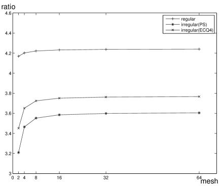
(b) Examle 3

Figure 5: The ratio $\eta_{r}/e_{r}$ for PS and ECQ4

References

• [1] I. Babu$\check{s}$ka, M. Suri, On locking and robustness in the finite element method, SIAM. J. Numer. Anal., 29: 1261-1293 (1992).
• [2] C. Bernardi, V. Girault, A local regularization operator for triangular and quadrilateral finite elements, SIAM. J. Numer. Anal., 35:1893-1916 (1998).
• [3] D. Braess, Enhanced assumed strain elements and locking in membrane problems, Comput. Meth. Appl. Mech. Energ., 165: 155-174 (1998).
• [4] D. Braess, C. Carstensen, and B. D. Reddy, Uniform convergence and a posteriori estimators for the enhanced strain finite element method, Numer. Math., 96: 461-479 (2004).
• [5] J. H. Bramble, R. D. Lazarov, J. E. Pasciak, Least-squares methods for linear elasticity based on a discrete minus one inner product, Comput. Meth. Appl. Mech. Energ., 191: 727-744 (2001).
• [6] F. Brezzi, On the existence, uniqueness and approximation of saddle-point problems arising from Lagrangian mulipliears, RAIRO Numer. Anal., 8-R2: 129-151 (1974).
• [7] F. Brezzi, M. Fortin, Mixed and hybrid finite element methods, Springer-Verlag, 1991.
• [8] C. Carstensen, A unifying theory of a posteriori finite element error control, Numer. Math., 100: 617-637(2005).
• [9] C. Carstensen, J. Hu, A. Orlando, Framework for the a posteriori error analysis of nonconforming finite elements. SIAM J Numer. Anal., 45: 68-82 (2007).
• [10] C. Carstensen, X.P. Xie, G.Z. Yu, T.X. Zhou, A priori and a posteriori analysis for a locking-free low order quadrilateral hybrid finite element for Reissner-Mindlin plates, Computer Methods in Applied Mechanics and Engineering (2010), doi: 10.1016/j.cma.2010.06.035.
• [11] P. G. Ciarlet, The Finite Element Method for Elliptic Problems. Amsterdam: North-Holland, 1978.
• [12] R. S. Falk, Nonconforming finite element methods for the equations of linear elasticity, Math. Comput., 57: 529-550 (1991).
• [13] B. P. Lamichhane, B. D. Reddy, B. Wohlmuth, Convergence in the incompressible limit of finite element approximations based on the Hu-Washizu formulation, Numer. Math., 104: 151-175 (2006).
• [14] P. Lesaint, On the convergence of Wilson’s nonconforming element for solving the elastic problem, Comput. Meth. Appl. Mech. Engrg. 7: 1-16 (1976).
• [15] P. Lesaint, M. Zl$\acute{a}$mal, Convergence of the nonconforming Wilson element for arbitrary quadrilateral meshes, Numer. Math., 36: 33-52 (1980).
• [16] T. H. H. Pian, Derivation of element stiffness matrices by assumed stress distributions, A.I.A.A.J., 2: 1333-1336 (1964).
• [17] T. H. H. Pian, D. P. Chen, Alternative ways of for formulation of hybrid stress elements, Int. J. Numer. Meths. Engng., 18: 1679-1684 (1982).
• [18] T. H. H. Pian, K. Sumihara, Rational approach for assumed stress finite element methods, Int. J. Numer. Meth. Engng., 20: 1685-1695 (1984).
• [19] T. H. H. Pian, C. C. Wu, A rational approach for choosing stress term of hybrid finite element formulations, Int. J. Numer. Meth. Engng., 26: 2331-2343 (1988).
• [20] T. H . H. Pian and Pin Tong, Relation between incompatible displacement model and hybrid stress model, Int. J. Numer. Meth Engng., 22: 173-182 (1989).
• [21] R. Piltner, R. L. Taylor, A quadrilateral mixed finite element with two enhanced strain modes. Int. J. Numer. Meth. Engng., 38: 1783-1808 (1995).
• [22] R. Piltner, R. L. Taylor, A systematic construction of B-bar functions for linear and non-linear mixed-enhanced finite elements for plane elasticity problem, Int. J. Numer. Meth. Engng., 44: 615-639 (1999).
• [23] R. Piltner, An alternative version of the Pian-Sumihara element with a simple extension to non-linear problems, Comput. Meth., 26: 483-489 (2000).
• [24] B. D. Reddy, J. C. Simo, Stability and convergence of a class of enhanced strain methods, SIAM J. Numer. Anal., 32: 1705-1728 (1995).
• [25] J. C. Simo, M. S. Rifai, A class of mixed assumed strain methods and the method of incompatible modes, Int. J. Numer. Meths. Engng., 29: 1595-1638 (1990).
• [26] Z. C. Shi, A convergence condition for the quadrilateral wilson element, Numer. Math., 44: 349-361 (1984).
• [27] R. L. Taylor, E. L. Wilson, P. J. Beresford, A nonconforming element for stress analysis, Int. J. Numer. Meth. Engng., 10: 1211-1219 (1976).
• [28] R. Verf$\ddot{\mbox{u}}$rth, A review of a posteriori error estimation and adaptive mesh-refinement Techniques, Wiley-Teubner, 1996.
• [29] E. L. Wilson, R. L. Taylor, W. P. Doherty, J. Ghaboussi, Incompatible displacement models, Numerical and Computer Methods in Structural Mechanics, New York: Academic Press Inc (1973).
• [30] X. P. Xie, T. X. Zhou, Optimization of stress modes by energy compatibility for 4-node hybrid quadrilaterals, Int. J. Numer. Meth. Engng., 59:293-313 (2004).
• [31] X. P. Xie, An accurate hybrid macro-element with linear displacements, Commun. Numer. Meth. Engng., 21:1-12 (2005).
• [32] X. P. Xie, T. X. Zhou, Accurate 4-node quadrilateral elements with a new version of energy-compatible stress mode, Commun. Numer. Meth. Engng., 24:125-139 (2008).
• [33] S. T. Yeo, B. C. Lee, Equivalence between enhanced assumed strain method and assumed stress hybrid method baded on the Hellinger-Reissner principle, Int. J. Numer. Meth. Engng., 39: 3083-3099 (1996).
• [34] Z. M. Zhang, Analysis of some quadrilateral nonconforming elements for incompressible elasticity, SIAM J. Numer. Anal., 34: 640–663 (1997).
• [35] T. X. Zhou, Y. F. Nie, Combined hybrid approach to finite element schemes of high performance, Int. J. Numer. Meth. Engng., 51: 181-202 (2001).
• [36] T. X. Zhou, X. P. Xie, A unified analysis for stress/strain hybrid methods of high performance, Comput. Meth. Appl. Mech. Eneng., 191: 4619-4640 (2002).