Nonparametric inference of doubly stochastic Poisson process data via the kernel method

Abstract

Doubly stochastic Poisson processes, also known as the Cox processes, frequently occur in various scientific fields. In this article, motivated primarily by analyzing Cox process data in biophysics, we propose a nonparametric kernel-based inference method. We conduct a detailed study, including an asymptotic analysis, of the proposed method, and provide guidelines for its practical use, introducing a fast and stable regression method for bandwidth selection. We apply our method to real photon arrival data from recent single-molecule biophysical experiments, investigating proteins’ conformational dynamics. Our result shows that conformational fluctuation is widely present in protein systems, and that the fluctuation covers a broad range of time scales, highlighting the dynamic and complex nature of proteins’ structure.

TX1Supported in part by the NSF Grant DMS-04-49204 and the NIH/NIGMS Grant 1R01GM090202-01.

and

1 Introduction

Poisson processes, fundamental to statistics and probability, have wide ranging applications in sciences and engineering. A special class of Poisson processes that researchers across different fields frequently encounter is the doubly stochastic Poisson process. Compared to the standard Poisson process, a key feature of a doubly stochastic one is that its arrival rate is also stochastic. In other words, if we let $N(t)$ denote the process and let $\lambda(t)$ denote the arrival rate, then, conditioning on $\lambda(t)$,

$$N(t)|\lambda(t)\sim\mbox{inhomogeneous Poisson process with rate }\lambda(t),$$

where $\lambda(t)$ itself is a stochastic process [Cox and Isham (1980); Daley and Vere-Jones (1988); Karr (1991); Karlin and Taylor (1981)]. In the literature such processes are also referred to as Cox processes in honor of their discoverer [Cox (1955a, 1955b)].

We consider the inference of Cox processes with large arrival rates in this article. Our study is primarily motivated by the frequent occurrences of Cox process data in biophysics and physical chemistry. In these fields, experimentalists commonly use fluorescence techniques to probe a biological system of interest [Krichevsky and Bonnet (2002)], where the system is placed under a laser beam, and the laser excites the system to emit photons. The experimental data consist of photon arrival times with the arrival rate depending on the stochastic dynamics of the system under study (for example, the active and inactive states of an enzyme can have different photon emission intensities). By analyzing the photon arrival data, one aims to learn the system’s biological properties, such as conformational dynamics and reaction rates.

Although we mainly focus on biophysical applications, we note that Cox processes also appear in other fields. In neuroscience Cox process data arise in the form of neural spike trains—a chain of action potentials emitted by a single neuron over a period of time [Gerstner and Kistler (2002)]—from which researchers seek to understand what information is conveyed in such a pattern of pulses, what code is used by neurons to transmit information, and how other neurons decode the signals, etc. [Bialek et al. (1991); Barbieri et al. (2005); Rieke et al. (1996)]. Astrophysics is another area where Cox process data often occur. For example, gamma-ray burst signals, pulsar arrival times and arrivals of high-energy photons [Meegan et al. (1992); Scargle (1998)] are studied to gain information about the position and motion of stars relative to the background [Carroll and Ostlie (2007)].

Previous statistical studies of Cox process data in the biophysics and chemistry literature mainly focus on constructing/analyzing parametric models. For instance, continuous-time Markov chains and stationary Gaussian processes have been used to model the arrival rate $\lambda(t)$ for enzymatic reactions [English et al. (2006); Kou et al. (2005b); Kou (2008b)], DNA dynamics [Kou, Xie and Liu (2005a)], and proteins’ conformational fluctuation [Min et al. (2005b); Kou and Xie (2004); Kou (2008a)].

Although effective for studying the stochastic dynamics of interest when they are correctly specified, parametric models are not always applicable for data analysis, especially when researchers (i) are in the early exploration of a new phenomenon, or (ii) are uncertain about the correctness of existing models, and try to avoid drawing erroneous conclusions from misspecified parametric models. Owing to its flexibility and the intuitive appeal of “learning directly” from data, we focus on the nonparametric inference of Cox process data in this paper. In particular, we develop kernel based estimators for the arrival rate $\lambda(t)$ and its autocorrelation function (ACF). The ACF is of interest because it directly measures the strength of dependence and reveals the internal structure of the system. For example, for biophysical data, a fast decay of the ACF, such as an exponential decay, indicates that the underlying biological process is Markovian and that the biomolecule under study has a relatively simple conformation dynamic, whereas a slow decay of ACF, such as a power-law decay, signifies a complicated process and points to an intricate internal structure/conformational dynamic of the biomolecule. Thus, in addition to discovering important characteristics of the stochastic dynamics under study, the autocorrelation function can also be used to test the validity of parametric models.

Kernel smoothing and density estimates have been extensively developed in the last three decades; see, for example, Silverman (1986), Eubank (1988), Müller (1998), Härdle (1990), Scott (1992), Wahba (1990), Wand and Jones (1994), Fan and Gijbels (1996) and Bowman and Azzalini (1997). Meanwhile, kernel estimators of spatial point processes motivated by applications in epidemiology, ecology and environment studies have been proposed; see Diggle (1985, 2003), Stoyan and Stoyan (1994), Moller and Waagepetersen (2003), Guan, Sherman and Calvin (2004, 2006) and Guan (2007). Compared to these spatial applications, the Cox processes that we encounter in biophysics have some unique features: (i) the arrival rates are usually large because strong light sources, such as laser, are often used; (ii) the data size tends to be large, since one can often control the experimental duration; (iii) both short-range and long-range dependent processes can govern the underlying arrival rate. Consequently, the estimators designed for spatial point processes are not always applicable to biophysical data. For example, the asymptotic variance formulas derived in the spatial context do not work for high intensity photon arrival data. The general cross-validation method for bandwidth selection [Guan (2007)], due to its intense computation, does not work well either for large photon arrival data. Furthermore, because of the large arrival rate, the statistical performance of the kernel estimate depends not only on the Poisson variation of $N(t)$ given $\lambda(t)$ but, more importantly, on the stochastic properties of $\lambda(t)$. For instance, we shall see in Section 4 that the kernel estimate of ACF will have asymptotically normal distribution only if $\lambda(t)$ has short-range dependence.

Similar to classical kernel estimation, there is a bandwidth selection problem associated with kernel inference of Cox process data. Using the mean integrated square error (MISE) criterion [Marron and Tsybakov (1995); Jones, Marron and Sheather (1996); Grund, Hall and Marron (1994); Marron and Wand (1992); Park and Turlach (1992); Diggle (2003)], we propose a stable and fast regression plug-in method to choose the bandwidth.

As our study is motivated by the analysis of scientific data, we apply our method to photon arrival data from real biophysical experiments. The result from our nonparametric inference helps elucidate the stochastic dynamics of proteins. In particular, our results show that as proteins (such as enzymes) spontaneously change their three-dimensional conformation, the conformational fluctuation covers a very broad range of time scales, highlighting the complexity of proteins’ conformational dynamics.

The rest of the paper is organized as follows. Section 2 considers kernel estimation of the arrival rate $\lambda(t)$. Section 3 focuses on estimating the ACF of $\lambda(t)$, and provides some guidelines for practical estimation. Section 4 investigates the asymptotic distribution of our kernel estimates, laying down the results for confidence interval construction. In Section 5 we apply our method to simulated data and photon arrival data from two biophysical experiments. We conclude in Section 6 with some discussion and future work. The technical proofs are provided in the supplementary material [Zhang and Kou (2010)].

2 Kernel estimation of the arrival rate

2.1 The estimator

Suppose within a time window $[0,T]$ a sequence of arrival times $s_{1},s_{2},\ldots,s_{K}$ has been observed from a Cox process $N(t)$, which has stochastic arrival rates $\lambda(t)$. The goal is to infer from the arrival times the stochastic properties of $\lambda(t)$. To do so, we assume the following:

Assumption 1.

The arrival rate $\lambda(t)$ is a stationary and ergodic process with finite fourth moments.

Stationarity (i.e., the distribution of $\{\lambda(t),t\in\mathsf{R}\}$ is time-shift invariant) and ergodicity (i.e., essentially $\frac{1}{T}\int_{0}^{T}\lambda(s)\,ds\rightarrow E[\lambda(0)]$, as $T\rightarrow\infty$) are both natural and necessary for making nonparametric inference of $\lambda(t)$ from a single sequence of arrival data. Assumption 1 is particularly relevant for single-molecule biophysical experiments [Kou (2009)] in which the system under study is typically in equilibrium or steady state.

With Assumption 1, we now construct a kernel based arrival rate estimator

$$\hat{\lambda}_{h}(t)=\sum_{i=1}^{K}f_{h}(t,s_{i}),\qquad\mbox{with }f_{h}(t,s)=\frac{1}{h}f\biggl{(}\frac{1}{h}(s-t)\biggr{)},$$ (1)

where $f$ is a symmetric density function, and $h$ is the bandwidth. When $f$ is taken to be the uniform kernel, $\hat{\lambda}_{h}(t)$ amounts to the binning-counting method used in the biophysics literature [Yang and Xie (2002a, 2002b)], in which $\lambda(t)$ is estimated by the number of data points falling into the bin containing $t$ divided by the bin width [see also Diggle (1985); Berman and Diggle (1989)]. One undesirable consequence of uniform kernel is that, as points move in and out of the bins, $\hat{\lambda}_{h}(t)$ is artificially discontinuous. We thus consider general $f$, and without loss of generality, we assume the following:

Assumption 2.

$f$ is a density function symmetric around 0 with bounded support $[-b,b]$.

The assumption of bounded support in fact can be relaxed—essentially all the results in this paper can be extended to kernels with unbounded supports. However, to make the theory more presentable and to reduce the length of algebra, we will work with Assumption 2.

When $t$ is getting too close to the boundaries of the observational time window $[0,T]$, there are apparently not enough data to estimate $\lambda(t)$ accurately. One method is to use end correction [see Diggle (1985); Berman and Diggle (1989)]: $\hat{\lambda}^{B}(t)=\sum_{i=1}^{k}f_{h}(t,s_{i})/\int_{0}^{T}f_{h}(t,s)\,ds$, which is identical to (1) if $t\in[bh,T-bh]$. However, the variance of the end-corrected-estimate $\hat{\lambda}^{B}(t)$ tends to be large when $t$ is close to $0$ or $T$. We, instead, estimate $\lambda(t)$ by

$$\hat{\lambda}_{h}(t)=\cases{\displaystyle{\sum_{i=1}^{K}f_{h}(t,s_{i})},&\quad if $bh\leq t\leq T-bh$,\cr\hat{\lambda}_{h}(bh),&\quad if $0\leq t<bh$,\cr\hat{\lambda}_{h}(T-bh),&\quad if $T-bh<t\leq T$,}$$ (2)

that is, we use $\hat{\lambda}_{h}(bh)$ and $\hat{\lambda}_{h}(T-bh)$ to approximate $\lambda(t)$ near the boundaries. We shall see shortly (Table 1) that for typical biophysical data the bandwidth $h$ is quite small; thus, the bias of (2) is also small.

Since the choice of the bandwidth $h$ affects the performance of the kernel estimate, we next determine the optimal $h$ that gives the smallest mean integrated square error (MISE)

$$\mathit{MISE}_{f}(h)=E\biggl{(}\frac{1}{T}\int_{0}^{T}\bigl{(}\hat{\lambda}_{h}(t)-\lambda(t)\bigr{)}^{2}\,dt\biggr{)}.$$

Owing to the stationarity and ergodicity of $\lambda(t)$, we have

$$\mathit{MISE}_{f}(h)=E\bigl{(}\hat{\lambda}_{h}(t_{0})-\lambda(t_{0})\bigr{)}^{2}+O(h/T),$$

where $t_{0}$ is any number within $[bh,T-bh]$, say, $t_{0}=T/2$, and the $O(h/T)$ term arises from the boundary of $[0,T]$. Hence, minimizing the MISE amounts to minimizing the MSE of $\hat{\lambda}_{h}(t_{0})$.

Let $C(t)$ denote the ACF of the arrival rate $\lambda(t)$: $C(t)=\operatorname{cov}(\lambda(0),\lambda(t))$. To find the optimal bandwidth that minimizes the MSE of $\hat{\lambda}_{h}(t_{0})$, we make one more assumption.

Assumption 3.

The ACF $C(t)$ is twice continuously differentiable for $t>0$, and has nonzero right derivative at 0, that is, $C^{\prime}(0^{+})=\lim_{s\rightarrow 0^{+}}(C(s)-C(0))/s$ exits and is nonzero.

This assumption reflects the fact that the arrival rate process $\lambda(t)$ in real experiments is usually not differentiable [Parzen (1962), Chapter 3]; for example, $\lambda(t)$ could be a finite-state continuous Markov chain, whose path consists of piecewise jumps and whose ACF is a mixture of exponential functions, which are nondifferentiable at zero, or $\lambda(t)$ could be a functional of a stationary nondifferentiable Gaussian process, such as the Ornstein–Uhlenbeck process (representing a harmonic oscillator).

Theorem 2.1.

Under Assumptions 1–3, the MSE of $\hat{\lambda}_{h}(t_{0})$ is given by

$$\qquad E\bigl{(}\hat{\lambda}_{h}(t_{0})-\lambda(t_{0})\bigr{)}^{2}=\frac{1}{h}E(\lambda(0))\int_{-b}^{b}f^{2}(r)\,dr+hC^{\prime}(0^{+})\gamma_{f}+R_{2}(h),$$ (3)

where the constant

$$\gamma_{f}=\int_{-b}^{b}\int_{-b}^{b}f(r_{1})f(r_{2})|r_{1}-r_{2}|\,dr_{1}\,dr_{2}-2\int_{-b}^{b}f(r)|r|\,dr<0,$$ (4)

and

$$R_{2}(h) = \int_{-b}^{b}\int_{-b}^{b}f(r_{1})f(r_{2})\int_{0}^{|r_{1}-r_{2}|h}(|r_{1}-r_{2}|h-s)C^{\prime\prime}(s)\,ds\,dr_{1}\,dr_{2}$$

$${}-2\int_{-b}^{b}f(r)\int_{0}^{|r|h}(|r|h-s)C^{\prime\prime}(s)\,ds\,dr=o(h).$$

The optimal $h$ that minimizes the sum of the first two terms (i.e., the main terms) of the right-hand side of (3) is given by

$$h_{\mathrm{opt}}=\biggl{[}\frac{E(\lambda(0))}{C^{\prime}(0^{+})\gamma_{f}}\int_{-b}^{b}f^{2}(r)\,dr\biggr{]}^{1/2}.$$ (5)

The constant $\gamma_{f}$ is strictly negative as long as $f$ is a density function. $R_{2}(h)$ is the remainder term. For data with large arrival rates, $h_{\mathrm{opt}}$ is small, and $R_{2}(h_{\mathrm{opt}})$ contributes little to the MSE. The proof of the theorem is given in the supplementary material [Zhang and Kou (2010)].

Since $h_{\mathrm{opt}}$ involves unknown quantities, for real applications we use a regression based plug-in method to estimate it. First, $\mu=E(\lambda(0))$ is unbiasedly estimated by $\hat{\mu}=K/T$, the total number of arrivals divided by the time window length, because

$$E(\hat{\mu})=\frac{1}{T}E\{E[k|\lambda(\cdot)]\}=\frac{1}{T}E\biggl{\{}\int_{0}^{T}\lambda(t)\,dt\biggr{\}}=E(\lambda(0)).$$

Next, we use a regression method to estimate $C^{\prime}(0^{+})$. We will discuss this regression estimate in detail in Section 3.2 when we study the ACF estimation. Plugging $\hat{\mu}$ and $\hat{C}^{\prime}(0^{+})$ into (5) yields our estimate $\hat{h}_{\mathrm{opt}}$.

2.2 Numerical illustration

We use two simulation examples to illustrate our method. In the first example, the arrival rate $\lambda(t)$ of the Cox process follows a continuous-time two-state Markov chain, which can be depicted as

$$A\mathop{\rightleftarrows}_{k_{2}}^{k_{1}}B,$$ (6)

where $k_{1}$ and $k_{2}$ represent the transition rates between the two states $A$ and $B$. This model has been used in the chemistry and biophysics literature [Reilly and Skinner (1994)] to model spectral and fluorescence data from two-level systems, such as the open-close of a DNA hairpin [Kou, Xie and Liu (2005a)], and the on-off of ion channels [Hawkes (2005); Sakmann and Neher (1995)]. We set the transition rates $k_{1}=2$, $k_{2}=5$ and arrival rates $\lambda_{A}=1000$ and $\lambda_{B}=400$ respectively at states $A$ and $B$ in the simulation; the observational time $T=500$. These numbers are taken to mimic a typical photon arrival experiment in biophysics. We generate a realization of $\lambda(t)$ from the two-state model and then the arrival times $s_{i}$, $i=1,\ldots,K$ on top of it. The true mean arrival rate $\mu=E(\lambda(0))=(k_{2}\lambda_{A}+k_{1}\lambda_{B})/(k_{1}+k_{2})$ is equal to $828.57$ in this case. The simulated data has the empirical mean arrival rate $\hat{\mu}=K/T=823.11$.

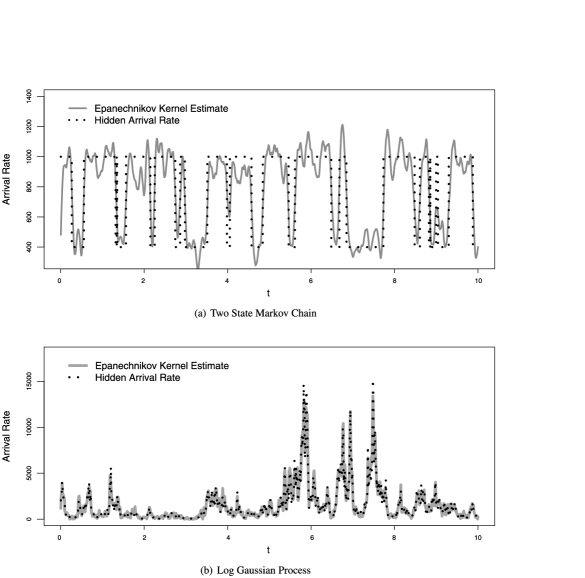
Figure 1: Arrival rate estimation. (a) Two state Markov chain with $\mu=828.57$ and $T=500$. (b) Log Gaussian $\lambda(t)$ with $\gamma(t)=1/(1+|t|)^{6}$ and $T=1500$.

Figure 1(a) shows the estimate $\hat{\lambda}_{\hat{h}_{\mathrm{opt}}}(t)$, compared with the true $\lambda(t)$, based on the Epanechnikov kernel $f(t)=\frac{3}{4}(1-t^{2})I(|t|\leq 1)$. Figure 1(a) represents a typical result. We see that $\lambda(t)$ is well recovered. Table 1 summarizes the results based on 100 independent simulations for applying our method with four different kernels: the uniform, Epanechnikov, triangular $f(t)=(1-|t|)I(|t|\leq 1)$ and quartic $f(t)=\frac{15}{16}(1-t^{2})^{2}I(|t|\leq 1)$ kernels. The second and third columns present the optimal bandwidth $h_{\mathrm{opt}}$ for each kernel and their estimates $\hat{h}_{\mathrm{opt}}$ obtained through the regression plug-in procedure. The next four columns show the normalized empirical MISE $\frac{1}{T\hat{\mu}^{2}}\int_{0}^{T}(\hat{\lambda}_{h}(t)-\lambda(t))^{2}\,dt$ for $h=h_{\mathrm{opt}}$, $\hat{h}_{\mathrm{opt}}$, $h_{\mathrm{opt}}/2$ and $2h_{\mathrm{opt}}$ respectively. It is noticeable that (i) the regression plug-in method for approximating $h_{\mathrm{opt}}$ works well; in particular, the empirical MISE with the estimated $\hat{h}_{\mathrm{opt}}$ is close to that of $h_{\mathrm{opt}}$; (ii) the performance of the kernel method largely depends on the choice of the bandwidth; if one uses a nonoptimal bandwidth, such as twice or half $h_{\mathrm{opt}}$, the error can increase as much as $30\%$; (iii) the choice of the kernel is not as crucial as that of the bandwidth, which echoes the classical result in kernel density estimation; and (iv) the widely used binning method, which is equivalent to using the uniform kernel, gives the largest error.

Table 1: Kernel estimates of the arrival rate for the two-state continuous-time Markov chain model. The second and third columns present the optimal bandwidth $h_{\mathrm{opt}}$ and the mean of their estimates $\hat{h}_{\mathrm{opt}}$ based on 100 simulations. The next several columns show the mean of the normalized empirical MISE $\frac{1}{T\hat{\mu}^{2}}\int_{0}^{T}(\hat{\lambda}_{h}(t)-\lambda(t))^{2}\ dt$ for $h=h_{\mathrm{opt}}$, $\hat{h}_{\mathrm{opt}}$, $h_{\mathrm{opt}}/2$ and $2h_{\mathrm{opt}}$ respectively. The numbers in the brackets are the associated standard deviations

	Bandwidth (in $\bolds{10^{-2}}$)		Normalized empirical MISE (in $\bolds{10^{-2}}$)
Kernel $\bolds{f}$	$\bolds{h_{\mathrm{opt}}}$	$\bolds{\hat{h}_{\mathrm{opt}}}$	$\bolds{h_{\mathrm{opt}}}$	$\bolds{\hat{h}_{\mathrm{opt}}}$	$\bolds{h_{\mathrm{opt}}/2}$	$\bolds{2h_{\mathrm{opt}}}$
Uniform	4.93	5.19 (0.34)	2.43 (0.057)	2.43 (0.059)	3.05 (0.050)	2.93 (0.092)
Epanechnikov	6.40	6.67 (0.50)	2.23 (0.053)	2.24 (0.055)	2.82 (0.048)	2.70 (0.085)
Quartic	7.74	8.07 (0.66)	2.20 (0.052)	2.21 (0.055)	2.78 (0.047)	2.65 (0.083)
Triangular	7.33	7.64 (0.63)	2.17 (0.052)	2.17 (0.054)	2.74 (0.047)	2.61 (0.082)

In the second example, the arrival rate $\lambda(t)$ follows a log Gaussian process: $\lambda(t)=M\exp(W(t))$, where $M>0$ and $W(t)$ is a stationary zero-mean Gaussian process with the autocovariance function $\gamma(t)$. It is straightforward to obtain $\mu=E(\lambda(t))=Me^{\gamma(0)/2}$ and $C(t)=M^{2}e^{\gamma(0)}(e^{\gamma(t)}-1)$. We take $\gamma(t)=1/(1+a|t|)^{H}$ so that $C(t)$ decreases at the order $t^{-H}$. Both $a$ and $H$ are positive constants. The log Gaussian process has been used to model the conformational dynamics and reactivity of enzyme molecules [Min et al. (2005a); Kou and Xie (2004)]. For instance, Kou and Xie (2004) showed that an enzyme’s conformational fluctuation can be modeled by a generalized Langevin equation, in which the $\lambda(t)$ follows a log Gaussian process with the ACF having a power law decay $C(t)\sim t^{-H}$. Here, we take $H=6$, $a=1$, $M=1000$ and $T=1500$ in our simulation to mimic a real photon arrival data of this kind. Figure 1(b) compares the estimate $\hat{\lambda}_{\hat{h}_{\mathrm{opt}}}(t)$ to the true $\lambda(t)$ for the Epanechnikov kernel. We repeat the simulation 100 times. Figure 1(b) represents a typical outcome. We see that $\lambda(t)$ is well recovered. The detailed estimation results are summarized in Table 2. Again, we can see that the regression plug-in method for estimating $h_{\mathrm{opt}}$ works well and that the performance of the kernel method depends largely on the choice of the bandwidth and less so on the kernels. The widely used binning method again gives the poorest result.

Table 2: Kernel estimates of the arrival rate for the log Gaussian model with $C(t)=1000^{2}\break\times(\exp(1/(1+|t|)^{6}+1)-e)$. The second and third columns present $h_{\mathrm{opt}}$ and the mean of the estimate $\hat{h}_{\mathrm{opt}}$ based on 100 simulations. The next four columns show the mean of the normalized empirical MISE for $h=h_{\mathrm{opt}}$, $\hat{h}_{\mathrm{opt}}$, $h_{\mathrm{opt}}/2$ and $2h_{\mathrm{opt}}$ respectively. The numbers in the brackets are the associated standard deviations

	Bandwidth (in $\bolds{10^{-3}}$)		Normalized empirical MISE (in $\bolds{10^{-2}}$)
Kernel $\bolds{f}$	$\bolds{h_{\mathrm{opt}}}$	$\bolds{\hat{h}_{\mathrm{opt}}}$	$\bolds{h_{\mathrm{opt}}}$	$\bolds{\hat{h}_{\mathrm{opt}}}$	$\bolds{h_{\mathrm{opt}}/2}$	$\bolds{2h_{\mathrm{opt}}}$
Uniform	$7.49$	$7.68\ (0.27)$	$8.08\ (0.16)$	$8.20\ (0.19)$	$10.3\ (0.17)$	$10.1\ (0.32)$
Epanechnikov	$9.73$	$10.1\ (0.28)$	$7.45\ (0.15)$	$7.45\ (0.15)$	$9.33\ (0.15)$	$9.26\ (0.30)$
Quartic	$11.8$	$12.1\ (0.32)$	$7.34\ (0.15)$	$7.34\ (0.15)$	$9.17\ (0.15)$	$9.14\ (0.29)$
Triangular	$11.1$	$11.4\ (0.30)$	$7.23\ (0.15)$	$7.23\ (0.15)$	$9.12\ (0.15)$	$8.97\ (0.29)$

3 Estimating the ACF

3.1 Kernel estimation

In this section we consider kernel estimation of the ACF $C(t)$ of the arrival rate. The ACF is useful in exploring the dependence structure of new stochastic dynamics and identifying appropriate parametric models for the data.

For example, most ion channel dynamics and most chemical reactions involve reversible transitions among the various discrete chemical states in which the system can exist. In these systems, a fast decay of the ACF, such as an exponential decay, indicates that the transition among the discrete states has a short memory, and the underlying biological process has a relatively simple mechanism, such as having only two or three states. In the case of ion channels, the simplest dynamic consists of a transition between a single shut state of the ion channel and a single open state [Sakmann and Neher (1995), Hawkes (2005)], in which the ACF is a single exponential function over time. In the case of a protein’s conformational fluctuation, the simplest scenario is a transition between two distinct conformation states (where the protein reversibly and spontaneously crosses the energy barrier that separates the two states). In the case of enzyme catalytic fluctuations, the simplest scenario is that the enzyme interconverts among a small numbers of states, in which the ACF has a near exponential decay [Schenter, Lu and Xie (1999); Yang and Xie (2002a, 2002b); Kou, Xie and Liu (2005a); Kou et al. (2005b)].

A slow decay of ACF, such as a power-law decay, on the other hand, signifies a complicated process and points to an intricate internal structure, such as the existence of a large number of conformation states or the presence of a complicated energy landscape [Kou and Xie (2004); Min et al. (2005b)].

To ease the presentation, we first consider the situation where the mean arrival rate $\mu=E(\lambda(0))$ is known, and later relax the results for unknown $\mu$. The basic idea is as follows. If we actually observe the realization of $\lambda(t)$, then using its ergodicity property, we have a natural estimate $\frac{1}{T-t}\int_{0}^{T-t}(\lambda(s)-\mu)(\lambda(s+t)-\mu)\,ds$ for $C(t)$. Now $\lambda(s)$ is unobserved; we replace it by $\hat{\lambda}_{h}(s)$. To avoid the bias at the boundary of the observation window, our kernel estimate of $C(t)$ is

$$\hat{C}_{\mu,h}(t)=\frac{1}{T-2bh-t}\int_{bh}^{T-bh-t}\bigl{(}\hat{\lambda}_{h}(s+t)-\mu\bigr{)}\bigl{(}\hat{\lambda}_{h}(s)-\mu\bigr{)}\,ds,$$

(7)

$$\eqntext{t\in[0,T-2bh).}$$ (8)

The next two lemmas tell us the bias and variance of $\hat{C}_{\mu,h}(t)$ for estimating $C(t)$ at a fixed $t$.

Lemma 3.1.

Under Assumptions 1 and 2,

$$E(\hat{C}_{\mu,h}(t)) = \frac{\mu}{h}\int_{-b}^{b}f\biggl{(}r+\frac{t}{h}\biggr{)}f(r)\,dr$$

$${}+\int_{-b}^{b}\int_{-b}^{b}C\bigl{(}|t+(r-m)h|\bigr{)}f(r)f(m)\,dr\,dm.$$

Furthermore, if Assumption 3 also holds, then

$$E(\hat{C}_{\mu,h}(t))$$

$$\qquad=\cases{\displaystyle C(t)+C^{\prime\prime}(t)h^{2}\int_{-b}^{b}r^{2}f(r)\,dr+o(h^{2}),&\quad$t\geq 2bh$;\cr\displaystyle{C(0)+\frac{\mu}{h}\int_{-b}^{b}f\biggl{(}r+\frac{t}{h}\biggr{)}f(r)\,dr}\cr\quad\displaystyle{}+C^{\prime}(0^{+})\int_{-b}^{b}\int_{-b}^{b}|t+(r-m)h|f(r)f(m)\,dr\,dm\cr\quad{}+o(h),&\quad$t\in[0,2bh)$.}$$

The bias of the ACF estimate $\hat{C}_{\mu,h}(t)$ is due to the fact that $\lambda(t)$ is estimated by “borrowing” information from the neighboring regions. When $t<2bh$, the data points used to calculate $\hat{\lambda}_{h}(s)$ and $\hat{\lambda}_{h}(s+t)$ overlap, resulting in the extra bias $\mu\int_{-b}^{b}f(r+t/h)f(r)\,dr/h.$

For notational convenience, we denote

$$C_{3}(t_{1},t_{2}) = E\bigl{\{}\bigl{(}\lambda(0)-\mu\bigr{)}\bigl{(}\lambda(t_{1})-\mu\bigr{)}\bigl{(}\lambda(t_{2})-\mu\bigr{)}\bigr{\}},$$

$$v(t_{1},t_{2},s^{\prime}-s) = \operatorname{cov}\bigl{\{}\bigl{(}\lambda(s)-\mu\bigr{)}\bigl{(}\lambda(s+t_{1})-\mu\bigr{)},\bigl{(}\lambda(s^{\prime})-\mu\bigr{)}\bigl{(}\lambda(s^{\prime}+t_{2})-\mu\bigr{)}\bigr{\}}.$$

Because of the stationarity of $\lambda(t)$, $C_{3}(t_{1},t_{2})=C_{3}(t_{2},t_{1})$ and $v(t_{1},t_{2},s^{\prime}-s)=v(t_{2},t_{1},s-s^{\prime})$. The following two technical assumptions are needed to characterize the asymptotic behavior of $\operatorname{var}(\hat{C}_{\mu,h}(t))$.

Assumption 4.

The three-step correlation $C_{3}(t_{1},t_{2})$ is continuous and satisfies

$$\lim_{|t_{2}|\rightarrow\infty}C_{3}(t_{1},t_{2})=0\qquad\mbox{for any fixed }t_{1}.$$

Assumption 5.

The cross correlation $v(t_{1},t_{2},s)$ is continuous and satisfies

$$\lim_{|s|\rightarrow\infty}v(t_{1},t_{2},s)=0\qquad\mbox{for any fixed }t_{1}\mbox{ and }t_{2}.$$

These two assumptions reflect the intuitive idea that as time-points move far away from each other, their dependence should eventually vanish. They are satisfied by most stationary and ergodic processes that one encounters in practice, such as continuous-time finite-state Markov Chains and functionals of stationary and ergodic Gaussian processes.

Lemma 3.2.

The variance of $\hat{C}_{\mu,h}(t)$ can be decomposed as

$$\operatorname{var}(\hat{C}_{\mu,h}(t))=\operatorname{var}\{E(\hat{C}_{\mu,h}(t)|\lambda(\cdot))\}+E\{\operatorname{var}(\hat{C}_{\mu,h}(t)|\lambda(\cdot))\}.$$ (10)

Under Assumptions 1, 2, 4 and 5,

$$\operatorname{var}\{E(\hat{C}_{\mu,h}(t)|\lambda(\cdot))\}$$

$$\qquad=\frac{1}{(T-2bh-t)^{2}}\biggl{(}A_{t,T}^{h}+\frac{2}{h}B_{t,T}^{h}+\frac{1}{h^{2}}C_{t,T}^{h}\biggr{)}\rightarrow 0,\qquad\mbox{as }T\rightarrow\infty,$$

where

$$A_{t,T}^{h}=\int\!\!\!\int_{[bh,T-bh-t]^{2}}\biggl{[}\int\!\!\!\int\!\!\!\int\!\!\!\int_{[-b,b]^{4}}v\bigl{(}t+(l-m)h,t+(l^{\prime}-m^{\prime})h,$$

$$\hskip 63.0pt\hphantom{A_{t,T}^{h}=\int\!\!\!\int_{[bh,T-bh-t]^{2}}\biggl{[}\int\!\!\!\int\!\!\!\int\!\!\!\int_{[-b,b]^{4}}}s^{\prime}-s+(l^{\prime}-l)h\bigr{)}f(l)$$

$$\hskip 6.0pt\hphantom{A_{t,T}^{h}=\int\!\!\!\int_{[bh,T-bh-t]^{2}}\biggl{[}\int\!\!\!\int\!\!\!\int\!\!\!\int_{[-b,b]^{4}}}{}\times f(m)f(l^{\prime})f(m^{\prime})\ dl\ dm\ dl^{\prime}\ dm^{\prime}\biggr{]}\ ds\ ds^{\prime},$$

$$B_{t,T}^{h}=\int\!\!\!\int_{[bh,T-bh-t]^{2}}\biggl{[}\int\!\!\!\int\!\!\!\int\!\!\!\int_{[-b,b]^{3}}C_{3}\bigl{(}t+(l^{\prime}-m^{\prime})h,$$

$$\hphantom{B_{t,T}^{h}=\int\!\!\!\int_{[bh,T-bh-t]^{2}}\biggl{[}\int\!\!\!\int\!\!\!\int\!\!\!\int_{[-b,b]^{3}}C_{3}\bigl{(}}s-s^{\prime}+t+(l-m^{\prime})h\bigr{)}f(l^{\prime})$$

$$\hphantom{B_{t,T}^{h}=\int\!\!\!\int_{[bh,T-bh-t]^{2}}\biggl{[}\int\!\!\!\int\!\!\!\int\!\!\!\int_{[-b,b]^{3}}C_{3}\bigl{(}}\times f(m^{\prime})f(l)f\biggl{(}l+\frac{t}{h}\biggr{)}\ dl\ dm^{\prime}\ dl^{\prime}\biggr{]}\ ds\ ds^{\prime},$$

$$C_{t,T}^{h}=\int\!\!\!\int_{[bh,T-bh-t]^{2}}\biggl{[}\int\!\!\!\int_{[-b,b]^{2}}C\bigl{(}s^{\prime}-s+(l^{\prime}-l)h\bigr{)}f(l)$$

$$\hphantom{C_{t,T}^{h}=\int\!\!\!\int_{[bh,T-bh-t]^{2}}\biggl{[}\int\!\!\!\int_{[-b,b]^{2}}}{}\times f\biggl{(}l+\frac{t}{h}\biggr{)}f(l^{\prime})f\biggl{(}l^{\prime}+\frac{t}{h}\biggr{)}\ dl\ dl^{\prime}\biggr{]}\ ds\ ds^{\prime},$$

and

$$\qquad E\{\operatorname{var}(\hat{C}_{\mu,h}(t)|\lambda(\cdot))\}=\frac{1}{T-2bh-t}\biggl{(}D_{t}^{h}+\frac{1}{h}E_{t}^{h}+\frac{1}{h^{2}}F_{t}^{h}\biggr{)}+O\biggl{(}\frac{h}{T^{2}}\biggr{)},$$ (12)

where the three terms $D_{t}^{h},E_{t}^{h}$ and $F_{t}^{h}$ do not depend on $T$. Their exact but lengthy expressions, involving multiple integrals, are given in the supplementary material [Zhang and Kou (2010)].

Equation (10) indicates that the variance of the ACF estimate arises from two sources: the Poisson variation—$E\{\operatorname{var}(\hat{C}_{\mu,h}(t)|\lambda(\cdot))\}$—and the variation from $\lambda(t)$ – $\mathrm{var}\{E(\hat{C}_{\mu,h}(t)|\lambda(\cdot))\}$. $A_{t,T}^{h}$ is the main part of $\mathrm{var}\{E(\hat{C}_{\mu,h}(t)|\lambda(\cdot))\}$. When $t>2bh$, $B_{t,T}^{h}$ and $C_{t,T}^{h}$ both equal zero.

Based on Lemmas 3.1 and 3.2, the next theorem tells us that as the observation time $T$ gets larger, $\hat{C}_{\mu,h}(t)$ consistently estimates $C(t)$.

Theorem 3.3.

Suppose that $C(t)$ is a continuous function of $t\in[0,\infty)$ and that Assumptions 1, 2, 4 and 5 hold. Then for any fixed $t>0$, as $T\cdot h\rightarrow\infty$ and $h\rightarrow 0$,

$$\hat{C}_{\mu,h}(t)\rightarrow C(t)\qquad\mbox{in }L^{2},$$

so, in particular,

$$\hat{C}_{\mu,h}(t)\rightarrow C(t)\qquad\mbox{in probability}.$$

The assumption of continuous $C(t)$ is satisfied for general continuous-time stationary and ergodic processes. We note that in the context of spatial point processes, different estimates of the covariance function have been proposed [see, e.g., Stoyan and Stoyan (1994) and Diggle (2003)]. We use (3.1) here mainly due to its internal coherency: an estimate of $\lambda(t)$ naturally leads to an estimate of $C(t)$.

3.2 Practical consideration

To use the kernel estimate in practice, a few issues arise naturally.

Unknown $\mu$

In real applications, the mean arrival rate $\mu$ is unknown. Employing its unbiased estimate $\hat{\mu}=K/T$, we use

$$\hat{C}_{\hat{\mu},h}(t)=\frac{1}{T-2bh-t}\int_{bh}^{T-bh-t}\bigl{(}\hat{\lambda}_{h}(s+t)-\hat{\mu}\bigr{)}\bigl{(}\hat{\lambda}_{h}(s)-\hat{\mu}\bigr{)}\,ds$$

to estimate the ACF. A question follows immediately: is $\hat{C}_{\hat{\mu},h}(t)$ still a consistent estimator? The next theorem provides a positive answer.

Theorem 3.4.

Suppose that $C(t)$ is a continuous function of $t\in[0,\infty)$ and that Assumptions 1, 2, 4 and 5 hold. Then for any fixed $t>0$, as $T\cdot h\rightarrow\infty$ and $h\rightarrow 0$,

$$\hat{C}_{\hat{\mu},h}(t)\rightarrow C(t)\qquad\mbox{in probability}.$$

Bias correction for small $t$

From Lemma 3.1, we see that $\hat{C}_{\mu,h}(t)$ has an extra bias $\mu\int_{-b}^{b}f(r+t/h)f(r)\,dr/h$ for $t<2bh$. A bias correction can be conducted for $t<2bh$, yielding

$$\tilde{C}_{\hat{\mu},h}(t)=\hat{C}_{\hat{\mu},h}(t)-\frac{\hat{\mu}}{h}\int_{-b}^{b}f\biggl{(}r+\frac{t}{h}\biggr{)}f(r)\,dr.$$ (13)

Estimating $h_{\mathrm{opt}}$

In Section 2 we briefly described how to estimate $h_{\mathrm{opt}}$ to recover the arrival rate, where the key is to estimate the derivative $C^{\prime}(0^{+})$. With Lemma 3.1 established, we now explain our estimate in detail. Lemma 3.1 tells us that, for small $t$, the expectation of $\tilde{C}_{\hat{\mu},h}(t)$ depends on $\int_{-b}^{b}\int_{-b}^{b}|t+(r-m)h|f(r)f(m)\,dr\,dm$ linearly with $C^{\prime}(0^{+})$ as the slope. This suggests that we can calculate $Y_{i}=\tilde{C}_{\hat{\mu},h}(t_{i})$ for evenly spaced $t_{i}\in[0,2bh)$, say, ten points, and regress $Y_{i}$ on $X_{i}=\int_{-b}^{b}\int_{-b}^{b}|t_{i}+(r-m)h|f(r)f(m)\,dr\,dm$. The regression slope is our estimate of $C^{\prime}(0^{+})$. Compared to the naive idea of using a numerical derivative $(\hat{C}(\Delta)-\hat{C}(0))/\Delta$ for some small $\Delta$ to approximate $C^{\prime}(0^{+})$, this regression estimate is not only easy to implement, but, more importantly, much stabler in performance (see Figure 2).

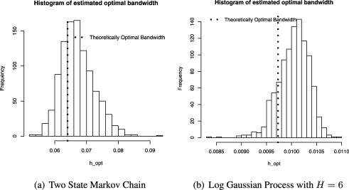
Figure 2: Estimating the optimal bandwidth with the Epanechnikov kernel.

For the calculation of $\tilde{C}_{\hat{\mu},h}(t_{i})$, one needs to start from an initial $h$. We use $h=\rho/\hat{\mu}=\rho T/K$, where the constant $\rho$ (for example, between 3 and 10) is the average number of data points falling in an interval of length $h$. This choice of initial $h$ ensures that there are enough points in the kernel to give reliable $\tilde{C}_{\hat{\mu},h}(t_{i})$. Throughout our simulation and real data analysis, where $\hat{\mu}$ is in the hundreds, we found that taking $\rho$ between 3 and 10 gives almost identical results. Figure 2 shows how our estimate $\hat{h}_{\mathrm{opt}}$ behaves for the two simulation examples of Section 2: the two-state Markov chain and the log Gaussian process model. The dotted vertical line is the true $h_{\mathrm{opt}}$. The histograms in Figure 2 are based on 1000 i.i.d. replications of the Cox process. The estimate $\hat{h}_{\mathrm{opt}}$ is seen to be stable and close to $h_{\mathrm{opt}}$.

The bandwidth $h$ for estimating $C(t)$

To estimate the ACF $C(t)$, a natural question is the choice of $h$. It could be different from that associated with recovering the arrival rate. One approach might be as follows: based on the results of Lemmas 3.1 and 3.2, find the asymptotic leading terms in bias-square and variance, and then search for $h$ to optimize their linear combination. Although conceptually “simple”, this approach in fact has several major difficulties that make it ineffective for practical use: (a) As the equations in Lemmas 3.1 and 3.2 involve fourth moment and covariance of $\lambda(t)$, one needs to estimate them. Since the estimates of high moments often have large variability, the resulting $h$ tends to be highly variable. (b) The bias and variance formulas depend on the specific value of $t$, which implies that for each $t$ there is an $h$. Consequently, if the entire curve $C(t)$ is of interest (as in many scientific studies), the computation becomes very intensive. (c) In order for the bias-squared to become comparable to the variance and in order for the asymptotics to take effect, $h$ needs to be much smaller than $(C(t)+\mu^{2})/(\int_{0}^{T}v(t,t,s)\,ds)$, which in turn requires $T$ to be quite large: $T\sim O((C(t)+\mu^{2})/(C^{\prime\prime}(t)^{2}h^{5}))$. However, real biophysical data with large $\mu$ and moderate $T$ hardly satisfy this requirement. (d) In order to identify the asymptotic leading terms, more technical assumptions, such as short-range dependence of $\lambda(t)$ [i.e., $\int_{0}^{\infty}C(t)\,dt<\infty$], have to be imposed, which restricts the estimate’s general applicability.

For these reasons, we recommend using $\hat{h}_{\mathrm{opt}}$ for $t\geq 2b\hat{h}_{\mathrm{opt}}$ and a smaller bandwidth $h=\min(\rho/\hat{\mu},\hat{h}_{\mathrm{opt}})$, where $\rho\in[3,10]$ for $t<2b\hat{h}_{\mathrm{opt}}$ to estimate the ACF $C(t)$. The reason to use $\min(\rho/\hat{\mu},\hat{h}_{\mathrm{opt}})$ instead of $\hat{h}_{\mathrm{opt}}$ for $t<2b\hat{h}_{\mathrm{opt}}$ is that for large mean arrival rate $\mu$, $\rho/\hat{\mu}$ can be smaller than $\hat{h}_{\mathrm{opt}}$; in this case Lemma 3.1 tells us that for small $t$ the bias of $\tilde{C}_{\hat{\mu},h}(t)$ from $h=\rho/\hat{\mu}$ tends to be smaller than that of $\hat{h}_{\mathrm{opt}}$, while Lemma 3.2 indicates that the variances of the two are about the same. Thus, for small $t$, $\min(\rho/\hat{\mu},\hat{h}_{\mathrm{opt}})$ appears to be a better choice. Although our bandwidth recommendation does not guarantee the smallest MSE for $C(t)$ at every $t$, it does offer a stable and easy-to-compute bandwidth. We will demonstrate the effectiveness of this choice in Section 5 (see Table 3) when we study confidence interval construction.

Approximating the variance of $\hat{C}_{\mu,h}(t)$

For estimating the variance of $\hat{C}_{\mu,h}(t)$ (e.g., in confidence interval construction), one can in principle use Lemma 3.2, replacing the unknown quantities with their empirical counterparts. However, this approach does not work well for the real data that we have tried for two reasons: (a) Multiple integrals on empirical third or higher moments tend to be highly variable. (b) The computing demands are quite high given the many multiple integrals involved. Fortunately, we find an efficient shortcut. First, when the mean arrival rate $\mu$ is large, variation from the underlying stochastic arrival rate dominates in the variance decomposition (10): $\operatorname{var}\{E(\hat{C}_{\mu,h}(t)|\lambda(\cdot))\}\gg E\{\operatorname{var}(\hat{C}_{\mu,h}(t)|\lambda(\cdot))\}$. Proposition 3.5 below gives a theoretical justification. Second, for the real biophysical experimental data that we have tried, $\operatorname{var}\{E(\hat{C}_{\mu,h}(t)|\lambda(\cdot))\}$ accounts for more than 95% of the total variance $\operatorname{var}(\hat{C}_{\mu,h}(t))$. Furthermore, in these real data, $A_{t,T}^{h}/(T-2bh-t)^{2}$ in the decomposition (3.2) of $\operatorname{var}\{E(\hat{C}_{\mu,h}(t)|\lambda(\cdot))\}$ provides more than 90% of $\operatorname{var}(\hat{C}_{\mu,h}(t))$. These observations suggest that we can use $A_{t,T}^{h}/(T-2bh-t)^{2}$ to approximate $\operatorname{var}(\hat{C}_{\mu,h}(t))$.

Proposition 3.5.

Denote $\lambda_{0}(t)=\lambda(t)/\mu$, that is, $E(\lambda_{0}(t))=1$ and $\lambda(t)=\mu\lambda_{0}(t)$. Suppose the law of $\{\lambda_{0}(t),t\in\mathsf{R}\}$ is fixed. Then under Assumptions 1–3, for any fixed $T$, $h$ and $t$,

$$\frac{A_{t,T}^{h}}{(T-2bh-t)^{2}}\big{/}\operatorname{var}(\hat{C}_{\mu,h}(t))\rightarrow 1,\qquad\mbox{as }\mu\rightarrow\infty,$$ (14)

where $A_{t,T}^{h}$ is defined in Lemma 3.2.

This proposition directly relates to real experimental data, especially those from fluorescence biophysical experiments. In such experiments the samples are usually placed under a laser beam, and the photon arrival intensity is proportional to the laser strength. To illuminate the sample, experimenters usually use a strong laser. In this scenario, since the intrinsic molecular dynamics do not change, the law of $\{\lambda_{0}(t)\}$ remains the same, while $\mu$ is large.

The approximation of $A_{t,T}^{h}/(T-2bh-t)^{2}$ can be further simplified for practical use. First, because the bandwidth $h$ is usually chosen to be small, and $v(\cdot,\cdot,\cdot)$ is a continuous function, $A_{t,T}^{h}$ approximately equals $\int\int_{[bh,T-bh-t]^{2}}\*v(t,t,s^{\prime}-s)\,ds\,ds^{\prime}$. Second, since the process $\{\lambda(s),s\in\mathsf{R}\}$ is stationary, and to accurately estimate $C(t)$, $t$ is usually small compared to $T$ (in order to have enough data), $\int\int_{[bh,T-bh-t]^{2}}v(t,t,s^{\prime}-s)\,ds\,ds^{\prime}$ approximately equals $\frac{2}{(T-2bh-t)^{2}}\!\int_{0}^{T-t-2bh}(T-t-r)v(t,t,r)\,dr$. Third, replacing

$$v(t,t,r)=E\bigl{(}\bigl{(}\lambda(0)-\mu\bigr{)}\bigl{(}\lambda(t)-\mu\bigr{)}\bigl{(}\lambda(r)-\mu\bigr{)}\bigl{(}\lambda(r+t)-\mu\bigr{)}\bigr{)}-C^{2}(t)$$

with its empirical counterpart $\operatorname{\hat{cov}}(t,r)$, which is

$$\operatorname{\hat{cov}}(t,r)=\max\biggl{\{}\frac{1}{T-2bh-r-t}$$

$$\hphantom{\operatorname{\hat{cov}}(t,r)=\max\biggl{\{}}{}\times\int_{bh}^{T-bh-r-t}\bigl{(}\hat{\lambda}_{h}(s)-\hat{\mu}\bigr{)}\bigl{(}\hat{\lambda}_{h}(s+t)-\hat{\mu}\bigr{)}\bigl{(}\hat{\lambda}_{h}(r+s)-\hat{\mu}\bigr{)}$$

$$\hskip 21.0pt\hphantom{\hat{cov}(t,r)=\max\biggl{\{}{}\times\int_{bh}^{T-bh-r-t}}{}\times\bigl{(}\hat{\lambda}_{h}(r+s+t)-\hat{\mu}\bigr{)}\,ds-\hat{C}_{\hat{\mu},h}^{2}(t),0\biggr{\}},$$

results in the final approximation of $\operatorname{var}(\hat{C}_{\mu,h}(t))$:

$$\hat{V}(t)=\frac{2}{(T-2bh-t)^{2}}\int_{0}^{T-t-2bh}(T-t-2bh-r)\operatorname{\hat{cov}}(t,r)\ dr.$$ (15)

Note that $v(t,t,r)$ is typically nonnegative, so we force $\operatorname{\hat{cov}}(t,r)$ to be nonnegative also. We will demonstrate the use of $\hat{V}(t)$ in Section 5.

Comparison with existing methods

Diggle (1985) provided a procedure for selecting the bandwidth for estimating the arrival rate $\lambda(t)$ in the case of $f$ being the uniform kernel. In this procedure, based on an estimate $\widehat{\mathit{MSE}}(h)$ of $E(\hat{\lambda}_{h}(t)-\lambda(t))^{2},$ the bandwidth is chosen to be the one that gives the smallest $\widehat{\mathit{MSE}}(h)$. Figure 3(a) shows the standardized estimate $\widehat{\mathit{MSE}}(h)/\hat{\mu}^{2}$ for the data of Figure 1(a) by this approach. However, this method is computationally more intensive than our method, since it involves estimating MSE for all the possible bandwidths. Moreover, the MSE estimator provided by Diggle (1985) is only meant for the uniform kernel and does not generalize to other kernels.

Figure 3: (a) $\widehat{\operatorname{MSE}}(h)$ vs. bandwidth using Diggle’s (1985) method for data from the two-state model. (b) The bandwidth selected by the subsampling procedure. The histogram is based on 100 i.i.d. replications of the Cox process from the two-state model.

Guan (2007) has proposed a composite likelihood cross-validation approach in selecting bandwidth for estimating the ACF. However, due to the large data size in our study (more than two million arrival points), this method is computationally too expensive to use (we found that the C program cannot even finish in an affordable time).

We also applied the subsampling procedure of Guan, Sherman and Calvin (2004, 2006) to our data. Figure 3(b) shows the histogram of the bandwidths selected by the subsampling procedure based on 100 i.i.d. simulations from the two-state model in Section 2. We found that this procedure leads to a much larger bandwidth than $\hat{h}_{\mathrm{opt}}$ proposed in Section 2, and, consequently, the estimates of $C(t)$ have large bias, particularly for $t$ close to zero.

Compared to the existing methods, in terms of computational effort, our proposed method takes no more than five minutes to finish analyzing a process with more than two million data points, including estimating the arrival rate and the autocorrelation function and constructing the confidence intervals.

Connection with the classical kernel density estimate

Despite its similarity with the classical kernel density estimate, the kernel estimates $\hat{\lambda}_{h}(t)$ and $\hat{C}_{\mu,h}(t)$ have several distinct features: (i) Since $\lambda(t)$ is stochastic, a consistent estimate of $\lambda(t)$ does not exist. (ii) In classical kernel problems, the number of observations $K$ does not depend on the underlying density, whereas the total number of observations in our case is random and depends on the stochastic process $\{\lambda(t),t\in[0,T]\}$. Consequently, (iii) consistency refers to the observational window $T\rightarrow\infty$. (iv) The asymptotic behavior of the kernel estimate would depend on the distributional properties of $\lambda(t)$, as we shall see next.

4 Asymptotic distribution of the kernel estimate

We investigate the limiting behavior of the kernel estimate $\hat{C}_{\mu,h}(t)$ in this section, since the asymptotic normality plays an important role in confidence interval construction. For well-behaved $\lambda(t)$, we can show that the asymptotic normality of $\hat{C}_{\mu,h}(t)$ holds.

$\rho$-mixing arrival rate

Let $\mathcal{F}_{t}=\sigma(\lambda(s)\dvtx s\leq t)$ be the sigma field generated by $\lambda(s)$ for $s\leq t$, and $\mathcal{G}_{t}=\sigma(\lambda(s)\dvtx s\geq t)$ be the tail sigma field generated by $\lambda(s)$ for $s\geq t$. Define

$$\qquad\rho_{t}=\sup\{E(\xi\eta)\dvtx\xi\in\mathcal{F}_{s},E\xi=0,\|\xi\|\leq 1;\eta\in\mathcal{G}_{s+t},E\eta=0,\|\eta\|\leq 1\}.$$ (16)

$\lambda(t)$ is said to be finite $\rho$-mixing if $\int_{0}^{\infty}\rho_{s}\,ds<\infty$ [Billingsley (1999)].

Theorem 4.1.

Suppose that Assumptions 1, 2, 4 and 5 hold, and that the arrival rate process $\{\lambda(t),t\in\mathsf{R}\}$ is bounded and finite $\rho$-mixing. Then for fixed $t,h\geq 0$,

$$\sqrt{T}[\hat{C}_{\mu,h}(t)-E(\hat{C}_{\mu,h}(t))]\stackrel{{\scriptstyle D}}{{\rightarrow}}N(0,\sigma^{2}(t,h))\qquad\mbox{as }T\rightarrow\infty,$$ (17)

where $\sigma^{2}(t,h)=\lim_{T\rightarrow\infty}T\operatorname{var}(\hat{C}_{\mu,h}(t))$.

Theorem 4.2.

Suppose that Assumptions 1 and 2 hold and that the stochastic process $\lambda(s)$ is a continuous-time Markov chain with finite number of states. Then for fixed $t,h\geq 0$, the asymptotic normality (17) holds with $\sigma^{2}(t,h)=\lim_{T\rightarrow\infty}T\operatorname{var}(\hat{C}_{\mu,h}(t))$.

Theorem 4.2 covers a large class of arrival rates. Another class of processes, widely used in the physical science literature, is functionals of stationary Gaussian processes: $\lambda(s)=g(W(s))$, where $g$ is a positive and continuous function, and $\{W(s),s\in\mathsf{R}\}$ is a zero-mean Gaussian process. We will see that as long as the autocorrelation of $W(s)$ decays reasonably fast, the asymptotic normality of $\hat{C}_{\mu,h}(t)$ remains true.

We consider, in particular, Gaussian processes of the form

$$\qquad\bigl{\{}W(t),t\in\mathsf{R}\dvtx W(t)=W(j\varepsilon)\mbox{ for }t\in\bigl{[}j\varepsilon,(j+1)\varepsilon\bigr{)},j=0,\pm 1,\pm 2,\ldots\bigr{\}},$$ (18)

where $\varepsilon>0$ is a fixed constant. In other words, we consider Gaussian processes generated piecewise by a discrete skeleton: $\{\ldots,W(-2\varepsilon),W(-\varepsilon),\break W(0),W(\varepsilon),W(2\varepsilon),\ldots\}$, where $W(j\varepsilon)$ is a discrete-time stationary zero-mean Gaussian process. The reason that we focus on this type of Gaussian process is two fold: first, if $\varepsilon$ is small enough, $W$ can essentially approximate any continuous stationary Gaussian process with arbitrary precision, and this is typically how one simulates a Gaussian process; second, the theoretical calculations behind continuous-time Gaussian processes, especially those regarding mixing conditions, are quite delicate [see, e.g., Ibragimov and Rozanov (1978)], so to avoid drifting too much into the mathematical details and to present our proofs in a concise manner, we work on (18). We have the following result on functionals of Gaussian processes; its proof is given in the supplementary material [Zhang and Kou (2010)].

Theorem 4.3.

Suppose that Assumptions 1, 2, 4 and 5 hold, and that $\lambda(s)=g(W(s))$, where $g$ is a positive and bounded measurable function, and $\{W(s),s\in\mathsf{R}\}$, defined in (18), is generated from a discrete skeleton $\{W(j\varepsilon)\}$. If the ACF $\gamma(j\varepsilon)=\operatorname{cov}(W(0),W(j\varepsilon))$ satisfies $\sum_{j=0}^{\infty}|\gamma(j\varepsilon)|<\infty$, then for any fixed $t$ and $h$, the asymptotic normality (17) of $\hat{C}_{\mu,h}(t)$ holds with $\sigma^{2}(t,h)=\lim_{T\rightarrow\infty}T\operatorname{var}(\hat{C}_{\mu,h}(t))$.

Long-range dependent processes

Stochastic processes with a finite integrated correlation $\int_{0}^{\infty}C(t)\,dt<\infty$ are said to be short-range dependent. Our results essentially say that for Cox processes with short-range dependent arrival rates, we expect the asymptotic normality of $\hat{C}_{\mu,h}(t)$ to hold, which offers a big advantage in the confidence interval construction. For long-range dependent arrival rates ($\int_{0}^{\infty}C(t)\,dt=\infty$), however, no easy conclusion can be drawn about the asymptotic behavior of $\hat{C}_{\mu,h}(t)$. Even the form of limiting law varies from case to case. For example, the limiting process might be a fractional Brownian Motion [Whitt (2002)], a stable L$\mathrm{\acute{e}}$vy motion [Whitt (2002)] or a Rosenblatt process [Taqqu (1975)]. Moreover, the variance of the limiting law, most likely, will not be the same as the limit of the variance [Taqqu (1975)], that is, $\lim_{T\rightarrow\infty}\operatorname{var}(\hat{C}_{\mu,h}(t)/\sqrt{\operatorname{var}(\hat{C}_{\mu,h}(t))})\neq\operatorname{var}(\lim_{T\rightarrow\infty}\hat{C}_{\mu,h}(t)/\sqrt{\operatorname{var}(\hat{C}_{\mu,h}(t))})$. Therefore, an interesting open problem is to investigate the asymptotic behavior of the Cox process estimates with long-range dependent arrival rates.

5 Numerical study of ACF estimation

We illustrate our method through several numerical examples—both simulation and real biophysical experimental data. We use the Epanechnikov kernel throughout this section.

5.1 Simulation examples

Finite-state Markov chains

Since Theorem 4.2 guarantees the asymptotic normality of the kernel ACF estimate, we can construct a pointwise $1-\alpha$ approximate confidence interval (C.I.) of $C(t)$ via

$$\biggl{[}\tilde{C}_{\hat{\mu},h}(t)-\Phi^{-1}\biggl{(}1-\frac{\alpha}{2}\biggr{)}\sqrt{\hat{V}(t)},\tilde{C}_{\hat{\mu},h}(t)+\Phi^{-1}\biggl{(}1-\frac{\alpha}{2}\biggr{)}\sqrt{\hat{V}(t)}\biggr{]},$$ (19)

where $\tilde{C}_{\hat{\mu},h}(t)$ and $\hat{V}(t)$ are given in (13) and (3.2) respectively. Following the discussion in Section 3.2, we use $h=\min(5/\hat{\mu},\hat{h}_{\mathrm{opt}})$ for $t<2b\hat{h}_{\mathrm{opt}}$ and $h=\hat{h}_{\mathrm{opt}}$ for $t\geq 2b\hat{h}_{\mathrm{opt}}$.

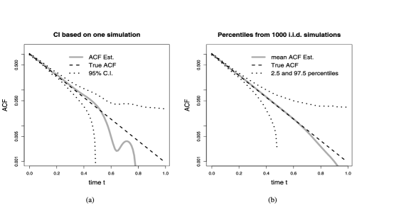
Figure 4: ACF estimation for two-state Markov chains. The left panel shows $\tilde{C}_{\hat{\mu},h}(t)$ (the time $t$ is in second) and the approximate 95% C.I. [normalized by $\tilde{C}_{\hat{\mu},h}(0)$] based on one sequence of arrival data. The right panel shows the 2.5 and 97.5 percentiles of $\tilde{C}_{\hat{\mu},h}(t)$ calculated from 1000 i.i.d. repetitions from the same model.

We revisit the two-state Markov chain model (6) in Section 2. In this case, the true ACF is exponential: $C(t)=(\lambda_{A}-\lambda_{B})^{2}k_{1}k_{2}\exp(-(k_{1}+k_{2})t)/\break(k_{1}+k_{2})^{2}$. We applied the kernel estimator and (19) to the data set simulated in Section 2 [Figure 1(a)]. Figure 4(a) shows $\tilde{C}_{\hat{\mu},h}(t)$ as the solid line, and the point-wise 95% C.I. as the dotted lines. The true ACF $C(t)$, shown as the dashed line, is well recovered. Since $C(t)$ usually decays quite fast, to highlight the details, especially around the tails, we plotted the estimate on the logarithm scale. We see from Figure 4(a) that $\log\tilde{C}_{\hat{\mu},h}(t)$ is linear with $t$, indicating the exponential decay of $C(t)$. As a check for the accuracy of the C.I., we repeated the data generation 1000 times independently. For each simulated data set, we calculated $\tilde{C}_{\hat{\mu},h}(t)$. The 2.5 and 97.5 percentiles of these repeated estimates $\tilde{C}_{\hat{\mu},h}(t)$ give the real 95% coverage of $\tilde{C}_{\hat{\mu},h}(t)$, which is shown on Figure 4(b). Comparing the two panels, we see that the variance estimate based on just one realization is close to the truth. From the 1000 i.i.d. repetitions, we calculated the coverage probabilities of the 95% C.I. (19) for various $t$. Table 3 (the second row) reports the numbers, which are close to the nominal 95%; Figure 5(a) plots them graphically.

Table 3: The coverage probabilities of the 95% C.I. (19) at various time points for different models based on 1000 i.i.d. repetitions. For reference, the standard deviation of a binomial proportion with success probability of 0.95 and 1000 trails is 0.0069

	Time $\bolds{t}$
Coverage probability	0.01	0.02	0.05	0.1	0.2	0.5	1	2	5	10
Two state	0.97	0.97	0.97	0.96	0.93	0.97	0.97	0.96	0.97	0.96
Log-Gaussian $H=6$	0.91	0.92	0.92	0.93	0.93	0.94	0.95	0.97	0.95	0.96
Log-Gaussian $H=0.5$	0.57	0.58	0.59	0.60	0.62	0.63	0.66	0.66	0.65	0.66

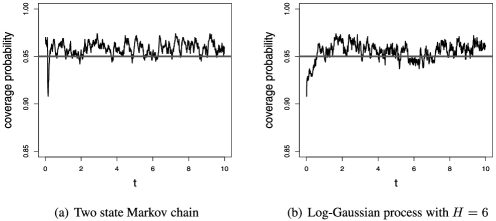
Figure 5: The coverage probabilities of the 95% C.I. (19) for $t\in[0,10]$ (the time $t$ is in second) under different models.

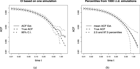
Figure 6: ACF estimation for a short-range dependent log-Gaussian process with $C(t)=10^{6}(\exp(1/(1+|t|)^{6}+1)-e)$ (the time $t$ is in second). The left panel shows $\tilde{C}_{\hat{\mu},h}(t)$ and the approximate 95% C.I. [normalized by $\tilde{C}_{\hat{\mu},h}(0)$] based on one sequence of arrival data. The right panel shows the 2.5 and 97.5 percentiles of $\tilde{C}_{\hat{\mu},h}(t)$ calculated from 1000 i.i.d. replications from the same model. The total observational time $T$ equals $1500$. Both graphs are plotted on the log–log scale.

Log Gaussian processes

We next consider examples where the arrival rate $\lambda(t)$ follows a log Gaussian process: $\lambda(t)=M\exp\{W(t)\}$, where $W(t)$ is a stationary zero-mean Gaussian process with the ACF $\gamma(t)$. As we mentioned in Section 2, the log Gaussian process has been used to model the conformational dynamics and reactivity of enzyme molecules [Min et al. (2005a); Kou and Xie (2004)]. As in Section 2, we take $\gamma(t)=1/(1+a|t|)^{H}$ so that $C(t)=M^{2}(\exp(\gamma(t)+1)-e)$ decreases at the order of $t^{-H}$. Both $a$ and $H$ are positive constants. The larger the decay slope $H$, the faster the $C(t)$ converges to zero and the faster the estimate converges to $C(t)$. $H$ also determines the dependence structure of the Cox process: if $H\leq 1$, the process is long-range dependent. In the simulation, we generate $W(t)$ through the discrete skeleton (18), and then draw the arrival times $s_{1},s_{2},\ldots$ on top of $\lambda(t)$. For each simulated arrival sequence, we calculate the kernel estimate $\tilde{C}_{\hat{\mu},h}(t)$ and the 95% C.I. (19).

We consider two log Gaussian processes: one with $H=6$ and $a=1$, and the other with $H=0.5$ and $a=20$. In both cases, the maximum observational time $T=1500$ and the constant $M$ is taken to be $1000$ to mimic typical photon arrival data from a biophysical experiment. For the log Gaussian process with $H=6$, Figure 6(a) plots $\tilde{C}_{\hat{\mu},h}(t)$ and the 95% approximate C.I. based on one data set. Figure 6(b) plots the 2.5 and 97.5 percentiles of $\tilde{C}_{\hat{\mu},h}(t)$ from 1000 i.i.d. repetitions. For easy visual detection of the power law decay, the graph is plotted on a log–log scale. The similarity between the left and right panels indicates the effectiveness of our method. The real coverage probabilities of the 95% C.I. (19) are shown in Figure 5(b) and Table 3 (the third row). We see that the real coverage probabilities for the $H=6$ case are close to the nominal 95%. Figure 6 also suggests that $\log C(t)$ is roughly linear with $\log t$ near the tail of the curve.

The log Gaussian process with $H=0.5$ and $a=20$ is long-range dependent. We can still calculate $\tilde{C}_{\hat{\mu},h}(t)$ and the C.I. (19). However, since even asymptotic normality is no longer valid, one would expect the real coverage to be way off. Figure 7 contrasts the “C.I.” based on one data set with the true 2.5 and 97.5 percentiles of $\tilde{C}_{\hat{\mu},h}(t)$ from 1000 i.i.d. replications. It is evident that although $\tilde{C}_{\hat{\mu},h}(t)$ still estimates $C(t)$ reasonably well, the “C.I.” constructed from one data set is quite narrower than the true percentiles. The last row of Table 3 shows that the real coverage probabilities of (19) in this long-range dependent case are much smaller than the nominal 95%—clearly the asymptotic variance is underestimated.

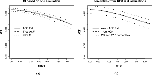
Figure 7: ACF estimation for a long-range dependent log-Gaussian process with $C(t)=10^{6}(\exp(1/(1+20|t|)^{0.5}+1)-e)$ (the time $t$ is in second). The left panel shows $\tilde{C}_{\hat{\mu},h}(t)$ and the approximate 95% C.I. [normalized by $\tilde{C}_{\hat{\mu},h}(0)$] based on one sequence of arrival data. The right panel shows the 2.5 and 97.5 percentiles of $\tilde{C}_{\hat{\mu},h}(t)$ calculated from 1000 i.i.d. replications from the same model. The total observational time $T$ equals $1500$. Both graphs are plotted on the log–log scale.

Static processes

Our method can be easily applied to detect static processes. When the underlying biological process is static, the photon arrival rate $\lambda(t)$ is a constant, and $C(t)\equiv 0$ for $t>0$. In this case, we would observe that the arrival rate estimate $\hat{\lambda}_{\hat{h}_{\mathrm{opt}}}(t)$ oscillates around a constant, and the ACF estimate $\tilde{C}_{\hat{\mu},h}(t)$ clusters around zero. Figure 8 shows such an example with constant arrival rate $\lambda(t)\equiv 500$ and $T=500$.

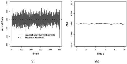
Figure 8: Analyzing Cox process data with constant arrival rate $\lambda(t)\equiv 500$ and $T=500$. (a) Arrival rate estimate. (b) ACF estimate (normalized by $\hat{\mu}^{2}$).

5.2 Experimental photon arrival data

Studying the conformational dynamics of proteins is of current biophysical interest. For example, scientists have become aware that an enzyme’s conformational fluctuation can directly affect its catalytic activity—certain conformations yield highly active catalysis, whereas others lead to less active catalysis [Lu, Xun and Xie (1998); English et al. (2006)]. A recent single-molecule experiment [Yang et al. (2003)] investigates the conformational dynamics of a protein-enzyme compound Fre, which is involved in the DNA synthesis of E. Coli. In the experiment, the protein compound is immobilized and placed under a laser beam. Photons from the laser-excited molecule are collected. Since the photon arrival rate depends on the molecule’s time-varying three-dimensional conformation (different conformations of Fre generate different arrival rates), the spontaneous conformation fluctuation of Fre leads to a stochastic arrival rate. The ACF of the photon arrival rates therefore reflects the time dependence of Fre’s conformational fluctuation [Weiss (2000)].

The experimental photon arrival data has a total observational time $T=354$ seconds. The empirical mean arrival rate $\hat{\mu}=534.6$ counts/second. We first estimated the arrival rate and showed it in Figure 9(a). This plot leads to a natural question regarding the nature of Fre’s conformational fluctuation: does Fre have a small number of distinct conformation states or many? Looking at the decay of $C(t)$ provides one way to address this question. We applied the bias-corrected $\tilde{C}_{\hat{\mu},h}(t)$ to estimate $C(t)$. Figure 9(b) shows $\tilde{C}_{\hat{\mu},,h}(t)$ and its approximate 95% C.I. (19). We plotted the estimates on a log–log scale to give a better view of the decay of the ACF. The apparent linear pattern suggests a power-law relationship. If there are only two, three or even four conformation states, then $C(t)$ should be a mixture of no more than three exponential functions. The apparent power-law relationship indicates a different picture: instead of having two, three or even four discrete conformation states, the 3D conformation of Fre appears to fluctuate over a continuum (as a check, we have attempted to parametrically fit a mixture of three exponentials to the estimated ACF, but even the best fitting is very poor), so the parametric finite state Markov Chain model cannot be applied here. The slow decay of the ACF thus points to a complicated conformation dynamic of Fre, which implies that the enzyme’s catalytic rate could vary over a broad range, a phenomenon called dynamic disorder in the biophysics literature [Min et al. (2005a); Lerch, Rigler and Mikhailov (2005)].

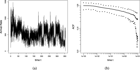
Figure 9: Analyzing the photon arrival data from a single-molecule experiment with $T=354.3$ and $\hat{\mu}=534.6$. (a) Arrival rate estimate. (b) ACF estimate and its 95% confidence interval plotted on the log–log scale.

Another recent single-molecule experiment [Min et al. (2005b)] also investigates protein’s conformational dynamics, studying a protein complex formed by fluorescein and monoclonal antifluorescein. This protein complex is an antibody-antigen system. Like the previous compound, the 3D conformation of the molecule spontaneously fluctuates over time. To study the conformational dynamics, the immobilized protein complex was placed under a laser beam. Photons from the laser-excited molecule are collected. The photon arrival rate $\lambda(t)$ depends on the molecule’s time-varying conformation. Figure 10(a) shows the arrival rate estimates for this data, which have $T=1312.8$ and $\hat{\mu}=1523.5$. This plot seems to suggest that there are many conformation states in this antibody-antigen system. To further investigate, we applied $\tilde{C}_{\hat{\mu},h}(t)$ to estimate $C(t)$. Figure 10(b) shows our estimate and the approximate 95% C.I. (19) on a log–log scale. Again, we observed a slow decay of the ACF. We attempted to parametrically fit a mixture of three exponentials to the estimated ACF but only obtained a very poor result. Like the previous system, it appears that the 3D conformation of this antibody-antigen system fluctuates over a broad range rather than over just a few, say, three of four, discrete states.

Figure 10: Analyzing the photon arrival data from another single-molecule experiment with $T=1312.8$ and $\hat{\mu}=1523.5$. (a) Arrival rate estimate. (b) ACF estimate and its 95% confidence interval plotted on the log–log scale.

Since the second experiment is on a totally different system from the first, our statistical results indicate that (i) conformational fluctuation could be widely present in protein systems; (ii) the fluctuation appears to be over a broad range of time scales. Our results thus support the growing understanding in the biophysics community that proteins’ conformational fluctuation is a complex phenomenon, which in turn affects some crucial functions of proteins, such as enzyme catalysis [Lerch, Rigler and Mikhailov (2005); English et al. (2006)] and electron transfer in photosynthesis [Wang et al. (2007)].

6 Conclusion

Motivated by the analysis of experimental data from biophysics, we propose a nonparametric kernel based method for inferring Cox process in this article, complementing existing parametric approaches. An important feature of the arrival data in biophysics is that the arrival rate is often large, which makes the methods developed for analyzing spatial point processes (which usually have low arrival rates), such as variance estimate, bandwidth selection and asymptotic theory, not directly applicable for our purpose. In addition to proposing the kernel estimates, we conduct a detailed study of their properties. We show that the asymptotic normality of our ACF estimates holds for most short-range dependent processes, which provides the theoretical underpinning for confidence interval construction. We provide an approximation of the variance of the ACF estimate, which accounts for at least 90% of the total variation in our examples. We can possibly improve this approximation, for example, by taking into account the Poisson variation $E\{\operatorname{var}(\hat{C}_{\mu,h}(t)|\lambda(\cdot))\}$ part, which might be particularly beneficial when $\lambda(t)$ has a strong short-range dependence.

We applied our nonparametric method to analyze two real photon arrival data produced in recent (single-molecule) biophysical experiments. Using our kernel ACF estimate, we examine the conformational dynamics of two different protein systems. We observed that the conformational fluctuation exhibits a long memory and spans a broad range of time scales, confirming the recent experimental discovery that the classical static picture of proteins that researchers used to assume needs to be revised.

An important open question for future study is to investigate Cox processes with long-range dependent arrival rates. Another open question for our future investigation is the estimation of high-order correlations of the arrival rate, as biophysicists and chemists have used them to discriminate different mechanistic and phenomenological models [Mukamel (1995)].

Acknowledgments. The authors are grateful to the Xie group at the Department of Chemistry and Chemical Biology of Harvard University for sharing the experimental data. We also thank Yongtao Guan, the editor, the associate editor and the referees for helpful suggestions.

[id=suppA] Technical proofs [doi]10.1214/10-AOAS352SUPP [url]http://lib.stat.cmu.edu/aoas/352/supplement.pdf .pdf Technical proofs accompanying the paper “Nonparametric inference of doubly stochastic Poisson process data via the kernel method” by Zhang and Kou.

References

- Barbieri et al. (2005) Barbieri, R., Wilson, M. A., Frank, L. M. and Brown, E. N. (2005). An analysis of hippocampal spatio-temporal representations using a Bayesian algorithm for neural spike train decoding. IEEE Transactions on Neural Systems and Rehabilitation Engineering 13 131–136.
- Berman and Diggle (1989) Berman, M. and Diggle, P. J. (1989). Estimating weighted integrals of the second-order intensity of a spatial point process. J. Roy. Statit. Soc. Ser. B 51 81–92. \MR0984995
- Bialek et al. (1991) Bialek, W., Rieke, F., Steveninck, R. and Warland, D. (1991). Reading a neural code. Science 252 1854–1857.
- Billingsley (1999) Billingsley, P. (1999). Convergence of Probability Measures, 2nd ed. Wiley, New York. \MR1700749
- Bowman and Azzalini (1997) Bowman, A. and Azzalini, A. (1997). Applied Smoothing Techniques for Data Analysis: The Kernel Approach With S-PLUS Illustrations. Oxford Univ. Press, New York.
- Carroll and Ostlie (2007) Carroll, B. and Ostlie, D. (2007). An Introduction to Modern Astrophysics, 2nd ed. Benjamin Cummings, Reading, MA.
- Cox (1955a) Cox, D. R. (1955a). The analysis of non-Markovian stochastic processes by the inclusion of supplementary variables. Proc. Camb. Phil. Soc. 51 433–441. \MR0070093
- Cox (1955b) Cox, D. R. (1955b). Some statistical methods connected with series of events. J. R. Statist. Soc. Ser. B 17 129–164. \MR0092301
- Cox and Isham (1980) Cox, D. R. and Isham, V. (1980). Point Processes. Chapman and Hall, London. \MR0598033
- Daley and Vere-Jones (1988) Daley, D. J. and Vere-Jones, D. (1988). An Introduction to the Theory of Point Processes. Springer, New York. \MR0950166
- Diggle (1985) Diggle, P. (1985). A kernel method for smoothing point process data. Appl. Statist. 34 138–147.
- Diggle (2003) Diggle, P. (2003). Statistical Analysis of Spatial Point Patterns. Oxford Univ. Press, New York. \MR0743593
- English et al. (2006) English, B., Min, W., van Oijen, A. M., Lee, K. T., Luo, G., Sun, H., Cherayil, B. J., Kou, S. C. and Xie, X. S. (2006). Ever-fluctuating single enzyme molecules: Michaelis–Menten equation revisited. Nature Chem. Biol. 2 87–94.
- Eubank (1988) Eubank, R. L. (1988). Nonparametric Regression and Spline Smoothing. Marcel Dekker, New York. \MR1680784
- Fan and Gijbels (1996) Fan, J. and Gijbels, I. (1996). Local Polynomial Modelling and Its Applications. Chapman and Hall, London. \MR1383587
- Gerstner and Kistler (2002) Gerstner, W. and Kistler, W. (2002). Spiking Neuron Models: Single Neurons, Populations, Plasticity. Cambridge Univ. Press. \MR1923120
- Grund, Hall and Marron (1994) Grund, B., Hall, P. and Marron, J. S. (1994). Loss and risk in smoothing parameter selection. Nonparametr. Stat. 4 133–147. \MR1290924
- Guan (2007) Guan, Y. (2007). A composite likelihood cross-validation approach in selecting bandwidth for the estimation of the pair Correlation function. Scand. Statist. 34 336–346. \MR2346643
- Guan, Sherman and Calvin (2004) Guan, Y., Sherman, M. and Calvin, J. A. (2004). A nonparametric test for spatial isotropy using subsampling. J. Amer. Statist. Assoc. 99 810–821. \MR2090914
- Guan, Sherman and Calvin (2006) Guan, Y., Sherman, M. and Calvin, J. A. (2006). Assessing isotropy for spatial point processes. Biometrics 62 126–134. \MR2226565
- Härdle (1990) Härdle, W. (1990). Applied Nonparametric Regression. Cambridge Univ. Press. \MR1161622
- Hawkes (2005) Hawkes, A. G. (2005). Ion channel modeling. In Encyclopedia of Biostatistics, 2nd ed. (P. Armitage and T. Colton, eds.) 4 2625–2632. Wiley, Chichester.
- Ibragimov and Rozanov (1978) Ibragimov, I. A. and Rozanov, Y. A. (1978). Gaussian Random Processes. New York, Springer. \MR0543837
- Jones, Marron and Sheather (1996) Jones, M. C., Marron, J. S. and Sheather, S. J. (1996). A brief survey of bandwidth selection for density estimation. J. Amer. Statist. Assoc. 91 401–407. \MR1394097
- Karlin and Taylor (1981) Karlin, S. and Taylor, H. M. (1981). A Second Course in Stochastic Processes. Academic Press, New York. \MR0611513
- Karr (1991) Karr, A. F. (1991). Point Processes and Their Statistical Inference, 2nd ed. Marcel Dekker, New York. \MR1113698
- Kou (2008a) Kou, S. C. (2008a). Stochastic modeling in nanoscale biophysics: Subdiffusion within proteins. Ann. Appl. Statist. 2 501–535. \MR2524344
- Kou (2008b) Kou, S. C. (2008b). Stochastic networks in nanoscale biophysics: Modeling enzymatic reaction of a single protein. J. Amer. Statist. Assoc. 103 961–975. \MR2462886
- Kou (2009) Kou, S. C. (2009). A selective view of stochastic inference and modeling problems in nanoscale biophysics. Science in China A 52 1181–1211. \MR2520569
- Kou et al. (2005b) Kou, S. C., Cherayil, B., Min, W., English, B. and Xie, X. S. (2005b). Single-molecule Michaelis–Menten equations. J. Phys. Chem. B 109 19068–19081.
- Kou and Xie (2004) Kou, S. C. and Xie, X. S. (2004). Generalized Langevin equation with fractional Gaussian noise: Subdiffusion within a single protein molecule. Phys. Rev. Lett. 93 180603(1)–180603(4).
- Kou, Xie and Liu (2005a) Kou, S. C., Xie, X. S. and Liu, J. S. (2005a). Bayesian analysis of single-molecule experimental data (with discussion) J. Roy. Statist. Soc. Ser. C 54 469–506. \MR2137252
- Krichevsky and Bonnet (2002) Krichevsky, O. and Bonnet, G. (2002). Fluorescence correlation spectroscopy: The technique and its applications. Report on Progress in Physics 65 251–297.
- Lerch, Rigler and Mikhailov (2005) Lerch, H., Rigler, R. and Mikhailov, A. (2005). Functional conformational motions in the turnover cycle of cholesterol oxidase. Proc. Natl. Acad. Sci. USA 102 10807–10812.
- Lu, Xun and Xie (1998) Lu, H. P., Xun, L. and Xie, X. S. (1998). Single-molecule enzymatic dynamics. Science 282 1877–1882.
- Marron and Tsybakov (1995) Marron, J. S. and Tsybakov, A. B. (1995). Visual error criteria for qualitative smoothing. J. Amer. Statist. Assoc. 90 499–507. \MR1340502
- Marron and Wand (1992) Marron, J. S. and Wand, M. P. (1992). Exact mean integrated squared error. Ann. Statist. 20 712–736. \MR1165589
- Meegan et al. (1992) Meegan, C. A., Fishman, G. J., Wilson, R. B., Paciesas, W. S., Pendleton, G. N., Horack, J. M., Brock, M. N. and Kouveliotou, C. (1992). Spatial distribution of gamma ray bursts observed by BATSE. Nature 355 142–145.
- Min et al. (2005a) Min, W., English, B., Luo, G., Cherayil, B., Kou, S. C. and Xie, X. S. (2005a). Fluctuating enzymes: Lessons from single-molecule studies. Accounts of Chemical Research 38 923–931.
- Min et al. (2005b) Min, W., Luo, G., Cherayil, B., Kou, S. C. and Xie, X. S. (2005b). Observation of a power law memory kernel for fluctuations within a single protein molecule. Phys. Rev. Lett. 94 198302(1)–198302(4).
- Moller and Waagepetersen (2003) Moller, J. and Waagepetersen, R. P. (2003). Statistical Inference and Simulation for Spatial Point Processes. Chapman and Hall, New York. \MR2004226
- Mukamel (1995) Mukamel, S. (1995). Principle of Nonlinear Optical Spectroscopy. Oxford Univ. Press.
- Müller (1998) Müller, H. G. (1988). Nonparametric Regression Analysis of Longitudinal Data. Springer, New York. \MR0960887
- Park and Turlach (1992) Park, B. U. and Turlach, B. A. (1992). Practical performances of several data-driven bandwidth selectors (with discussion). Comput. Statist. 7 251–285.
- Parzen (1962) Parzen, E. (1962). Stochastic Processes. Holden Day, Inc., San Francisco, CA. \MR0139192
- Reilly and Skinner (1994) Reilly, P. D. and Skinner, J. L. (1994). Spectroscopy of a chromophore coupled to a lattice of dynamic two-level systems. J. Chem. Phys. 101 959–973.
- Rieke et al. (1996) Rieke, F., Warland, D., de Ruyter van Steveninck, R. and Bialek, W. (1996). Spikes: Exploring the Neural Code. MIT Press, Cambridge, MA. \MR1983010
- Sakmann and Neher (1995) Sakmann, B. and Neher, E. (1995). Single Channel Recording, 2nd ed. Plenum Press, New York.
- Scargle (1998) Scargle, J. D. (1998). Studies in astronomical time series analysis. V. Bayesian blocks, a new method to analyze structure in photon counting data. Astrophys. J. 504 405–418.
- Schenter, Lu and Xie (1999) Schenter, G. K., Lu, H. P. and Xie, X. S. (1999). Statistical analyses and theoretical models of single-molecule enzymatic dynamics. J. Phys. Chem. A 103 10477–10488.
- Scott (1992) Scott, D. W. (1992). Multivariate Density Estimation: Theory, Practice, and Visualization. Wiley, New York. \MR1191168
- Silverman (1986) Silverman, B. W. (1986). Density Estimation for Statistics and Data Analysis. Chapman and Hall, London. \MR0848134
- Stoyan and Stoyan (1994) Stoyan, D. and Stoyan, H. (1994). Fractals, Random Shapes and Point Fields. Wiley, New York. \MR1297125
- Taqqu (1975) Taqqu, M. S. (1975). Weak convergence to fractional Brownian motion and to the Rosenblatt process, Z. Wahrsch. verw. Gebiete 31 287–302. \MR0400329
- Wahba (1990) Wahba, G. (1990). Spline Models for Observational Data. SIAM, Philadelphia. \MR1045442
- Wand and Jones (1994) Wand, M. P. and Jones, M. C. (1994). Kernel Smoothing. Chapman and Hall, London. \MR1319818
- Wang et al. (2007) Wang, H., Lin, S., Allen, J. P., Williams, J. C., Blankert, S., Laser C. and Woodbury, N. W. (2007). Protein dynamics control the kinetics of initial electron transfer in photosynthesis. Science 316 747–750.
- Weiss (2000) Weiss, S. (2000). Measuring conformational dynamics of biomolecules by single molecule fluorescence spectroscopy. Nature Struct. Biol. 7 724–729.
- Whitt (2002) Whitt, W. (2002). Stochastic-Process Limits. Springer, New York. \MR1876437
- Yang and Xie (2002a) Yang, H. and Xie, X. S. (2002a). Statistical approaches for probing single-molecule dynamics photon by photon. Chem. Phys. 284 423–437.
- Yang and Xie (2002b) Yang, H. and Xie, X. S. (2002b). Probing single molecule dynamics photon by photon. J. Chem. Phys. 117 10965–10979.
- Yang et al. (2003) Yang, H., Luo, G., Karnchanaphanurach, P., Louise, T.-M., Rech, I., Cova, S., Xun, L. and Xie, X. S. (2003). Protein conformational dynamics probed by single-molecule electron transfer. Science 302 262–266.
- Zhang and Kou (2010) Zhang, T. and Kou, S. C. (2010). Supplement to “Nonparametric inference of doubly stochastic Poisson process data via the kernel method.” DOI: 10.1214/10-AOAS352SUPP.