Compton Upconversion of Twisted Photons:
Backscattering of Particles with Non-Planar Wave Functions

Abstract

Twisted photons are not plane waves, but superpositions of plane waves with a defined projection $\hbar m$ of the orbital angular momentum onto the propagation axis ($m$ is integer and may attain values $m\gg 1$). Here, we describe in detail the possibility to produce high-energy twisted photons by backward Compton scattering of twisted laser photons on ultra-relativistic electrons with a Lorentz-factor $\gamma=E/(m_{e}c^{2})\gg 1$. When a twisted laser photon with the energy $\hbar\omega\sim 1\,{\rm eV}$ performs a collision with an electron and scatters backward, the final twisted photon conserves the angular momentum $m$, but its energy $\hbar\omega^{\prime}$ is increased considerably: $\omega^{\prime}/\omega=4\gamma^{2}/(1+x)$, where $x=4E\,\hbar\omega/(m_{e}\,c^{2})^{2}$. The $S$ matrix formalism for the description of scattering processes is particularly simple for plane waves with definite 4-momenta. However, in the considered case, this formalism must be enhanced because the quantum state of twisted particles cannot be reduced to plane waves. This implies that the usual notion of a cross section is inapplicable, and we introduce and calculate an averaged cross section for a quantitative description of the process. The energetic upconversion of twisted photons may be of interest for experiments with the excitation and disintegration of atoms and nuclei, and for studying the photo-effect and pair production off nuclei in previously unexplored regimes.
PACS 12.20.-m, 12.20.Ds, 13.60.Fz, 42.50.-p, 42.65.Ky

1 Introduction

Scattering processes lie at the heart of modern physics and have been studied in detail at the tree- and loop-level for particles with well-defined four momenta. In particular, the well-known Feynman rules of quantum electrodynamics BeLiPi1982vol4 ; ItZu1980 apply to the scattering of planar waves and cannot be readily applied to the scattering of particles with more complex wave functions. Consequently, the literature is more scarce when it comes to the scattering of quantal particles described by non-planar waves.

The related questions are far from being academic. E.g., a description using non-planar waves is necessary in the case of single photon bremsstrahlung discovered in experiments on the $e^{+}e^{-}$ collider VEPP-4 BlEtAl1982 ; BaKaSt1982 ; BuDeMisc and then on the $ep$ collider HERA Pi1995 . In these experiments, a remarkable deviation of the measured bremsstrahlung photons from standard calculational methods has been observed. The decrease in the number of observed photons can be explained by the fact that large impact parameters (of the two bunches relative to each other) give the essential contributions to the cross section. These parameters are larger by several orders of magnitude than the transverse beam size. In that case, the standard definitions for the cross section and the number of events become invalid. In particular, it is possible to calculate the $S$ matrix element as a superposition of “planar” scattering processes, but the normalization of the flux of incoming particles still constitutes a problem in the calculation of the modified cross section (beyond the $S$ matrix element). Modified calculational schemes for the description of particle production in the interaction of two bunches have to be employed (for details, see the review KoSeSc1992 ). In this scheme, the colliding bunches are represented as wave packets, and quantum distribution functions are used. The modified definitions of the cross section and the number of events contain the features of “non–locality” and “interference.”

An analogous problem is studied here for Compton backscattering of so-called “twisted photons.” These are defined superpositions of plane waves and have some interesting physical properties FAAlPa1992 ; PaCoAl2004 , such as wavefronts that rotate about the propagation axis and Poynting vectors that look like corkscrews (see Fig. 1 of Ref. MaVaWeZe2001 ). Also, twisted photons have a defined projection of the orbital angular momentum $\hbar m$ onto the propagation axis Gr2003 ; FAAlPa2008 which may be quite large, $m\sim 100$. Experiments demonstrate that micron-sized Teflon, calcite and other micron-sized “particles” start to rotate after absorbing such photons HeFrHeRD1995 ; SiDhPa1997 ; FrNiHeRD1998 ; ONEtAl2002 ; SiDhAlPa2003 . The observation of orbital angular momentum of light scattered by black holes could be very instructive, as pointed out in Ref. Ha2003 . Twisted laser photons may be created from usual laser beams by means of numerically computed holograms. Alternative generation mechanisms (in the visible and infrared part of the optical spectrum) have recently been discussed in Refs. ArBa2000 ; BaTa2003 .

The electromagnetic vector potential describing a twisted photon state adds the orbital angular momentum of the photon to the spin angular momentum of the vector (spin-$1$) field. In some sense, the twisted wave function interpolates between the plane-wave vector potential of the form $e_{\vec{k}\,\Lambda}\,\exp(\mathrm{i}\vec{k}\vec{r})$ and the photon vector potential described by a vector spherical harmonic ${\vec{Y}}_{JLM}(\theta,\phi)$. Indeed, a plane-wave photon whose vector potential is proportional to $e_{\vec{k}\Lambda}\,\exp(\mathrm{i}k_{z}\,z)$, describes a photon propagating in the $z$ direction. It has zero expectation value for the projection of the angular momentum $\check{L}_{z}$ onto the propagation axis ($z$ axis). A photon described by a vector spherical harmonic ${\vec{Y}}_{JLM}(\theta,\phi)$ fulfills $\check{\vec{J}}^{2}\,{\vec{Y}}_{JLM}(\theta,\phi)=J\,(J+1)\,{\vec{Y}}_{JLM}(\theta,\phi)$ and $\check{J}_{z}{\vec{Y}}_{JLM}(\theta,\phi)=M\,{\vec{Y}}_{JLM}(\theta,\phi)$, where $\check{\vec{J}}=\check{\vec{L}}+\check{\vec{S}}$ is the total angular momentum (orbital plus spin) of the photon. However, a photon described by a vector spherical harmonic does not have a defined propagation direction.

Twisted photons are rather interesting objects, as they combine, in some sense, the properties of plane-wave photons and those described by vector spherical harmonics: Namely, they have a defined propagation direction (which we choose to be the $z$ axis, here) and still, large angular momentum projections onto that same propagation axis. In constructing vector spherical harmonics, one adds the orbital angular momentum from the spherical harmonics to the spin angular momentum, using Clebsch–Gordan coeffcients VaMoKh1988 . However, one can also add the orbital angular momentum to the spin angular momentum via a conical momentum spread (in momentum space) multiplied by an angle-dependent phase, or by a Bessel function in the radial variable (in coordinate space). This leads to the twisted states, which are the subject of the current paper.

All experiments performed with twisted photons so far have been in the range of visible light, i.e., with a photon energy of the order of $1\,{\rm eV}$. In our recent paper JeSe2011 , we have shown that it is possible to upconvert the frequency of a twisted photon using Compton backscattering, from an energy of the order of $1\,{\rm eV}$ to an energy in the GeV range. Here, we present the derivation in more detail, and we also address the question of how to convert the result for the $S$ matrix element to a generalized cross section. This is nontrivial for the current case because the initial and final photons are described as twisted states (rather than plane waves).

This paper is organized as follows. In Sec. 2.1, we present basic formulas pertaining to a twisted state of a scalar particle, whereas the full vector particle content of a twisted photon is investigated in Sec. 2.2. The Compton scattering is recalled in Sec. 3 for a plane-wave photon, whereas the same effect is studied for backscattered twisted photons in Sec. 4. Details of the conversion of the $S$ matrix element to a generalized cross section are discussed in Sec. 4.4 and Appendices A and B. Finally, conclusions are reserved for Sec. 5. Relativistic Gaussian units with $c=1$, $\hbar=1$, $\alpha\approx 1/137$, and $\epsilon_{0}=(4\pi)^{-1}$ are used throughout the article. We write the electron mass as $m_{e}$ and denote the scalar product of 4-vectors $k=(\omega,\,{\bm{k}})$ and $p=(E,\,{\bm{p}})$ by a dot, i.e., $k\cdot p=\omega\,E-{\bm{k}}{\bm{p}}$, where ${\bm{k}}{\bm{p}}$ is the scalar product of 3-vectors.

2 Quantum description of twisted states

2.1 Twisted scalar particle

We first recall that the usual plane-wave state of a scalar particle with mass equal to zero has a defined 3-momentum ${\bm{k}}$, energy $\omega=|{\bm{k}}|$ and is described by a wave function of the form

$$\Psi_{\bm{k}}(t,{\bm{r}})=\;\frac{\mathrm{e}^{-\mathrm{i}(\omega\,t-{\bm{k}}{\bm{r}})}}{\sqrt{2\omega}}\,,$$ (1)

with the normalization condition

$$\int\Psi^{*}_{{\bm{k}}^{\prime}}(t,{\bm{r}})\,\Psi_{\bm{k}}(t,{\bm{r}})\,\mathrm{d}^{3}r=\frac{(2\pi)^{3}\delta({\bm{k}}-{\bm{k}}^{\prime})}{2\omega}\,.$$ (2)

A twisted scalar particle with vanishing mass has the following quantum numbers: longitudinal momentum $k_{z}$, absolute value of the transverse momentum $\varkappa$, energy

$$\omega=|{\bm{k}}|=\sqrt{\varkappa^{2}+k_{z}^{2}}\,,$$ (3)

and projection $m$ of the orbital angular momentum onto the $z$ axis. In cylindrical coordinates $r$, $\varphi_{r}$, and $z$, this state is described by the wave function $\Psi_{\varkappa mk_{z}}(t,{\bm{r}})\equiv\Psi_{\varkappa mk_{z}}(r,\varphi_{r},z,t)$ which satisfies the Klein-Fock-Gordon equation (with mass equal to zero),

$$\partial_{\mu}\partial^{\mu}\,\Psi_{\varkappa mk_{z}}(t,{\bm{r}})=0\,,$$ (4)

and it is an eigenfunction of the $z$ projection of the momentum $\check{p}_{z}=-\mathrm{i}\partial/\partial z$ and of the orbital angular momentum $\check{L}_{z}=-\mathrm{i}\partial/\partial\varphi_{r}$,

$$\check{p}_{z}\,\Psi_{\varkappa mk_{z}}=k_{z}\,\,\Psi_{\varkappa mk_{z}}\,,\;\check{L}_{z}\,\Psi_{\varkappa mk_{z}}=m\,\Psi_{\varkappa mk_{z}}\,.$$ (5)

Its evident form is

$$\Psi_{\varkappa mk_{z}}(r,\varphi_{r},z,t)= \;\frac{\mathrm{e}^{-\mathrm{i}(\omega t-k_{z}z)}}{\sqrt{2\omega}}\;\psi_{\varkappa m}(r,\varphi_{r})\,,$$

$$\psi_{\varkappa m}(r,\varphi_{r})= \;\frac{\mathrm{e}^{\mathrm{i}m\varphi_{r}}}{\sqrt{2\pi}}\,\sqrt{\varkappa}\,J_{m}(\varkappa\;r)\,,$$ (6)

where $J_{m}(x)$ is the Bessel function

$$J_{m}(x)=\frac{1}{2\pi}\,\int_{0}^{2\pi}\mathrm{e}^{\mathrm{i}(m\varphi-x\sin{\varphi)}}\,\mathrm{d}\varphi\,.$$ (7)

In Fig. 1, we present the dependence of the square of the absolute value of $\psi_{\varkappa m}(r,\varphi_{r})$ on $r$ for different values of $m$. For small $r\ll 1/\varkappa$, this function is of order $r^{m}$,

$$|\psi_{\varkappa m}(r,\varphi_{r})|\approx\sqrt{\frac{\varkappa}{2\pi}}\,\frac{(\varkappa r)^{m}}{2^{m}\,m!}\,,$$ (8)

has a maximum at $r\sim m/\varkappa$ and then drops according to the familiar asymptotics of the Bessel function,

$$\psi_{\varkappa m}(r,\varphi_{r})\approx\frac{\mathrm{e}^{\mathrm{i}m\varphi_{r}}}{\pi\sqrt{r}}\,\cos{\left(\varkappa\,r-\frac{m\,\pi}{2}-\frac{\pi}{4}\right)}\,,$$ (9)

at large values $r\gg 1/\varkappa$.

The function $\psi_{\varkappa m}(r,\varphi)$ may be expressed as a superposition of plane waves in the $xy$ plane ($\bm{k}_{\perp}\,{\bm{e}}_{z}=0$)

$$\psi_{\varkappa m}(r,\varphi)=\int a_{\varkappa m}({\bm{k}}_{\perp})\,\mathrm{e}^{\mathrm{i}{\bm{k}}_{\perp}{\bm{r}}}\,\frac{\mathrm{d}^{2}k_{\perp}}{(2\pi)^{2}}\,,$$ (10)

where the Fourier amplitude $a_{\varkappa m}({\bm{k}}_{\perp})$ is concentrated on the circle with $k_{\perp}\equiv|{\bm{k}}_{\perp}|=\varkappa$,

$$a_{\varkappa m}({\bm{k}}_{\perp})=(-\mathrm{i})^{m}\;\mathrm{e}^{\mathrm{i}m\varphi_{k}}\;\sqrt{\frac{2\pi}{\varkappa}}\,\delta(k_{\perp}-\varkappa)\,.$$ (11)

Therefore, the function $\Psi_{\varkappa mk_{z}}(r,\varphi_{r},z,t)$ can be regarded as a superposition of plane waves with defined longitudinal momentum $k_{z}$, absolute value of transverse momentum $\varkappa$, energy $\omega=\sqrt{\varkappa^{2}+k_{z}^{2}}$ and different directions of the vector ${\bm{k}}_{\perp}$ given by the angle $\varphi_{k}$.

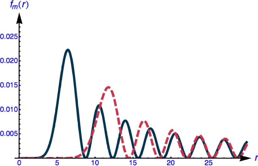
Figure 1: (Color online.) Plot of the radial probability density $f_{m}(r)=|\psi_{\varkappa m}(r,\varphi)|^{2}$ for $m=5$ (solid line) and $m=10$ (dashed line) at $\varkappa=1$. The central minimum of the wave function and the maximum at $r\sim m$ are clearly visible.

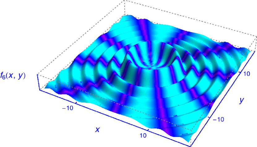
(a)

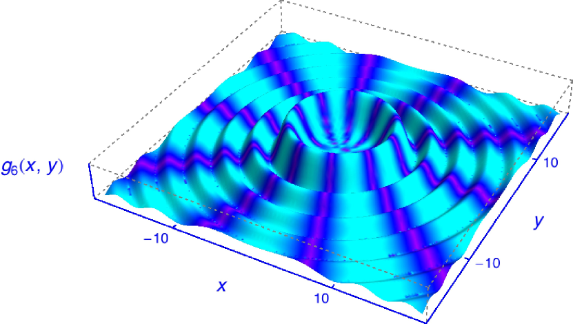
(b)

Figure 2: (Color online.) Illustration of the quantum vector potential ${{\cal A}}^{\mu}_{\varkappa mk_{z}\Lambda}$ of a twisted photon. The plot displays $f_{m}(x,y)=|{{\cal A}}^{\mu=1}_{\varkappa mk_{z}\Lambda}(0,x,y,0)|^{2}$ and $g_{m}(x,y)=|{{\cal A}}^{\mu=2}_{\varkappa mk_{z}\Lambda}(0,x,y,0)|^{2}$ as a function of $x$ and $y$. The parameters are $\varkappa=1$, $m=6$, $k_{z}=\sqrt{48}$, $\omega=\sqrt{\varkappa^{2}+k_{z}^{2}}=7$, and $\Lambda=1$. The complex phase of the vector potential (modulo $\pi$) is indicated by the variation of the color/grayscale of the wave function. Panels (a) and  (b) illustrate that the $x$ and $y$ components ($\mu=1$ versus $\mu=2$) of the twisted photon vector potentials are phase shifted with respect to each other.

2.2 Twisted photon

The wave function of a twisted photon (vector particle) can be constructed as a generalization of the scalar wave function. We start from the plane-wave photon state with a defined 4-momentum $k=(\omega,{\bm{k}})$ and helicity $\Lambda=\pm 1$,

$$A^{\mu}_{k\Lambda}(t,\bm{r})= \;\sqrt{4\pi}\,e^{\mu}_{k\Lambda}\,\frac{\mathrm{e}^{-\mathrm{i}(\omega\,t-{\bm{k}}{\bm{r}})}}{\sqrt{2\omega}}\,,$$ (12a)

$$e_{k\Lambda}\cdot k= \;0\,,\quad e^{*}_{k\Lambda}\cdot e_{k\Lambda^{\prime}}=-\delta_{\Lambda\Lambda^{\prime}}\,,$$ (12b)

where $e^{\mu}_{k\Lambda}$ is the polarization four-vector of the photon. The twisted photon vector potential

$${{\cal A}}^{\mu}_{\varkappa mk_{z}\Lambda}(r,\varphi_{r},z,t)=\int a_{\varkappa m}({\bm{k}}_{\perp})\,A^{\mu}_{k\Lambda}(t,\bm{r})\,\frac{\mathrm{d}^{2}k_{\perp}}{(2\pi)^{2}}$$ (13)

$$=(-\mathrm{i})^{m}\sqrt{2\pi\varkappa}\int\limits_{0}^{2\pi}\mathrm{d}\varphi_{k}\int\limits_{0}^{\infty}\mathrm{d}k_{\perp}\,\delta(k_{\perp}-\varkappa)\,\frac{e^{\mathrm{i}m\varphi_{k}}}{(2\pi)^{2}}\,A^{\mu}_{k\Lambda}(t,\bm{r})$$

is given as a two-fold integral over the perpendicular components ${\bm{k}}_{\perp}=(k_{x},k_{y},0)$ of the wave vector $\bm{k}=(k_{x},\,k_{y},\,k_{z})$. Using the well-known identity

$$\int_{0}^{\infty}\,J_{m}(\varkappa\,x)\,J_{m}(\varkappa^{\prime}\,x)\,x\,\mathrm{d}x=\frac{1}{\varkappa}\,\delta(\varkappa-\varkappa^{\prime})\,,$$ (14)

it is not difficult to prove that this function satisfies the normalization condition [compare with Eq. (2)]

$$\int\left({\cal A}^{*}_{\varkappa^{\prime}m^{\prime}k^{\prime}_{z}\Lambda^{\prime}}\right)_{\mu}(t,{\vec{r}})\,{\cal A}^{\mu}_{\varkappa mk_{z}\Lambda}(t,{\bm{r}})\,\mathrm{d}^{3}r$$

$$=-4\pi\delta_{\Lambda\Lambda^{\prime}}\,\frac{2\pi\delta(k_{z}-k^{\prime}_{z})}{2\omega}\delta_{mm^{\prime}}\delta(\varkappa-\varkappa^{\prime}).$$ (15)

We would like to stress that the orthogonal functions ${\cal A}^{\mu}_{\varkappa mk_{z}\Lambda}(t,{\bm{r}})$ for different values of $\varkappa,m,k_{z},\Lambda$ but fixed $z$ axis constitute a complete set of functions and can be used for the description of initial as well as final twisted photons.

The polarization vector $e_{k\Lambda}$ depends on the azimuth $\varphi_{k}$ as $\exp(\mathrm{i}\,\ell\varphi_{k})$ with $\ell=0,\,\pm 1$ depending on the helicity [see Eq. (4.1) below]. In view of the identity

$$\int\mathrm{e}^{\mathrm{i}\ell\varphi_{k}}\,a_{\varkappa m}({\bm{k}}_{\perp})\,\mathrm{e}^{\mathrm{i}{\bm{k}}_{\perp}{\bm{r}}}\,\frac{\mathrm{d}^{2}k_{\perp}}{(2\pi)^{2}}=\mathrm{i}^{\ell}\,\psi_{\varkappa,m+\ell}(r,\varphi_{r})\,,$$ (16)

the vector field ${\cal A}^{\mu}_{\varkappa mk_{z}\Lambda}(r,\varphi_{r},z,t)$ describes a photon state with defined $k_{z}$, absolute value of the transverse momentum $|{\bm{k}}_{\perp}|=\varkappa$, energy $\omega=\sqrt{\varkappa^{2}+k_{z}^{2}}$ and projection of the orbital angular momentum on the $z$ axis equal to $m-1,\,m,\,m+1$ [see also Eqs. (53)—(54) below]. Strictly speaking, this state is not a photon state with a defined value of $\check{L}_{z}$. However, for large $m$, the restriction to $(m-1,m,m+1)$ means that the twisted state is a state with a very restricted angular momentum projection distribution about the central value equal to $m$. The representation (16) is very convenient as it allows us to considerably simplify the analytic calculations. We call such a state a twisted $m$ photon (see Fig. 2) and denote it as $|\varkappa,m,k_{z},\Lambda\rangle$.

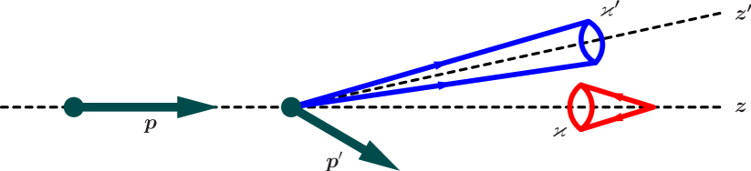
Figure 3: (Color online.) Schematic view of the scattering geometry. The incoming twisted photon with transverse momentum spread $\varkappa$ is scattered by a counterpropagating electron with momentum $p$, into a state propagating along an arbitrary $z^{\prime}$ axis with transverse momentum spread $\varkappa^{\prime}$, with the electron assuming momentum $p^{\prime}$. For the specific case of strict backward Compton scattering, the $z$ and $z^{\prime}$ axes and the vectors ${\bm{p}}$ and ${\bm{p}}^{\prime}$ are all collinear.

The usual $S$ matrix element for plane-wave (PW) Compton scattering involves an electron being scattered from the state $|p,\lambda\rangle$ with 4-momentum $p$ and helicity $\lambda=\pm\tfrac{1}{2}$ to a state $|p^{\prime},\lambda^{\prime}\rangle$ and a photon being scattered from the state $|k,\Lambda\rangle$ to the state $|k^{\prime},\Lambda^{\prime}\rangle$,

$$S^{\rm(PW)}_{fi}\equiv\langle k^{\prime},\Lambda^{\prime},p^{\prime},\lambda^{\prime}|S|k,\Lambda,p,\lambda\rangle\,.$$ (17)

For head-on collisions, the vectors ${\bm{p}}=(0,0,p_{z})$ and ${\bm{k}}=(0,0,-\omega)$ are anti-parallel.

Let us consider the Compton effect for the case when an initial plane-wave electron in the state $|p,\lambda\rangle$ performs a head-on collision with an initial twisted $m$ photon $|\varkappa,m,k_{z},\Lambda\rangle$ propagating along the $(-z)$ axis. In the final state, there is a plane-wave electron $|p^{\prime},\lambda^{\prime}\rangle$ and a final twisted $m^{\prime}$ photon $|\varkappa^{\prime},m^{\prime},k^{\prime}_{z},\Lambda^{\prime}\rangle$ propagating along the $z^{\prime}$ axis (a schematic view of the initial and final states is given in Fig. 3). As noted above, we can choose the $z^{\prime}$ axis along an arbitrary direction, but below we restrict the discussion to the particular scattering geometry where the axes $z^{\prime}$ and $z$ are naturally defined as being collinear, namely, the strict backscattering geometry. (Moreover, even in a general case it is convenient to choose the $z^{\prime}$ axis along the $z$ axis, leading to a potential simplification of the calculation.) In view of Eq. (13), the $S$ matrix element for such a scattering,

$$S^{\rm(TW)}_{fi}\equiv\langle\varkappa^{\prime},m^{\prime},k^{\prime}_{z},\lambda^{\prime};p^{\prime},\lambda^{\prime}|S|\varkappa,m,k_{z},\Lambda;p,\lambda\rangle,$$ (18)

needs to be integrated as follows,

$$S^{\rm(TW)}_{fi}\equiv \;\int\frac{\mathrm{d}^{2}k_{\perp}}{(2\pi)^{2}}\,\frac{\mathrm{d}^{2}k^{\prime}_{\perp}}{(2\pi)^{2}}\,a^{*}_{\varkappa^{\prime}m^{\prime}}({\bm{k}}^{\prime}_{\perp})\;$$ (19)

$$\times\langle k^{\prime},\Lambda^{\prime},p^{\prime},\lambda^{\prime}|S|k,\Lambda,p,\lambda\rangle\,a_{\varkappa m}({\bm{k}}_{\perp})$$

$$= \;\int\frac{\mathrm{d}^{2}k_{\perp}}{(2\pi)^{2}}\,\frac{\mathrm{d}^{2}k^{\prime}_{\perp}}{(2\pi)^{2}}\,a^{*}_{\varkappa^{\prime}m^{\prime}}({\bm{k}}^{\prime}_{\perp})\;S^{\rm(PWC)}_{fi}\;a_{\varkappa m}({\bm{k}}_{\perp})\,,$$

where by PWC we denote the scattering matrix elements for the plane-wave component of the twisted photons, with 4-vector components $k=(\omega,\bm{k}_{\perp},k_{z})$ and $k^{\prime}=(\omega^{\prime},\bm{k}^{\prime}_{\perp},k_{z}^{\prime})$.

Based on Eq. (11), we conclude that the integration in Eq. (19) is determined by the dependence of the matrix element $S^{\rm(PWC)}_{fi}$ on the azimuthal angles $\varphi_{k}$ and $\varphi^{\prime}_{k}$ of the vectors ${\bm{k}}$ and ${\bm{k}}^{\prime}$. A numerical integration of Eq. (19) then leads to predictions for arbitrary scattering angle of the final electron. In this paper we consider in detail the important case of strict backward Compton scattering when the scattering angle of the final electron equals zero and the vector ${\bm{p}}^{\prime}$ is directed along the $z$ axis. Such a choice is determined mainly by two reasons. First of all, for usual Compton scattering on ultra-relativistic unpolarized electrons, precisely the backward scattering has the largest probability (see Fig. 4 below). Second, the matrix element $S^{\rm(PWC)}_{fi}$ does not depend on the azimuthal angles $\varphi_{k}$ and $\varphi^{\prime}_{k}$, and therefore, this case allows for a simple and transparent treatment with analytical calculations for usual as well as for twisted photons.

3 Compton scattering of plane-wave photons

3.1 General formulas

In principle, Compton backscattering is an established method for the creation of high-energy photons and used successfully in various application areas from the study of photo-nuclear reactions NeTuSh2004 to colliding photon beams of high energy BaEtAl2004 ; Se2006appb . Let us consider the collision of an ultra-relativistic electron with four momentum

$$p=(E,0,0,vE),\;\;v=\frac{|{\bm{p}}|}{E},\;\;\gamma=\frac{E}{m_{e}}\,,$$ (20)

whose spatial momentum component points strictly upward, and a photon of energy $\omega$ and three-momentum

$${\bm{k}}=\omega\;(\sin{\alpha_{0}}\,\cos{\varphi_{k}},\;\sin{\alpha_{0}}\,\sin{\varphi_{k}},\;-\cos{\alpha_{0}})\,.$$ (21)

Here, $\theta=\pi-\alpha_{0}$ and $\varphi_{k}$ are the polar and azimuthal angles of the initial photon. For a downward pointing photon (head-on collision), we have $\alpha_{0}=0$. After the scattering, the four-momentum of the electron is $p^{\prime}$, and the scattered photon has energy $\omega^{\prime}$ and three-momentum

$${\bm{k}}^{\prime}=\omega^{\prime}(\sin{\theta^{\prime}}\cos{\varphi^{\prime}_{k}},\;\sin{\theta^{\prime}}\sin{\varphi^{\prime}_{k}},\;\cos{\theta^{\prime}})\,,$$ (22)

where $\theta^{\prime}$ and $\varphi^{\prime}_{k}$ are the polar and azimuthal angles of the final photon. Let $\beta$ be the angle between the vectors ${\bm{k}}^{\prime}$ and $(-{\bm{k}})$. For head-on backscattering, we have $\beta=0$. In general,

$${\bm{k}}{\bm{k}}^{\prime}=-\omega\;\omega^{\prime}\;\cos{\beta}\,,$$ (23)

and

$$\cos{\beta}=\cos{\alpha_{0}}\,\cos{\theta^{\prime}}-\sin{\alpha_{0}}\,\sin{\theta^{\prime}}\,\cos{(\varphi_{k}-\varphi^{\prime}_{k}})\,.$$ (24)

From the on-mass-shell condition of the scattered electron, we have $p^{\prime 2}=(p+k-k^{\prime})^{2}=m_{e}^{2}$, and therefore $k^{\prime}\cdot(p+k)=k\cdot p$ or

$$\omega^{\prime}=\frac{m_{e}^{2}\,x}{2E(1-v\cos{\theta^{\prime}})+2\omega(1+\cos{\beta})}\,,$$ (25)

where

$$x=\frac{2\,k\cdot p}{m_{e}^{2}}=\frac{2\omega E(1+v\cos{\alpha_{0}})}{m_{e}^{2}}\,.$$ (26)

The $S$ matrix element for plane waves (either plane direct incoming and outgoing plane waves or plane-wave components of a twisted photon) is

$$\langle k^{\prime},\Lambda^{\prime},p^{\prime},\lambda^{\prime}|S|k,\Lambda,p,\lambda\rangle$$

$$\qquad=\mathrm{i}\,(2\pi)^{4}\,\delta(p+k-p^{\prime}-k^{\prime})\;\frac{M_{fi}}{4\sqrt{E\,E^{\prime}\,\omega\,\omega^{\prime}}}\,,$$ (27)

where the scattering amplitude $M_{fi}$ in the Feynman gauge is equal to

$$M_{fi} = 4\pi\alpha\left(\frac{A}{s-m_{e}^{2}}+\frac{B}{u-m_{e}^{2}}\right)\,,$$ (28a)

$$A = \bar{u}_{p^{\prime}\lambda^{\prime}}\,\hat{e}^{*}_{k^{\prime}\Lambda^{\prime}}\,\left(\hat{p}+\hat{k}+m_{e}\right)\hat{e}_{k\Lambda}\,u_{p\lambda}\,,$$ (28b)

$$B = \bar{u}_{p^{\prime}\lambda^{\prime}}\,\hat{e}_{k\Lambda}\left(\hat{p}^{\prime}-\hat{k}+m_{e}\right)\hat{e}^{*}_{k^{\prime}\Lambda^{\prime}}\,u_{p\lambda}\,,$$ (28c)

$$s-m_{e}^{2} = 2k\cdot p=m_{e}^{2}x\,,\;\;u-m_{e}^{2}=-2k^{\prime}\cdot p\,.$$ (28d)

The bispinors $u_{p\lambda}$ and $u_{p^{\prime}\lambda^{\prime}}$ describe the initial and final electrons with helicities $\lambda$ and $\lambda^{\prime}$, and $e_{k\Lambda}$ and $e_{k^{\prime}\Lambda^{\prime}}$ are the polarization vectors of the initial and final photons with helicities $\Lambda$ and $\Lambda^{\prime}$. We denote the Feynman dagger as $\hat{p}=\gamma^{\mu}p_{\mu}$.

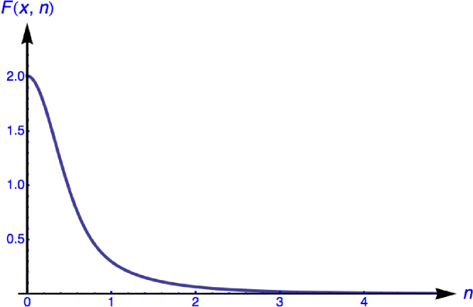
Figure 4: The angular distribution $\mathrm{d}\sigma/\mathrm{d}\Omega^{\prime}=2\alpha^{2}\,\gamma^{2}\,m_{e}^{-2}\,F(x,n)$ of the final photons in the Compton scattering in dependence on $n=\gamma\,\theta^{\prime}$. The value $x=0.092$ corresponds to the VEPP-4M collider.

For Compton scattering off incoming ultra-relativistic electrons ($\gamma\gg 1$), the differential cross section has a maximum in the backscattering region, where the polar angle of the scattered photon is small, $\theta^{\prime}\lesssim 1/\gamma$, and the photon propagates almost along the direction of momentum of the initial electron. Indeed, for unpolarized electrons, the differential Compton cross section reads BeLiPi1982vol4

$$\frac{\mathrm{d}\sigma}{\mathrm{d}\Omega^{\prime}} = \frac{2\alpha^{2}\gamma^{2}}{m_{e}^{2}}\,F(x,n),$$ (29)

$$F(x,n) = \left(\frac{1}{1+x+n^{2}}\right)^{2}\left[\frac{1+x+n^{2}}{1+n^{2}}\right.$$

$$\left.+\frac{1+n^{2}}{1+x+n^{2}}-4\,\frac{n^{2}}{(1+n^{2})^{2}}\right]\,,$$

where $n=\gamma\,\theta^{\prime}$, $\mathrm{d}\Omega^{\prime}=\sin{\theta^{\prime}}\mathrm{d}{\theta^{\prime}}\mathrm{d}\varphi^{\prime}_{k}$, and

$$\frac{\omega^{\prime}}{\omega}=\frac{4\gamma^{2}}{1+x+n^{2}}\,.$$ (30)

In Fig. 4, we show the angular distribution of the final photons which is concentrated to the region $n\lesssim 1$. The value of $x$ used, namely $x=0.092$, corresponds to the collider parameter $x$ as defined in Eq. (26), evaluated for the VEPP-4M collider (Novosibirsk) with $E=5\,{\rm GeV}$ and $\omega=1.2$ eV. The maximum energy of the final photon is $\omega^{\prime}=420\,{\rm MeV}$ for $\theta^{\prime}=0$. For $n\lesssim 1$, the energy $\omega^{\prime}$ of the final photon is independent of the azimuth angle $\varphi_{k}$ or $\varphi^{\prime}_{k}$,

$$\omega^{\prime}=\frac{x}{1+x+(\gamma\theta^{\prime})^{2}}\;E\,.$$ (31)

To make calculations in the main region more transparent, it is useful to decompose the scattering amplitude (28a) into dominant and negligible items. To do this, in the $A$ term defined in Eq. (28b), we transpose $\hat{e}_{k\Lambda}$ and $\hat{p}+\hat{k}+m_{e}$ using the Dirac equation and obtain

$$\left(\hat{p}+\hat{k}+m_{e}\right)\hat{e}_{k\Lambda}\,u_{p\lambda}=\;\hat{e}_{k\Lambda}(-\hat{p}-\hat{k}+m_{e})\,u_{p\lambda}$$

$$\quad+2(e_{k\Lambda}\cdot p)\,u_{p\lambda}=\;-\hat{e}_{k\Lambda}\hat{k}\,u_{p\lambda}+2(e_{k\Lambda}\cdot p)\,u_{p\lambda}\,.$$ (32)

Thus, $A=A_{1}+A_{2}$ with

$$A_{1}= \;-\bar{u}_{p^{\prime}\lambda^{\prime}}\;\hat{e}_{k^{\prime}\Lambda^{\prime}}^{*}\;\hat{e}_{k\Lambda}\;\hat{k}\,u_{p\lambda}\,,$$ (33a)

$$A_{2}= \;2(e_{k\Lambda}\cdot p)\;\bar{u}_{p^{\prime}\lambda^{\prime}}\;\hat{e}_{k^{\prime}\Lambda^{\prime}}^{*}\;u_{p\lambda}\,.$$ (33b)

In full analogy, $$B=B_{1}+B_{2}$$ with

$$B_{1}= \;\bar{u}_{p^{\prime}\lambda^{\prime}}\;\hat{k}\;\hat{e}_{k\Lambda}\;\hat{e}_{k^{\prime}\Lambda^{\prime}}^{*}\;u_{p\lambda}\,,\;\;$$ (33c)

$$B_{2}= \;2(e_{k\Lambda}\cdot p^{\prime})\;\bar{u}_{p^{\prime}\lambda^{\prime}}\;\hat{e}_{k^{\prime}\Lambda^{\prime}}^{*}\;u_{p\lambda}\,.$$ (33d)

The scattering amplitude $M_{fi}$ as defined in Eq. (28a) can thus be written as

$$M_{fi}= \;M_{1}+M_{2}\,,$$ (34a)

$$M_{1}= \;4\pi\alpha\left(\frac{A_{1}}{s-m_{e}^{2}}+\frac{B_{1}}{u-m_{e}^{2}}\right)\,,$$ (34b)

$$M_{2}= \;4\pi\alpha\left(\frac{A_{2}}{s-m_{e}^{2}}+\frac{B_{2}}{u-m_{e}^{2}}\right)\,.$$ (34c)

The term $M_{1}$ will be shown to play the dominant role in our calculation. For further analysis we also introduce three 4-vectors,

$$\eta^{(\pm)}=\frac{\mp 1}{\sqrt{2}}\,(0,\,1,\pm\mathrm{i},\,0)\,,\;\;\eta^{(z)}=(0,\,0,\,0,\,1)\,.$$ (35)

3.2 Strict backward Compton scattering

For a head-on collision of a plane-wave photon and a counter-propagating electron, the electron after scattering moves in the same direction as before the collision, but with a smaller energy $E^{\prime}$,

$$p^{\prime}=(E^{\prime},0,0,v^{\prime}E^{\prime}),\;\;v^{\prime}=\frac{|{\bm{p}}^{\prime}|}{E^{\prime}}\,.$$ (36)

For plane waves, strict backward scattering has the largest probability (see Fig. 4), and this case allows for a simplified treatment. Indeed, for strict backward geometry, we have $k^{\prime}_{\perp}=k_{\perp}=0$, and the photon polarization vectors can be chosen in the form

$$e_{k^{\prime},\pm 1}=e_{k,\mp 1}=\eta^{(\pm)}\,.$$ (37)

For the considered head-on collision, we have

$$e_{k\Lambda}\cdot p= \;0\,,\qquad e_{k\Lambda}\cdot p^{\prime}=0\,,$$ (38a)

$$A_{2}= \;0\,,\qquad B_{2}=0\,,$$ (38b)

i.e. the term $M_{2}^{\rm(PW)}$ vanishes for plane-wave strict backward scattering.

In order to calculate $A_{1}$ as given by Eq. (33a), it is useful to represent the expression $\hat{e}_{k^{\prime}\Lambda^{\prime}}^{*}\,\hat{e}_{k\Lambda}$ as

$$2\,\hat{e}_{k^{\prime}\Lambda^{\prime}}^{*}\,\hat{e}_{k\Lambda}= \;\Lambda\Lambda^{\prime}-1+\left(\Lambda^{\prime}-\Lambda\right)\Sigma_{z}$$

$$= -2\,\left(1+\Lambda\Sigma_{z}\right)\,\delta_{\Lambda,-\Lambda^{\prime}}\,,$$ (39)

where $\frac{1}{2}{\bm{\Sigma}}$ is a $4\times 4$ matrix vector measuring the electron spin. Substituting this expression into $A_{1}$, we find

$$A^{\rm(PW)}_{1}=8\omega\sqrt{EE^{\prime}}\,\delta_{\lambda\lambda^{\prime}}\,\delta_{\Lambda,-\Lambda^{\prime}}\,\delta_{2\lambda,\Lambda}$$ (40a)

and, analogously,

$$B^{\rm(PW)}_{1}=-8\omega\sqrt{EE^{\prime}}\,\delta_{\lambda\lambda^{\prime}}\,\delta_{\Lambda,-\Lambda^{\prime}}\,\delta_{2\lambda,-\Lambda}\,.$$ (40b)

Further important kinematic relations are

$$s-m_{e}^{2}=m_{e}^{2}\;x\,,\qquad u-m_{e}^{2}=-\frac{m_{e}^{2}\;x}{x+1}\,.$$ (41)

As a result, the scattering amplitude for plane-wave strict backward scattering is

$$M^{\rm(PW)}_{fi}= \;M_{1}^{\rm(PW)}=\frac{8\pi\alpha}{\sqrt{x+1}}\left[\delta_{2\lambda,\Lambda}\right.$$

$$\left.+(x+1)\delta_{2\lambda,-\Lambda}\right]\,\delta_{\lambda\lambda^{\prime}}\,\delta_{\Lambda,-\Lambda^{\prime}}\,,$$ (42)

with $x=4\omega E/m_{e}^{2}$. We emphasize that in head-on backscattering, the electron does not change its helicity during scattering ($\lambda^{\prime}=\lambda$) while the photon does change its helicity, $\Lambda^{\prime}=-\Lambda$. All these results are in full agreement with known properties of ordinary Compton scattering BeLiPi1982vol4 ; GiKoPoSeTe1984 ; KoPoSe1998 .

4 Compton backscattering of twisted photons

4.1 Kinematics

In the case of a twisted photon, the final $m^{\prime}$ photon state $|\varkappa^{\prime},m^{\prime},k_{z}^{\prime},\Lambda^{\prime}\rangle$ is a superposition of plane waves with high energy, consistent with the general principle of Compton backscattering. The transverse momentum is conserved,

$${\bm{k}}^{\prime}_{\perp}={\bm{k}}_{\perp}\,,$$ (43)

as can be seen from the conservation law $k+p=k^{\prime}+p^{\prime}$, which follows from the fact that the transverse components of the vectors $p$ and $p^{\prime}$ are equal to zero. The scattering angle is very small,

$$\theta^{\prime}=\frac{k^{\prime}_{\perp}}{\omega^{\prime}}\lesssim\frac{\omega}{\omega^{\prime}}=\frac{1+x+n^{2}}{4\gamma^{2}}\approx\frac{1+x}{4\gamma^{2}}\,.$$ (44)

From Eq. (43), we have $\varphi_{k}^{\prime}=\varphi_{k}$, and the energy of the scattered photon is

$$\omega^{\prime}=\frac{x}{1+x}\,E\,,$$ (45)

as evident from Eq. (31) in the limit $\theta^{\prime}\to 0$.

In view of the structure of the plane-wave scattering element recorded in Eq. (3.1), the convoluted matrix element for backward scattering of twisted photons given in Eq. (19) takes the form

$$S^{\rm(TW)}_{fi}=\mathrm{i}\,2\pi\,\mathrm{i}^{m^{\prime}-m}\delta(\varkappa-\varkappa^{\prime})\frac{1}{4\sqrt{EE^{\prime}\omega\omega^{\prime}}}$$ (46)

$$\times\delta(E+\omega-E^{\prime}-\omega^{\prime})\,\delta(p_{z}+k_{z}-p_{z}^{\prime}-k_{z}^{\prime})$$

$$\times\int\limits_{0}^{2\pi}{\mathrm{e}^{\mathrm{i}(m-m^{\prime})\varphi_{k}}}\left(M_{1}^{\rm(PWC)}+M_{2}^{\rm(PWC)}\right)\mathrm{d}\varphi_{k}\,,$$

where we have used the decomposition (34), and $M_{1}^{\rm(PWC)}$ and $M_{2}^{\rm(PWC)}$ are the plane-wave components of the twisted photon scattering matrix element. Note that $M_{1}^{\rm(PWC)}$ and $M_{2}^{\rm(PWC)}$ are not equal to their plane-wave counterparts $M_{1}^{\rm(PW)}$ and $M_{2}^{\rm(PW)}$ because of the nonvanishing conical momentum spread of the twisted photon.

The admissible values of $m^{\prime}$ are determined by the dependence of $A$ and $B$ on $\varphi_{k}$. In order to carry out the integration over $\varphi_{k}$, we have to analyze the dependence of the polarization vectors $e_{k\Lambda}$ and $e_{k^{\prime}\Lambda^{\prime}}$ on the azimuth angle. To this end, we choose the polarization vector of the final photon in the scattering amplitude $M_{fi}$ in the form

$$e_{k^{\prime}\Lambda^{\prime}}=-\frac{\Lambda^{\prime}}{\sqrt{2}}\,\left(e^{(x^{\prime})}+\mathrm{i}\Lambda^{\prime}\,e^{(y^{\prime})}\right)\,,$$ (47)

where the unit vector $e^{(x^{\prime})}=(0,\,{\bm{e}}^{(x^{\prime})})$ is in the scattering plane, defined by the vectors $\bm{p}\parallel\bm{p}^{\prime}$ and $\bm{k}^{\prime}$, while the unit vector $e^{(y^{\prime})}$ is orthogonal to it,

$${\bm{e}}^{(x^{\prime})}\,\parallel\;({\bm{p}}\times{\bm{k}}^{\prime})\times{\bm{k}}^{\prime}\,,\qquad{\bm{e}}^{(y^{\prime})}\,\parallel\;({\bm{p}}\times{\bm{k}}^{\prime})\,.$$ (48)

As a result, we have in four-vector component notation

$$e_{k^{\prime}\Lambda^{\prime}}=-\frac{\Lambda^{\prime}}{\sqrt{2}}\,\left(\begin{array}[]{c}0\\ \cos{\theta^{\prime}}\cos{\varphi_{k}}-\mathrm{i}\Lambda^{\prime}\sin{\varphi_{k}}\\ \cos{\theta^{\prime}}\sin{\varphi_{k}}+\mathrm{i}\Lambda^{\prime}\cos{\varphi_{k}}\\ -\sin{\theta^{\prime}}\end{array}\right)\,.$$ (49)

Omitting small terms of the order of $\theta^{\prime}$, this vector becomes

$$e_{k^{\prime}\Lambda^{\prime}}=-\frac{\Lambda^{\prime}}{\sqrt{2}}\,(0,\,1,\,\mathrm{i}\Lambda^{\prime},\,0)\,\mathrm{e}^{-\mathrm{i}\Lambda^{\prime}\varphi_{k}}=\eta^{(\Lambda^{\prime})}\,\mathrm{e}^{-\mathrm{i}\Lambda^{\prime}\varphi_{k}}\,.$$ (50)

The polarization vector $e_{k\Lambda}$ of a conical component of the initial twisted photon (as a function of $\varphi_{k}$) is obtained by setting $\theta^{\prime}=\pi-\alpha_{0}$ in $e_{k^{\prime}\Lambda^{\prime}}$ and reads

$$e_{k\Lambda}=\frac{\Lambda}{\sqrt{2}}\,\left(\begin{array}[]{c}0\\ \cos{\alpha_{0}}\cos{\varphi_{k}}+\mathrm{i}\Lambda\sin{\varphi_{k}}\\ \cos{\alpha_{0}}\sin{\varphi_{k}}-\mathrm{i}\Lambda\cos{\varphi_{k}}\\ \sin{\alpha_{0}}\end{array}\right)\,.$$ (51)

Using the 4-vectors defined in Eq. (35), we may write it in the form

$$e_{k\Lambda}= \;\eta^{(-\Lambda)}\,\mathrm{e}^{\mathrm{i}\Lambda\varphi_{k}}\,\cos^{2}\left(\frac{\alpha_{0}}{2}\right)+\eta^{(\Lambda)}\,\mathrm{e}^{-\mathrm{i}\Lambda\varphi_{k}}\,\sin^{2}\left(\frac{\alpha_{0}}{2}\right)$$

$$\;+\frac{\Lambda}{\sqrt{2}}\,\eta^{(z)}\,\sin{\alpha_{0}}\,.$$ (52)

With the help of Eq. (16), we can also write the Fourier transform of the product $e_{k\Lambda}\,a_{\varkappa m}({\bm{k}}_{\perp})$, which is still a 4-vector, as

$$I_{\varkappa m\Lambda}= \;\int e_{k\Lambda}\,a_{\varkappa m}({\bm{k}}_{\perp})\,\mathrm{e}^{\mathrm{i}\,{\bm{k}}_{\perp}{\bm{r}}}\frac{\mathrm{d}^{2}k_{\perp}}{(2\pi)^{2}}$$ (53)

$$= \;\mathrm{i}^{\Lambda}\;\eta^{(-\Lambda)}\;\psi_{\varkappa,m+\Lambda}(r,\varphi_{r})\,\cos^{2}\left(\frac{\alpha_{0}}{2}\right)$$

$$- \;\mathrm{i}^{\Lambda}\;\eta^{(\Lambda)}\;\psi_{\varkappa,m-\Lambda}(r,\varphi_{r})\,\sin^{2}\left(\frac{\alpha_{0}}{2}\right)$$

$$+ \;\frac{\Lambda}{\sqrt{2}}\,\eta^{(z)}\,\psi_{\varkappa m}(r,\varphi_{r})\,\sin{\alpha_{0}}\,,$$

recalling that the function $\psi_{\varkappa m}(r,\varphi_{r})$ is given in Eq. (2.1). With this formula for $I_{\varkappa m\Lambda}$, we can write the twisted photon vector potential (13) as

$${\cal A}^{\mu}_{\varkappa mk_{z}\Lambda}(r,\varphi_{r},z,t)=\;\sqrt{4\pi}\;\frac{\mathrm{e}^{-\mathrm{i}(\omega t-k_{z}z)}}{\sqrt{2\omega}}\;I^{\mu}_{\varkappa m\Lambda}\,.$$ (54)

This 4-vector potential corresponds to the initial twisted photon state $|\varkappa,m,k_{z},\Lambda\rangle$, which describes a superposition of states with projections of the orbital angular momentum onto the $z$ axis equal to $m$ and $m\pm\Lambda$. If the angle $\alpha_{0}$ becomes small, we have

$$|\varkappa,m,k_{z},\Lambda\rangle\propto\eta^{(-\Lambda)}\;\psi_{\varkappa,m+\Lambda}(r,\varphi_{r})\,,$$ (55)

and the projection $m+\Lambda$ becomes dominant. For the final twisted photon with its small angle $\theta^{\prime}$, we have

$$|\varkappa^{\prime},m^{\prime},k_{z}^{\prime},\Lambda^{\prime}\rangle\propto\eta^{(\Lambda^{\prime})}\;\psi_{\varkappa^{\prime},m^{\prime}-\Lambda^{\prime}}(r,\varphi_{r}),$$ (56)

and, therefore, the projection $m^{\prime}-\Lambda^{\prime}$ is dominant.

4.2 Main $\maybebm{S}$ matrix contribution for twisted photons

For backward scattering of twisted photons, the incoming and outgoing polarization vectors are given by Eqs. (51) and (50), respectively. Investigating the contribution from $A_{1}$ given by (33a), we write $\hat{e}_{k^{\prime}\Lambda^{\prime}}^{*}\,\hat{e}_{k\Lambda}$ in the form

$$2\hat{e}_{k^{\prime}\Lambda^{\prime}}^{*}\;\hat{e}_{k\Lambda} =-(1-\Lambda\Lambda^{\prime}\cos{\alpha_{0}})\,(1-\Lambda^{\prime}\Sigma_{z})$$

$$\quad+\Lambda\,\left(\Sigma_{x}-\mathrm{i}\,\Lambda^{\prime}\,\Sigma_{y}\right)\,\mathrm{e}^{\mathrm{i}\Lambda^{\prime}\varphi_{k}}\,.$$ (57)

Substituting this expression in $A_{1}$, we find

$$A_{1}^{\rm(PWC)}= \;2\omega\,\sqrt{EE^{\prime}}\,\left[(1-\Lambda\,\Lambda^{\prime}\cos{\alpha_{0}})\,(1+\cos{\alpha_{0}})\right.$$

$$\;\left.+2\lambda\,\Lambda\,\sin^{2}{\alpha_{0}}\right]\,\delta_{\lambda\lambda^{\prime}}\,\delta_{2\lambda,-\Lambda^{\prime}}\,.$$ (58a)

Analogously,

$$B_{1}^{\rm(PWC)}= -2\omega\,\sqrt{EE^{\prime}}\,\left[(1-\Lambda\,\Lambda^{\prime}\cos{\alpha_{0}})\,(1+\cos{\alpha_{0}})\right.$$

$$\;\left.-2\lambda\,\Lambda\,\sin^{2}{\alpha_{0}}\right]\,\delta_{\lambda\lambda^{\prime}}\,\delta_{2\lambda,\Lambda^{\prime}}\,.$$ (58b)

For $\alpha_{0}=0$, the expressions $A_{1}^{\rm(PWC)}$ and $B_{1}^{\rm(PWC)}$ for twisted backscattering become proportional to the Kronecker delta of the helicities $\delta_{\Lambda,-\Lambda^{\prime}}$, and Eqs. (58) and (58) coincide with Eqs. (40a) and (40b), respectively. However, for a twisted photon, $\alpha_{0}=\arctan[\varkappa/(-k_{z})]\neq 0$ and the value $\Lambda^{\prime}=\Lambda$ is possible. Nevertheless, the corresponding probability for $\Lambda^{\prime}=\Lambda$ is small for small values of the colliding angle $\alpha_{0}$ because in this case, $A_{1}^{\rm(PWC)}\propto\sin^{2}(\alpha_{0}/2)$ and $B_{1}^{\rm(PWC)}\propto\sin^{2}(\alpha_{0}/2)$.

None of the quantities $A_{1}^{\rm(PWC)}$, $B_{1}^{\rm(PWC)}$ nor $M_{1}^{\rm(PWC)}$ depend on $\varphi_{k}$. This could be expected because in the considered case, the colliding plane (determined by the vectors ${\bm{p}}$ and ${\bm{k}}_{\perp}$) coincides with the scattering plane (determined by the vectors ${\bm{p}}$ and ${\bm{k}}^{\prime}_{\perp}={\bm{k}}_{\perp}$). The integral over $\varphi_{k}$ in Eq. (46) is trivial, and we thus have $m^{\prime}=m$ in the term $M_{1}^{\rm(PWC)}$. Finally,

$$\int\limits_{0}^{2\pi}{\mathrm{e}^{\mathrm{i}(m-m^{\prime})\varphi_{k}}}M_{1}^{\rm(PWC)}\mathrm{d}\varphi_{k}=2\pi\,\delta_{mm^{\prime}}\,M_{1}^{\rm(PWC)}\,,$$ (59)

with

$$M_{1}^{\rm(PWC)}=4\pi\alpha\;\left(\frac{A_{1}^{\rm(PWC)}}{s-m_{e}^{2}}+\frac{B_{1}^{\rm(PWC)}}{u-m_{e}^{2}}\right)\,.$$ (60)

The quantities $A_{1}^{\rm(PWC)}$ and $B_{1}^{\rm(PWC)}$ are given in Eqs. (58) and (58).

Collecting all prefactors, we can establish the following structure for the $S$ matrix element (19) for strict backward Compton scattering of twisted photons,

$$S^{\rm(TW)}_{fi}= \;\langle\varkappa^{\prime},m^{\prime},k^{\prime}_{z},\Lambda^{\prime};p^{\prime},\lambda^{\prime}|S|\varkappa,m,k_{z},\Lambda;p,\lambda\rangle$$

$$= \;\mathrm{i}\,(2\pi)^{2}\,\delta_{mm^{\prime}}\,\delta(\varkappa-\varkappa^{\prime})\,\delta(E+\omega-E^{\prime}-\omega^{\prime})$$

$$\;\times\;\delta(p_{z}+k_{z}-p_{z}^{\prime}-k_{z}^{\prime})\frac{M_{1}^{\rm(PWC)}}{4\sqrt{EE^{\prime}\omega\omega^{\prime}}}\,.$$ (61)

4.3 Neglected contribution $\maybebm{M_{2}^{\rm(PWC)}}$

Let us consider the terms $A_{2}^{\rm(PWC)}$ and $B_{2}^{\rm(PWC)}$ which enter the expression (34) for $M_{2}^{\rm(PWC)}$. These items do not vanish, as for plane-wave strict backscattering, but there are large cancellations among them. We write $M_{2}^{\rm(PWC)}$ as follows,

$$M_{2}^{\rm(PWC)}= \;4\pi\alpha\;\bar{u}_{p^{\prime}\lambda^{\prime}}\,\hat{e}_{k^{\prime}\Lambda^{\prime}}^{*}\,u_{p\lambda}\,\left(\frac{e_{k\Lambda}\cdot p}{k\cdot p}-\frac{e_{k\Lambda}\cdot p^{\prime}}{k\cdot p^{\prime}}\right)$$

$$= \;-4\pi\alpha\;\bar{u}_{p^{\prime}\lambda^{\prime}}\,\hat{e}_{k^{\prime}\Lambda^{\prime}}^{*}\,u_{p\lambda}\,\frac{(e_{k\Lambda})_{z}}{\omega}\,\epsilon\,,$$ (62)

where the quantity

$$\epsilon=\omega\,\left(\frac{p_{z}}{k\cdot p}-\frac{p^{\prime}_{z}}{k\cdot p^{\prime}}\right)$$ (63)

is very small due to mutual cancellations,

$$\epsilon= \;\frac{v}{1+v\cos{\alpha_{0}}}-\frac{v^{\prime}}{1+v^{\prime}\cos{\alpha_{0}}}$$

$$= \;\frac{m_{e}^{2}}{2E^{2}}\,\frac{x(x+2)}{(1+\cos{\alpha_{0}})^{2}}\ll 1\,.$$ (64)

Finally,

$$\bar{u}_{p^{\prime}\lambda^{\prime}}\;e_{k^{\prime}\Lambda^{\prime}}^{*}\;u_{p\lambda}=\sqrt{2}\,\mathrm{e}^{\mathrm{i}\,\Lambda^{\prime}\varphi_{k}}\;\frac{m_{e}\,\omega^{\prime}}{\sqrt{EE^{\prime}}}\,\delta_{\lambda,-\lambda^{\prime}}\,\delta_{2\lambda,-\Lambda^{\prime}}\,.$$ (65)

The main contribution in this result is given by the transverse component of the vector ${e}_{k^{\prime}\Lambda^{\prime}}$, while the longitudinal component $\left(e_{k^{\prime}\Lambda^{\prime}}\right)_{z}$ gives only a small contribution,

$$|\bar{u}_{p^{\prime}\lambda^{\prime}}\;\left(\hat{e}_{k^{\prime}\Lambda^{\prime}}\right)_{z}^{*}\;u_{p\lambda}|\lesssim\frac{\omega}{\omega^{\prime}}\,\sqrt{EE^{\prime}}\,,$$ (66)

since $|\left(e_{k^{\prime}\Lambda^{\prime}}\right)_{z}|\lesssim\theta^{\prime}$. In view of Eq. (4.3), we have $|M_{2}^{\rm(PWC)}|\ll|M_{1}^{\rm(PWC)}|$ due to the mutual cancellations of large contributions from $s$ and $u$ channels. We can thus neglect $M_{2}^{\rm(PWC)}$ in strict backward scattering.

4.4 Averaged cross section for twisted photons

We base our considerations in this section on the approach described in Ref. BeLiPi1982vol4 , taking into account the necessary modifications for twisted photons. Compton scattering needs to be considered in a large but finite space-time volume $T\,V$, with time duration $T$ and spatial volume $V$. The normalization of plane-wave particles with $V=L_{x}L_{y}L_{z}$ as well as twisted photons with $V=\pi R^{2}L_{z}$ is discussed in detail in the Appendices A and B.

The $S$ matrix element for the Compton scattering of plane-wave particles has to be written as [see Eq. (3.1)]

$$S^{\rm(PW)}_{fi}=\mathrm{i}\,(2\pi)^{4}\,\delta(p+k-p^{\prime}-k^{\prime})\;\frac{M^{\rm(PW)}_{fi}}{4\sqrt{E\,E^{\prime}\,\omega\,\omega^{\prime}}}\,\frac{1}{V^{2}}\,,$$ (67)

where the last factor $1/V^{2}$ takes into account the normalization for plane-wave electrons and photons. We consider the head-on collisions of the initial particles when current densities are $j_{z}^{(e)}=v/V$ and $j_{z}^{(\gamma)}=-1/V$ (see Appendix A). The corresponding cross section for Compton scattering is equal to the probability of the process

$$\mathrm{d}W_{fi}=\left|S^{\rm(PW)}_{fi}\right|^{2}\mathrm{d}n_{e}\,\mathrm{d}n_{\gamma}\,,$$ (68)

divided over the time $T$ and the current density $j_{z}$ of the colliding particles,

$$\mathrm{d}\sigma=\frac{\mathrm{d}W_{fi}}{Tj_{z}}\,,\;\;j_{z}=j_{z}^{(e)}-j_{z}^{(\gamma)}=\frac{v+1}{V}\,.$$ (69)

Here $\mathrm{d}n_{e}=V\mathrm{d}^{3}p^{\prime}/(2\pi)^{3}$ and $\mathrm{d}n_{\gamma}=V\mathrm{d}^{3}k^{\prime}/(2\pi)^{3}$ are the number of states for the final electron and final photon in the given phase-space volumes. The obtained quantity

$$\mathrm{d}\sigma^{\rm(PW)}=\frac{\delta(E+\omega-E^{\prime}-\omega^{\prime})}{16(2\pi)^{2}(v+1)}\,\frac{\left|M_{fi}^{\rm(PW)}\right|^{2}}{EE^{\prime}\omega\omega^{\prime}}\,\mathrm{d}^{3}p^{\prime}\,,$$ (70)

does not depend on $T$, $V$ and neither on the coordinates in the transverse plane.

Let us now consider the Compton scattering with twisted photons assuming that the propagation axis of the initial photons is antiparallel to the momentum of the initial electron. In such a case, the current density of initial photon, given by Eq. (95), depends on the radial variable $r$, i.e., on the distance from the central symmetry axis of the twisted photon. This implies that the usual notion of a cross section, which is normalized to an incoming plane-wave flux of particles, uniform in the plane normal to the propagation vector of the incoming particles, actually cannot be applied in this case. Therefore, we need some kind of generalization of the usual notion of a cross section. In some aspect, this situation resembles the case of processes with large impact parameters mentioned in Sec. 1.

In order to characterize the discussed process quantitatively, we suggest to use the averaged current density derived in Sec. B below [see Eq. (100)] and define an averaged cross section as

$$\mathrm{d}\sigma_{\rm av}=\frac{\left|S^{\rm(TW)}_{fi}\right|^{2}}{T\,\langle j_{z}\rangle}\mathrm{d}n_{e}\;\mathrm{d}n_{\gamma},\,$$ (71)

where

$$\mathrm{d}n_{e}= \;\frac{V\mathrm{d}^{3}p^{\prime}}{(2\pi)^{3}},\;\;\mathrm{d}n_{\gamma}=\frac{R\,\mathrm{d}\varkappa^{\prime}}{\pi}\,\frac{L_{z}\,\mathrm{d}k_{z}^{\prime}}{2\pi}\,,$$

$$\langle j_{z}\rangle= \;j_{z}^{(e)}-\langle j^{(\gamma)}_{z}\rangle=\frac{v+\cos{\alpha_{0}}}{V}\,,$$ (72)

and the $S$ matrix element for strict backward Compton scattering of twisted photons has to be written as [compare with Eq. (4.2)]

$$S^{\rm(TW)}_{fi}=\mathrm{i}\,(2\pi)^{2}\,\delta_{mm^{\prime}}\,\delta(\varkappa-\varkappa^{\prime})\,\delta(E+\omega-E^{\prime}-\omega^{\prime})$$

$$\;\times\;\delta(p_{z}+k_{z}-p_{z}^{\prime}-k_{z}^{\prime})\frac{M_{1}^{\rm(PWC)}}{4\sqrt{EE^{\prime}\omega\omega^{\prime}}}\frac{\pi}{VRL_{z}}\,.$$ (73)

Here, the last factor $\pi/(VRL_{z})$ takes into account the normalization for the plane-wave electrons and twisted photons.

In the standard approach BeLiPi1982vol4 , the squared delta function $\delta(E+\omega-E^{\prime}-\omega^{\prime})\equiv\delta(\epsilon)$ is understood as

$$\left[\delta(\epsilon)\right]^{2}=\delta(\epsilon)\,\frac{1}{2\pi}\int_{-T/2}^{T/2}\mathrm{e}^{\mathrm{i}\epsilon t}\mathrm{d}t=\frac{T}{2\pi}\delta(\epsilon)\,.$$ (74)

Analogously,

$$\left[\delta(p_{z}+k_{z}-p_{z}^{\prime}-k_{z}^{\prime})\right]^{2}=\frac{L_{z}}{2\pi}\delta(p_{z}+k_{z}-p_{z}^{\prime}-k_{z}^{\prime})\,.$$ (75)

For the last delta function we obtain, in the limit of a large radial dimension $R$ of the normalization volume for the twisted state,

$$|\delta(\varkappa-\varkappa^{\prime})|^{2}=\frac{R}{\pi}\delta(\varkappa-\varkappa^{\prime})\,.$$ (76a)

This result can be derived with the help of the identities (14) and (97), in the following form

$$\delta(\varkappa-\varkappa^{\prime})\big{|}_{\varkappa\to\varkappa^{\prime}}=\int_{0}^{R}\mathrm{d}r\,\varkappa\,r\,J^{2}_{m}(\varkappa r)=\frac{R}{\pi}\,.$$ (76b)

As a result, all factors $T$, $V$, $R$, and $L_{z}$ disappear in the averaged cross section. After integration over $k_{z}^{\prime}$ and $\varkappa^{\prime}$ we obtain, for strict backward scattering,

$$\mathrm{d}\sigma_{\rm av}^{\rm(TW)}=\delta_{mm^{\prime}}\,\frac{\delta(E+\omega-E^{\prime}-\omega^{\prime})}{16(2\pi)^{2}(v+\cos{\alpha_{0}})}\,\frac{\left|M_{1}^{\rm(PWC)}\right|^{2}}{EE^{\prime}\omega\omega^{\prime}}\,\mathrm{d}^{3}p^{\prime}\,.$$ (77)

Here, $M_{1}^{\rm(PWC)}$ is given in Eq. (60) and corresponds to the amplitude for the case where an initial plane-wave photon collides with the initial electron at a given collision angle $\alpha_{0}\neq 0$ (not a head-on collision!). The result (77) follows naturally because the initial photon state for a defined quantum number $m$ is nothing else but a superposition of plane waves with the same absolute value of their transverse momenta.

5 Conclusions

In this paper, we have investigated the scattering of a twisted laser photon by an ultra-relativistic incoming electron, in the Compton backscattering geometry. The electron is described as an incoming plane wave (in contrast to Compton scattering from bound electrons SuBePiPr1991 ; BeSuPiPr1993 ), but the wave function of the incoming photon is nontrivial. A twisted photon is a state with a definite orbital angular momentum projection $m$ on the propagation axis. We put special emphasis on the particular but important case of backward Compton scattering and perform a detailed calculation for this case. As a result, we prove the principal possibility to create high-energy photons with high energy and large orbital angular momenta projection.

From the experimental point of view, strict backscattering can be realized by detecting the electrons scattered at zero angle. A technique for the registration of electrons scattered at small (even zero) angles after the loss of energy in the Compton process is implemented, for example, in the device for backscattered Compton photons installed on the VEPP-4M collider (Novosibirsk) NeTuSh2004 .

The main result of the paper is contained in Eqs. (4.2) and (77), which give the amplitude and the averaged cross section for the transition in which an incoming twisted photon with quantum numbers $|\varkappa,m,k_{z},\Lambda\rangle$ is scattered into a twisted photon state $|\varkappa^{\prime},m^{\prime},k^{\prime}_{z},\Lambda^{\prime}\rangle$. According to Eq. (4.2), the magnetic quantum number $m^{\prime}=m$ and the conical momentum spread $\varkappa^{\prime}=\varkappa$ are preserved, but the energy of the final twisted photon is increased dramatically: $\omega^{\prime}/\omega\sim\gamma^{2}\gg 1$. This implies that the conical angle $\theta^{\prime}$ of the scattered twisted photon is very small, with $\theta^{\prime}\approx\varkappa^{\prime}/\omega^{\prime}\sim 1/\gamma^{2}$.

One of the most interesting applications of high-energy twisted photons would concern the irradiation of heavy nuclei. Indeed, there are plans at GSI Darmstadt HITRAP to slow down and investigate heavy ions in Penning traps. Giant dipole resonances and following fission of nuclei have been the subject of the investigations CaEtAl1980 ; BuEtAl1991 ; HaWo2001 . Typically, giant dipole resonances are in the range of $\sim$ 10–30 MeV. Irradiation of nuclei by twisted photons with frequencies below the first resonance might reveal new and fundamental insight into the dynamics of a fast rotating quantum many-body system.

Another interesting application would be concerned with the direct excitation of atomic or ionic ground states into high-lying, circular Rydberg states. The orbital angular momentum would in this case act as a “quantum kicker” with excitation energies (for heavy ions) in the range of several hundred eV.

Appendix A Normalization for plane-wave particles

We first discuss a scalar particle. For the calculation of the cross section, it will be convenient to consider a field in the large but finite volume $V=L_{x}\,L_{y}\,L_{z}$. It is well known BeLiPi1982vol4 that for scalar particles with zero mass, the appropriate plane-wave solution is of the form

$$\psi_{\bm{k}}(x)=\frac{\mathrm{e}^{-ik\cdot x}}{\sqrt{2\omega V}}\,,\;\;k\cdot x=\omega\,t-{\bm{k}}{\bm{r}},\;\;\omega=|{\bm{k}}|\,.$$ (78)

This corresponds to the constant density

$$\rho=\mathrm{i}\,\psi^{*}_{\bm{k}}(x)\,\partial_{t}\psi_{\bm{k}}(x)+\mbox{c.c.}=\frac{1}{V}\,,$$ (79)

i.e., to one particle in the volume $V$. The current density for the initial particle $j_{z}$ then is also constant and reads

$$j_{z}=\frac{k_{z}/\omega}{V}\,.$$ (80)

We can calculate the number of admissible states by integrating the infinitesimal phase-space volume $k_{z}\mathrm{d}z$ from $z=-L_{z}/2$ to $z=L_{z}/2$ and postulating that there is one available quantum state per phase-space volume $2\pi$,

$$n_{z}=\int\frac{k_{z}\mathrm{d}z}{2\pi}=L_{z}\,\frac{k_{z}}{2\pi}\,.$$ (81)

The number of available states for the final particle in the interval $\mathrm{d}k^{\prime}_{z}$ is, therefore,

$$\mathrm{d}n_{z}=L_{z}\,\frac{\mathrm{d}k_{z}^{\prime}}{2\pi}\,.$$ (82)

In three dimensions, the number of states for the final particle thus is found to be

$$\mathrm{d}n=\mathrm{d}n_{x}\,\mathrm{d}n_{y}\,\mathrm{d}n_{z}=V\,\frac{\mathrm{d}^{3}k^{\prime}}{(2\pi)^{3}}\,.$$ (83)

A plane-wave vector photon is normalized as follows. Let us now consider the vector plane-wave photon. It is convenient to use the Coulomb gauge in which the photon field is:

$$A^{\mu}(x)=(0,\,{\bm{A}}(x)),\;\;\;{\bm{\nabla}}{\bm{A}}(x)=0\,.$$ (84)

Then the electric ${\bm{E}}$ and magnetic ${\bm{B}}$ fields are determined by the vector potential only,

$${\bm{E}}=-\frac{\partial}{\partial t}{\bm{A}}(x),\;\qquad{\bm{B}}=\bm{\nabla}\times{\bm{A}}(x)\,,$$ (85)

and the field operator can be presented in the form

$$\check{\bm{A}}(x)=\sum_{{\bm{k}}\Lambda}\left[\check{a}_{{\bm{k}}\Lambda}\,{\bm{A}}_{{\bm{k}}\Lambda}(x)+\check{a}^{+}_{{\bm{k}}\Lambda}\,{\bm{A}}^{+}_{{\bm{k}}\Lambda}(x)\right]\,,$$ (86)

where $\check{a}^{+}_{{\bm{k}}\Lambda}$ ($\check{a}_{{\bm{k}}\Lambda}$) is the operator for creation (annihilation) of the photon with momentum ${\bm{k}}$ and helicity $\Lambda$. The plane-wave solution now is

$${\bm{A}}_{{\bm{k}}\Lambda}(x)=\sqrt{4\pi}\,\frac{\mathrm{e}^{-\mathrm{i}k\cdot x}}{\sqrt{2\omega V}}\,{\bm{e}}_{{\bm{k}}\Lambda}\,,$$ (87)

and the polarization vectors satisfies the conditions:

$${\bm{e}}_{{\bm{k}}\Lambda}{\bm{k}}=0,\quad{\bm{e}}^{*}_{{\bm{k}}\Lambda^{\prime}}{\bm{e}}_{{\bm{k}}\Lambda}=\delta_{\Lambda\Lambda^{\prime}}\,.$$ (88)

After quantization, the energy of the photon field (in Gaussian units)

$$E= \;\frac{1}{8\pi}\int\limits_{V}\mathrm{d}^{3}r\,\left({\bm{E}}^{2}+{\bm{B}}^{2}\right)$$

$$= \;\frac{1}{8\pi}\int\limits_{V}\mathrm{d}^{3}r\,\left[\left(\frac{\partial}{\partial t}{\bm{A}}\right)^{2}-{\bm{A}}\left(\frac{\partial^{2}}{\partial t^{2}}{\bm{A}}\right)\right]$$ (89)

transforms to the Hamiltonian

$$\check{H}=\sum_{{\bm{k}}\Lambda}\omega\,\check{n}_{{\bm{k}}\Lambda}\,,$$ (90)

where $\check{n}_{{\bm{k}}\Lambda}=\check{a}^{+}_{\bm{k}\Lambda}\,\check{a}_{\bm{k}\Lambda}$ is the operator for the number of particles. This form of Hamiltonian corresponds to a normalization to one photon in the volume $V$ and, therefore, to the density given in Eq. (79), to the current density as indicated in Eq. (80), and to the number of states for the final photon with helicity $\Lambda^{\prime}$ given in Eq. (83), respectively.

Appendix B Normalization for twisted particles

A twisted scalar particle can be discussed as follows. Let us now consider a twisted scalar field in a large but finite cylindrical volume $V=(\pi R^{2})\,L_{z}$ and let the analog of the plane wave be

$$\psi_{\nu}(x)=N\,\frac{\mathrm{e}^{-\mathrm{i}\,(\omega t-k_{z}z)}}{\sqrt{2\omega}}\,\frac{\mathrm{e}^{\mathrm{i}m\varphi_{r}}}{\sqrt{2\pi}}\,\sqrt{\varkappa}\,J_{m}(\varkappa r)\,,$$ (91)

where the energy $\omega=\sqrt{\varkappa^{2}+k_{z}^{2}}$ and the quantum numbers for the twisted state are

$$\nu=\{\varkappa,m,k_{z}\}.$$ (92)

We can find the factor $N$ from the normalization of the one-particle state to the volume $V$,

$$\int\limits_{V}\rho(\bm{r})\,\mathrm{d}^{3}r=1\,,$$ (93)

where the density

$$\rho=\mathrm{i}\,\psi^{*}_{\nu}(x)\,\frac{\partial}{\partial t}\psi_{\nu}(x)+\mbox{c.c.}=N^{2}\frac{\varkappa}{2\pi}\,J^{2}_{m}(\varkappa r)$$ (94)

as well as the current density

$$j_{z}=-\mathrm{i}\psi^{*}_{\nu}(x)\frac{\partial}{\partial z}\psi_{\nu}(x)+\mbox{c.c.}=\frac{k_{z}}{\omega}N^{2}\frac{\varkappa}{2\pi}J^{2}_{m}(\varkappa r),$$ (95)

now depend on the radial variable $r$. This yields the condition

$$1=N^{2}L_{z}\int_{0}^{R}J_{m}^{2}(\varkappa r)\,\varkappa r\,\mathrm{d}r\,.$$ (96)

The main contribution to this integral comes from large radial arguments $r\sim R\gg 1/\varkappa$, where we can use the asymptotics of the Bessel function and find

$$\int\limits_{0}^{R}J_{m}^{2}(\varkappa r)\,\varkappa\,r\,\mathrm{d}r\approx\frac{2}{\pi}\int\limits_{0}^{R}\cos^{2}{\left(\varkappa\,r-\frac{m\pi}{2}-\frac{\pi}{4}\right)}\,\mathrm{d}r\approx\frac{R}{\pi}\,.$$ (97)

The normalization prefactor $N$ is thus given by

$$N=\sqrt{\frac{\pi}{R\,L_{z}}}\,.$$ (98)

Below we also will use the density for the initial twisted particle averaged in the transverse plane

$$\langle\rho\rangle\equiv\int\limits_{0}^{R}\rho(r)\,\frac{2\pi\,r\;\mathrm{d}r}{\pi\,R^{2}}=\frac{1}{\pi\,R^{2}\,L_{z}}=\frac{1}{V}\,,$$ (99)

The “wave functions” (vector potentials) of the twisted photons are normalized to a Dirac $\delta$ in the continuum case. Here, we convert this normalization to that for a finite volume $\pi\,R^{2}\,L_{z}$. The asymptotics of the Bessel function for large argument imply that as $R\to\infty$, the oscillations/fluctuations of the Bessel function average out, and we can assign an average incoming current density

$$\langle j_{z}\rangle=\frac{k_{z}/\omega}{V}=-\frac{\cos{\alpha_{0}}}{V}\,.$$ (100)

to the twisted photons. In analogy to Eq. (81), we now count the available states in the radial variable by evaluating the adiabatic invariant with respect to the variable $r$,

$$n_{r}= \;2\int\limits_{m/\varkappa}^{R}\frac{k_{r}(r)\,\mathrm{d}r}{2\pi}\approx\frac{R\,\varkappa}{\pi}\,,$$ (101a)

$$k_{r}(r)= \;\sqrt{\varkappa^{2}-\left(\frac{m}{r}\right)^{2}}\approx\varkappa\,.$$ (101b)

We find the corresponding number of states per interval $\mathrm{d}\varkappa$ as

$$\mathrm{d}n_{r}=\frac{R\,\mathrm{d}\varkappa}{\pi}\,.$$ (102)

As a result, the number of states for the final twisted particle with a defined quantum number $m^{\prime}$ in the interval $\mathrm{d}\varkappa^{\prime}\mathrm{d}k^{\prime}_{z}$ is

$$\mathrm{d}n_{t}=\mathrm{d}n_{r}\,\mathrm{d}n_{z}=\frac{R\;\mathrm{d}\varkappa^{\prime}}{\pi}\,\frac{L_{z}\;\mathrm{d}k_{z}^{\prime}}{2\pi}\,.$$ (103)

We can thus count all available states for the twisted scalar particle in a given large cylindrical normalization volume with radial dimension $R$ and $z$ dimension $L_{z}$ by integrating over $\mathrm{d}n_{t}$ and summing over all $m^{\prime}$.

The normalization for the twisted photon is slightly more complicated. We use the field operator $\check{A}(x)=(0,\,\check{\bm{A}}(x))$ for the 4-vector potential in the form

$$\check{\bm{A}}(x)=\sum_{\nu}\left[\check{a}_{\nu}\,{\bm{A}}_{\nu}(x)+\check{a}^{+}_{\nu}\,{\bm{A}}^{+}_{\nu}(x)\right]\,,$$ (104)

where the multi-index $\nu$ gives the quantum numbers of the state as

$${\nu}=\{\varkappa,m,k_{z},\Lambda\}\,.$$ (105)

The appropriate analog of the plane wave is

$${\bm{A}}_{\nu}(x)=\sqrt{4\pi}\,N\,\frac{\mathrm{e}^{-\mathrm{i}(\omega t-k_{z}\,z)}}{\sqrt{2\omega}}\,{\bm{I}}_{\varkappa m\Lambda}(r,\varphi_{r})\,,$$ (106)

where the normalization factor $N$ is given in (98), and the vector ${\bm{I}}_{\varkappa m\Lambda}(r,\varphi_{r})$ is given in (53). Using the equalities

$$\int_{V}{\bm{A}}_{\nu}(x){\bm{A}}^{*}_{\nu^{\prime}}(x)\,\mathrm{d}^{3}r=\frac{2\pi}{\omega}\delta_{\nu\nu^{\prime}}\,,$$

$$\int_{V}{\bm{A}}_{\nu}(x){\bm{A}}_{\nu^{\prime}}(x)\,\mathrm{d}^{3}r\propto\delta_{\varkappa\varkappa^{\prime}}\delta_{k_{z},-k^{\prime}_{z}}$$ (107)

we can transform the energy of the photon field (A) to the following Hamiltonian, written in the basis of twisted photon wave functions,

$$\check{H}=\sum_{\nu}\;\omega\;\check{n}_{\nu}\,,\;\;\check{n}_{\nu}=\check{a}^{+}_{\nu}\check{a}_{\nu}\,,$$ (108)

This form of the Hamiltonian corresponds to a normalization to one photon in the volume $V$ and, therefore, to the radially averaged density given in Eq. (99), to the averaged current density given in (100) and to the number of states for the final photon with defined quantum numbers $m^{\prime}$ and $\Lambda^{\prime}$ given in Eq. (103).

References

• (1) V.B. Berestetskii, E.M. Lifshitz, L.P. Pitaevskii, Quantum Electrodynamics, 2nd edn. (Pergamon Press, Oxford, UK, 1982)
• (2) C. Itzykson, J.B. Zuber, Quantum Field Theory (McGraw-Hill, New York, 1980)
• (3) A.E. Blinov, A.E. Bondar, Y.I. Eidelman, V.R. Groshev, S.I. Mishnev, S.A. Nikitin, A.P. Onuchin, V.V. Petrov, I.Y. Protopopov, A.G. Shamov et al., Phys. Lett. B 113, 423 (1982)
• (4) V.N. Baier, V.M. Katkov, V.M. Strakhovenko, Sov. Yad. Fiz. 36, 163 (1982)
• (5) A.I. Burov, Y.S. Derbenyev, Preprint INP 82-07 (Novosibirsk, 1982, unpublished)
• (6) K. Piotrzkowski, Z. Phys. C 67, 577 (1995)
• (7) G.L. Kotkin, V.G. Serbo, A. Schiller, Int. J. Mod. Phys. A 7, 4707 (1992)
• (8) S. Franke-Arnold, M.W. Beijersbergen, R.J.C. Spreeuw, J.P. Woerdman, Phys. Rev. A 45, 8185 (1992)
• (9) M. Padgett, J. Courtial, L. Allen, Physics Today [May 2004], p. 35 (2004).
• (10) A. Mair, A. Vaziri, G. Weihs, A. Zeilinger, Nature (London) 412, 313 (2001)
• (11) D.G. Grier, Nature (London) 424, 810 (2003)
• (12) S. Franke-Arnold, L. Allen, M. Padgett, Laser and Photonics Rev. 2, 299 (2008)
• (13) H. He, M.E.J. Friese, N.R. Heckenberg, H. Rubinsztein-Dunlop, Phys. Rev. Lett. 75, 826 (1995)
• (14) N.B. Simpson, K. Dholakia, L. Allen, M.J. Padgett, Opt. Lett. 22, 52 (1997)
• (15) M.E.J. Friese, T.A. Nieminen, N.R. Heckenberg, H. Rubinsztein-Dunlop, Nature (London) 394, 348 (1998)
• (16) A.T. O’Neil, I. MacVicar, L. Allen, M.J. Padgett, Phys. Rev. Lett. 88, 053601 (2002)
• (17) N.B. Simpson, K. Dholakia, L. Allen, M.J. Padgett, Opt. Lett. 22, 52 (1997)
• (18) M. Harwit, Astrophys. J. 597, 1266 (2003)
• (19) H.H. Arnaut, G.A. Barbosa, Phys. Rev. Lett. 85, 286 (2000)
• (20) S. Barreiro, J.W.R. Tabosa, Phys. Rev. Lett. 90, 133001 (2003)
• (21) D.A. Varshalovich, A.N. Moskalev, V.K. Khersonskii, Quantum Theory of Angular Momentum (World Scientific, Singapore, 1988)
• (22) U.D. Jentschura, V.G. Serbo, Phys. Rev. Lett. 106, 013001 (2011)
• (23) V.G. Nedorezov, A.A. Turinge, Y.M. Shatunov, Phys. Usp. 47, 341 (2004)
• (24) B. Badelek, C. Blöchinger, J. Blümlein, E. Boos, R. Brinkmann, H. Burkhardt, P. Bussey, C. Carimalo, J. Chyla, A.K. Ciftci et al., Int. J. Mod. Phys. A 19, 5097 (2004)
• (25) V.G. Serbo, Acta Phys. Polon. B 37, 1333 (2006)
• (26) I.F. Ginzburg, G.L. Kotkin, S.I. Polityko, V.G. Serbo, V.I. Telnov, Nucl. Instrum. Methods A 219, 5 (1984)
• (27) G.L. Kotkin, S.I. Polityko, V.G. Serbo, Nucl. Instrum. Methods A 405, 30 (1998)
• (28) T. Suric, P.M. Bergstrom, K. Pisk, R.H. Pratt, Phys. Rev. Lett. 67, 189 (1991)
• (29) P.M. Bergstrom, T. Suric, K. Pisk, R.H. Pratt, Phys. Rev. A 48, 1134 (1993)
• (30) L. Dahl et al., The HITRAP decelerator project at GSI, in the Proceedings of the EPAC 2006 Conference, Edinburgh, Scotland, see also http://www-linux.gsi.de/~hitrap
• (31) J.T. Caldwell, E.J. Dowdy, B.L. Berman, R.A. Alvarez, P. Meyer, Phys. Rev. C 21, 1215 (1980)
• (32) R. Butsch, D.J. Hofman, C.P. Montoya, P. Paul, M. Thoennessen, Phys. Rev. C 44, 1515 (1991)
• (33) M.N. Harakeh, A. Woude, Giant resonances: fundamental high-energy modes of nuclear excitation (Oxford University Press, Oxford, 2001)