A nonlinear mixed effects directional model for the estimation of the rotation axes of the human ankle

Abstract

This paper suggests a nonlinear mixed effects model for data points in $\mathit{SO}(3)$, the set of $3\times 3$ rotation matrices, collected according to a repeated measure design. Each sample individual contributes a sequence of rotation matrices giving the relative orientations of the right foot with respect to the right lower leg as its ankle moves. The random effects are the five angles characterizing the orientation of the two rotation axes of a subject’s right ankle. The fixed parameters are the average value of these angles and their variances within the population. The algorithms to fit nonlinear mixed effects models presented in Pinheiro and Bates (2000) are adapted to the new directional model. The estimation of the random effects are of interest since they give predictions of the rotation axes of an individual ankle. The performance of these algorithms is investigated in a Monte Carlo study. The analysis of two data sets is presented. In the biomechanical literature, there is no consensus on an in vivo method to estimate the two rotation axes of the ankle. The new model is promising. The estimates obtained from a sample of volunteers are shown to be in agreement with the clinically accepted results of Inman (1976), obtained by manipulating cadavers. The repeated measure directional model presented in this paper is developed for a particular application. The approach is, however, general and might be applied to other models provided that the random directional effects are clustered around their mean values.

, and
t1Supported in part by the Natural Sciences and Engineering Research Council of Canada and of the Canada Research Chair in Statistical Sampling and Data Analysis.

1 Introduction

The human ankle joint complex has been modeled as a two fixed axis mechanism. It is the primary joint involved in the motion of the rearfoot with respect to the lower leg. The characterization of walking disorders associated with cerebral palsy, clubfoot or flatfoot deformities uses altered external moments (torques) about the two rotation axes of the ankle. An accurate and reliable determination of the orientation of these two axes is important to successfully evaluate and treat patients with these conditions. There is no consensus, in the biomechanical literature, on a noninvasive method for estimating the location and orientation of these ankle axes in a live individual.

The two rotation axes of the ankle can be recorded in an RFU coordinate system where the $x$-axis points Right, the $y$-axis goes Forward and the $z$-axis goes Up. Anatomically, plantarflexion–dorsiflexion occurs about the tibiotarsal, or $\mathit{tt}$ axis, which is attached to the lower leg, while the subtalar, or $\mathit{st}$ axis, attached to the calcaneus, is used for the supination-pronation motion of the foot. These two axes are presented in Figure 1. Their orientations are determined by four anatomical angles (ttinc, ttdev, stinc, stdev) giving the inclinations and the deviations of these two axes referenced to the RFU coordinate system.

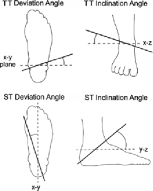
Figure 1: The deviation and inclination angles of the tibiotarsal (TT) and subtalar (ST) human ankle rotation axes.

Using an average generic orientation for each axis results in substantial errors [Lewis et al. (2009)] because of an important between subject variation in axis locations as characterized in Section 7.1 below. Several in vivo estimation methods have been proposed in biomechanical journals [see, for instance, van den Bogert, Smith and Nigg (1994) and Lewis et al. (2009)], but none was completely successful at estimating the angles in Figure 1. The poor numerical results obtained by Lewis, Sommer and Piazza (2006) led them to question the validity of the two-axis model for the ankle.

The in vivo estimation of the orientation of the two axes of the ankle is a statistical problem. The data set for one individual is a sequence of $3\times 3$ rotation matrices giving the relative orientation of the foot of the subject with respect to its lower leg as its ankle moves up and down, right and left, as much as possible. Rivest, Baillargeon and Pierrynowski (2008) and van den Bogert, Smith and Nigg (1994) provide more details about data collection.

Following van den Bogert, Smith and Nigg (1994), Rivest, Baillargeon and Pierrynowski (2008) developed a statistical model for analyzing the rotation data collected on a single ankle. Its parameters are the four angles defined in Figure 1 and a fifth one for the relative position of the two rotation axes. This model fits well; the residual standard deviations reported in Rivest, Baillargeon and Pierrynowski (2008) are around one degree. For a subject whose ankle has an average range of motion, the estimates are, however, not repeatable. Two data sets collected on the same ankle in similar conditions can give different estimated angles. This occurs because the likelihood function does not have a clear maximum; it has a plateau and some angles cannot be estimated independently of the others. Indeed, Rivest, Baillargeon and Pierrynowski (2008) demonstrate that only three parameters can be reliably estimated in a subject with an average ankle range of motion. Considering the small range of the residual angles, a failure of the two-axis model is an unlikely cause for the poor repeatability of the results.

This paper suggests methods to improve the numerical stability of the estimates derived from the ankle model. A penalized likelihood is proposed for estimating the parameters. The penalty is obtained by assuming a prior multivariate normal distribution for the five angle parameters. When the mean and the variance covariance matrix of the prior distribution are not known, one is confronted with a nonlinear mixed effects directional model whose parameters can be estimated using ankle’s data collected on a sample of volunteers. Two numerical algorithms to fit this model are proposed. Their performances are evaluated in a Monte Carlo experiment; two data sets are then analyzed using the new nonlinear mixed effects directional model.

Nonlinear mixed effects vary with the parametrization of the random effects. Thus, the first step of the analysis is to parameterize the model of Rivest, Baillargeon and Pierrynowski (2008) in terms of the angles presented in Figure 1 and to derive inference techniques using this parametrization. These procedures are then generalized to a Bayesian setting obtained by multiplying the likelihood by the prior distribution of the model parameters. The algorithms of Lindstrom and Bates (1990) [see also Pinheiro and Bates (2000)] for fitting nonlinear mixed effects models are then adapted to the new directional model.

Nonlinear mixed effects and Bayesian models with concentrated prior distributions could potentially be used in many problems of directional statistics. These techniques could, for instance, be applied to the spherical regression model considered by Kim (1991) and Bingham, Chang and Richards (1992) and to the directional one way ANOVA model of Rancourt, Rivest and Asselin (2000) to characterize the between subject variability of the mean rotation.

This new statistical methodology has important applications in biomechanics. By fitting a nonlinear mixed effects directional model to data collected on a sample of volunteers, one is able to estimate the mean values and the between subject variances of the five anatomical angles in the population. These estimates are found to be close to the clinically accepted results obtained by Inman (1976) who used direct measurements from cadaveric feet. This provides an empirical validation of the two-axis model of van den Bogert, Smith and Nigg (1994) for the ankle. The new model also allows the analysis of the rotation data collected by Pierrynowski et al. (2003) which compared the orientations of the subtalar axis of two groups of individuals classified according to their lower extremity injuries. Finally, the penalized predictions associated to the mixed effect model are shown to be more stable than the estimates obtained by maximizing the standard unpenalized likelihood for one subject.

2 Parameterization of unit vectors and of rotation matrices using anatomical angles

Let $\mathbf{A}_{1}$ and $\mathbf{B}_{2}$ be $3\times 1$ unit vectors giving the tibiotarsal and the subtalar rotation axes in a coordinate system defined according to the RFU convention. These unit vectors are first expressed in terms of the anatomical angles. Then the Cardan angle decomposition for a $3\times 3$ rotation matrix is briefly reviewed. This section uses the $\arctan$ function with two arguments, such that $\arctan(a,b)$ is the angle whose sine and cosine are given by $a/\sqrt{a^{2}+b^{2}}$ and $b/\sqrt{a^{2}+b^{2}}$, respectively.

First consider the tibiotarsal axis, $\mathbf{A}_{1}=(A_{11},A_{21},A_{31}){{}^{\top}}$, where “^⊤” denotes a matrix transpose. Formally, the anatomical angles are defined as $\mathit{ttinc}=t_{1}=-\arctan(A_{31},A_{11})$ and $\mathit{ttdev}=t_{2}=\arctan(A_{21},A_{11})$. Without loss of generality, we assume that the first coordinate of $\mathbf{A}_{1}$ is positive. A general expression for unit vectors in the half unit sphere is

$$\mathbf{A}_{1}=\frac{1}{D_{t}}\pmatrix{\cos(t_{1})\cr\cos(t_{1})\tan(t_{2})\cr-\sin(t_{1})},\qquad t_{1},t_{2}\in[-\pi/2,\pi/2),$$ (1)

where $D_{t}=\sqrt{1+\cos^{2}(t_{1})\tan^{2}(t_{2})}$. In a similar manner, one can parameterize the subtalar axis in terms of the anatomical angles $\mathit{stinc}=s_{1}=\arctan(B_{32},B_{22})$ and $\mathit{stdev}=s_{2}=-\arctan(B_{12},B_{22})$ as follows,

$$\mathbf{B}_{2}=\frac{1}{D_{s}}\pmatrix{-\cos(s_{1})\tan(s_{2})\cr\cos(s_{1})\cr\sin(s_{1})},\qquad s_{1},s_{2}\in[-\pi/2,\pi/2),$$ (2)

where $D_{s}=\sqrt{1+\cos^{2}(s_{1})\tan^{2}(s_{2})}$.

The set $\mathit{SO}(3)$ of $3\times 3$ rotation matrices is a three-dimensional manifold whose properties are reviewed in McCarthy (1990), Chirikjian and Kyatkin (2001) and León, Massé and Rivest (2006). This paper uses the Cardan angle parametrization with the $X-Z-Y$ convention. It expresses an element of $\mathit{SO}(3)$ as a function of the Cardan angles $\alpha\in[-\pi,\pi)$, $\gamma\in[-\pi/2,\pi/2)$ and $\phi\in[-\pi,\pi)$ as

$$\hskip 18.0pt\mathbf{R} = \pmatrix{1&0&0\cr 0&\cos\alpha&-\sin\alpha\cr 0&\sin\alpha&\cos\alpha}\pmatrix{\cos\gamma&-\sin\gamma&0\cr\sin\gamma&\cos\gamma&0\cr 0&0&1}\pmatrix{\cos\phi&0&\sin\phi\cr 0&1&0\cr-\sin\phi&0&\cos\phi}$$

$$= \pmatrix{\cos\gamma\cos\phi&-\sin\gamma&\cos\gamma\sin\phi\cr\cdots&\cos\alpha\cos\gamma&\cdots\cr\cdots&\sin\alpha\cos\gamma&\cdots},\!\!\!\!\!\!\!$$

where $\cdots$ stands for complex trigonometric expressions that are not used in the sequel. We also write $\mathbf{R}=\mathbf{R}(\alpha,x)\times\mathbf{R}(\gamma,z)\times\mathbf{R}(\phi,y)$, where the arguments of $\mathbf{R}(\cdot,\cdot)$ are the angle and the axis of the rotation respectively.

The model presented in the next section uses rotation matrices, $\mathbf{A}(t_{1},t_{2})$ and $\mathbf{B}(s_{1},s_{2}),$ whose first and second columns are respectively equal to $\mathbf{A}_{1}$ and $\mathbf{B}_{2}$. These matrices are given by

$$\mathbf{A}(t_{1},t_{2}) = \mathbf{R}(t_{1},y)\mathbf{R}[\arctan\{\cos(t_{1})\tan(t_{2}),1\},z]$$

$$= \frac{1}{D_{t}}\pmatrix{\cos(t_{1})&-\cos^{2}(t_{1})\tan(t_{2})&\sin(t_{1})D_{t}\cr\cos(t_{1})\tan(t_{2})&1&0\cr-\sin(t_{1})&\sin(t_{1})\cos(t_{1})\tan(t_{2})&\cos(t_{1})D_{t}}$$

and

$$\mathbf{B}(s_{1},s_{2}) = \mathbf{R}(s_{1},x)\mathbf{R}[\arctan\{\cos(s_{1})\tan(s_{2}),1\},z]$$

$$= \frac{1}{D_{s}}\pmatrix{1&-\cos(s_{1})\tan(s_{2})&0\cr\cos^{2}(s_{1})\tan(s_{2})&\cos(s_{1})&-\sin(s_{1})D_{s}\cr\sin(s_{1})\cos(s_{1})\tan(s_{2})&\sin(s_{1})&\cos(s_{1})D_{s}},$$

where $D_{t}$ and $D_{s}$ are defined in (1) and (2), respectively.

3 The model for estimating the rotation axes of a single ankle

This section expresses the model of Rivest, Baillargeon and Pierrynowski (2008) for the estimation of the anatomical angles for a single subject in terms of the rotation matrices $\mathbf{A}(t_{1},t_{2})$ and $\mathbf{B}(s_{1},s_{2})$. The data set is a sequence of time ordered $3\times 3$ rotation matrices $\{\mathbf{R}_{i}\dvtx i=1,\ldots,n\}$. The model for $\mathbf{R}_{i}$ involves the four anatomical angles, rotation angles $\{\alpha_{i}\dvtx i=1,\ldots,n\}$ and $\{\phi_{i}\dvtx i=1,\ldots,n\}$ in $[-\pi,\pi)$ about the two rotation axes and the angle $\gamma_{0}\in(-\pi/2,\pi/2)$, related to the relative position of the two axes. The predicted value $\bolds{\Psi}_{i}$ for $\mathbf{R}_{i}$ is given by

$$\bolds{\Psi}_{i}=\mathbf{A}(t_{1},t_{2})\mathbf{R}(\alpha_{i},x)\mathbf{R}(\gamma_{0},z)\mathbf{R}(\phi_{i},y)\mathbf{B}(s_{1},s_{2}){{}^{\top}}.$$ (4)

The errors are assumed to have a symmetric Fisher–von Mises matrix distribution with density $f(\mathbf{E})=\exp\{\kappa\operatorname{tr}(\mathbf{E})\}/c_{\kappa}$, $\mathbf{E}\in\mathit{SO}(3)$, where $c_{\kappa}$ is a normalizing constant; see Mardia and Jupp (2000). If the parameter $\kappa$ is assumed to be large so that the error rotations are clustered around the identity matrix $\mathbf{I}_{3}$, one has

$$\mathbf{E}=\mathbf{I}_{3}+\pmatrix{0&-\varepsilon_{3}&\varepsilon_{2}\cr\varepsilon_{3}&0&-\varepsilon_{1}\cr-\varepsilon_{2}&\varepsilon_{1}&0}+O_{p}\biggl{(}\frac{1}{\kappa}\biggr{)},$$ (5)

where the entries $\varepsilon_{1}$, $\varepsilon_{2}$, $\varepsilon_{3}$ of the skew-symmetric matrix have independent $\mathcal{N}\{0,1/(2\kappa)\}$ distributions; $1/(2\kappa)$ is called the residual variance. The model postulates that $\mathbf{R}_{i}=\bolds{\Psi}_{i}\mathbf{E}_{i}$, for $i=1,\ldots,n$. The likelihood is $L[t_{1},t_{2},s_{1},s_{2},\gamma_{0},\break\kappa,\{\alpha_{i}\},\{\phi_{i}\}]=\prod_{i}f(\bolds{\Psi}_{i}{{}^{\top}}\mathbf{R}_{i})$. Rivest, Baillargeon and Pierrynowski (2008) show that the angles $\{\alpha_{i}\}$ and $\{\phi_{i}\}$ can be profiled out of the likelihood. Indeed,

$$\qquad L[t_{1},t_{2},s_{1},s_{2},\gamma_{0},\kappa,\{\alpha_{i}\},\{\phi_{i}\}] \leq L_{p}(t_{1},t_{2},s_{1},s_{2},\gamma_{0},\kappa)$$

$$= \frac{1}{c_{\kappa}^{n}}\exp\Biggl{[}\kappa\sum_{i=1}^{n}\{2\cos(\theta_{i}^{z}-\gamma_{0})+1\}\Biggr{]},$$

where $\theta_{i}^{z}=-\arcsin(\mathbf{A}_{1}{{}^{\top}}\mathbf{R}_{i}\mathbf{B}_{2})$ is the $Z$-Cardan angle of $\mathbf{A}(t_{1},t_{2}){{}^{\top}}\mathbf{R}_{i}$ $\mathbf{B}(s_{1},s_{2})$ in the $X-Z-Y$ convention; see (2).

Several methods are available to maximize (3). However, for the implementation of the mixed effects directional model, a closed form expression for the score vector for $\bolds{\beta}=(t_{1},t_{2},s_{1},s_{2},\gamma_{0}){{}^{\top}}$ is needed. This is derived now. Observe that $\cos(\theta)=1-2\sin^{2}(\theta/2)$, where $\theta/2$ can be assumed to lie in the interval $[-\pi/2,\pi/2)$. The log profile likelihood is equal to

$$\log L_{p}(t_{1},t_{2},s_{1},s_{2},\gamma_{0},\kappa)=-4\kappa\sum_{i=1}^{n}\sin^{2}\biggl{(}\frac{\theta_{i}^{z}-\gamma_{0}}{2}\biggr{)}-n\log c_{\kappa}+3n\kappa.$$

The score for $\gamma_{0}$ is easily evaluated, viz.

$$\frac{\partial}{\partial\gamma_{0}}\log L_{p}(t_{1},t_{2},s_{1},s_{2},\gamma_{0},\kappa)=4\kappa\sum_{i=1}^{n}\sin\biggl{(}\frac{\theta_{i}^{z}-\gamma_{0}}{2}\biggr{)}\cos\biggl{(}\frac{\theta_{i}^{z}-\gamma_{0}}{2}\biggr{)}.$$

The score for the four remaining parameters involve the following partial derivatives that are evaluated using elementary methods. The property that the partial derivatives of a unit vector and the unit vector itself are orthogonal was used to get the following results:

$$\frac{\partial}{\partial t_{1}}\mathbf{A}_{1} = -\frac{\sin(t_{1})\tan(t_{2})}{D_{t}^{2}}\mathbf{A}_{2}-\frac{1}{D_{t}}\mathbf{A}_{3},$$

$$\frac{\partial}{\partial t_{2}}\mathbf{A}_{1} = \frac{\cos(t_{1})\{1+\tan^{2}(t_{2})\}}{D_{t}^{2}}\mathbf{A}_{2},$$

$$\frac{\partial}{\partial s_{1}}\mathbf{B}_{2} = \frac{\sin(s_{1})\tan(s_{2})}{D_{s}^{2}}\mathbf{B}_{1}+\frac{1}{D_{s}}\mathbf{B}_{3},$$

$$\frac{\partial}{\partial s_{2}}\mathbf{B}_{2} = -\frac{\cos s_{1}\{1+\tan^{2}(s_{2})\}}{D_{s}^{2}}\mathbf{B}_{1}.$$

Since $\theta_{i}^{z}=-\arcsin(\mathbf{A}_{1}{{}^{\top}}\mathbf{R}_{i}\mathbf{B}_{2})$, the score for $t_{1}$ is given by

$$\frac{\partial}{\partial t_{1}}\log L_{p}(t_{1},t_{2},s_{1},s_{2},\gamma_{0},\kappa) = -4\kappa\sum_{i=1}^{n}\sin\biggl{(}\frac{\theta_{i}^{z}-\gamma_{0}}{2}\biggr{)}\cos\biggl{(}\frac{\theta_{i}^{z}-\gamma_{0}}{2}\biggr{)}$$

$$\hphantom{-4\kappa\sum_{i=1}^{n}}{}\times\frac{-1}{\sqrt{1-(\mathbf{A}_{1}{{}^{\top}}\mathbf{R}_{i}\mathbf{B}_{2})^{2}}}\frac{\partial}{\partial t_{1}}\mathbf{A}_{1}{{}^{\top}}\mathbf{R}_{i}\mathbf{B}_{2}.$$

This can be evaluated using the previous expressions for the partial derivatives. Repeating this for the other anatomical angles leads to

$$\frac{\partial}{\partial\bolds{\beta}}\log L_{p}(\beta,\kappa) = -4\kappa\sum_{i=1}^{n}\sin\biggl{(}\frac{\theta_{i}^{z}-\gamma_{0}}{2}\biggr{)}\cos\biggl{(}\frac{\theta_{i}^{z}-\gamma_{0}}{2}\biggr{)}\frac{\partial}{\partial\bolds{\beta}}(\theta_{i}^{z}-\gamma_{0})$$

$$= -4\kappa\sum_{i=1}^{n}\sin\biggl{(}\frac{\theta_{i}^{z}-\gamma_{0}}{2}\biggr{)}\mathbf{X}_{i},$$

where

$$\mathbf{X}_{i} = -\frac{\cos\{(\theta_{i}^{z}-\gamma_{0})/2\}}{\sqrt{1-(\mathbf{A}_{1}{{}^{\top}}\mathbf{R}_{i}\mathbf{B}_{2})^{2}}}$$

$$\phantom{-}{}\times\pmatrix{\displaystyle-\frac{\sin(t_{1})\tan(t_{2})}{D_{t}^{2}}\mathbf{A}_{2}{{}^{\top}}\mathbf{R}_{i}\mathbf{B}_{2}-\frac{1}{D_{t}}\mathbf{A}_{3}{{}^{\top}}\mathbf{R}_{i}\mathbf{B}_{2}\cr\displaystyle\frac{\cos(t_{1})\{1+\tan^{2}(t_{2})\}}{D_{t}^{2}}\mathbf{A}_{2}{{}^{\top}}\mathbf{R}_{i}\mathbf{B}_{2}\cr\displaystyle\frac{\sin(s_{1})\tan(s_{2})}{D_{s}^{2}}\mathbf{A}_{1}{{}^{\top}}\mathbf{R}_{i}\mathbf{B}_{1}+\frac{1}{D_{s}}\mathbf{A}_{1}{{}^{\top}}\mathbf{R}_{i}\mathbf{B}_{3}\cr\displaystyle-\frac{\cos(s_{1})\{1+\tan^{2}(s_{2})\}}{D_{s}^{2}}\mathbf{A}_{1}{{}^{\top}}\mathbf{R}_{i}\mathbf{B}_{1}\cr\sqrt{1-(\mathbf{A}_{1}{{}^{\top}}\mathbf{R}_{i}\mathbf{B}_{2})^{2}}}.$$

Evaluated at $\bolds{\beta}+\delta(\bolds{\beta})$, where $\delta(\bolds{\beta})$ is a $5\times 1$ vector with entries close to 0, the score vector (3) is

$$-4\kappa\sum_{i=1}^{n}\biggl{\{}\sin\biggl{(}\frac{\theta_{i}^{z}-\gamma_{0}}{2}\biggr{)}\mathbf{X}_{i}+\frac{1}{2}\mathbf{X}_{i}\mathbf{X}_{i}{{}^{\top}}\delta(\bolds{\beta})\biggr{\}}$$

$$\qquad{}+O(\|\delta(\bolds{\beta})\|^{2})+O\bigl{(}\max[|\sin\{(\theta_{i}^{z}-\gamma_{0})/2\}|\|\delta(\bolds{\beta})\|]\bigr{)}.$$

One can consider that the last two terms are negligible since the residuals $(\theta_{i}^{z}-\gamma_{0})$ are small. This is standard in the large $\kappa$ asymptotics used to approximate the sampling distributions of estimators in a directional model: both $\hat{\bolds{\beta}}-\bolds{\beta}$ and the errors $\varepsilon_{j}$ in (5) are assumed to be $O(1/\sqrt{\kappa})$; see, for instance, Rivest and Chang (2006). Equating this to 0 yields a simple updating formula. Given its current value $\bolds{\beta}$, the updated value is $\bolds{\beta}+\delta(\bolds{\beta})$, where

$$\delta(\bolds{\beta})=-\Biggl{(}\sum_{i=1}^{n}\mathbf{X}_{i}\mathbf{X}_{i}{{}^{\top}}\Biggr{)}^{-1}\sum_{i=1}^{n}\biggl{\{}2\sin\biggl{(}\frac{\theta_{i}^{z}-\gamma_{0}}{2}\biggr{)}\mathbf{X}_{i}\biggr{\}}.$$

This calculation can be carried out by regressing the residual vector $[2\sin\{(\theta_{i}^{z}-\gamma_{0})/2\}]$ on the explanatory variables $\{\mathbf{X}_{i}\}$. Theorem 1 of Rivest, Baillargeon and Pierrynowski (2008) holds and, as $\kappa$ goes to $\infty$, the maximum likelihood estimator $\hat{\bolds{\beta}}$ is approximately normally distributed. Once the model is fitted, the residual variance $1/(2\kappa)$ can be estimated using the sum of the squared residuals,

$$\frac{1}{2\hat{\kappa}}=\frac{1}{n}\sum_{i=1}^{n}4\sin^{2}\{(\hat{\theta}_{i}^{z}-\hat{\gamma}_{0})/2\},$$

where the residual angle $\hat{\theta}_{i}^{z}=-\arcsin(\widehat{\mathbf{A}}_{1}{{}^{\top}}\mathbf{R}_{i}\widehat{\mathbf{B}}_{2})$ is the $Z$-Cardan angle of $\widehat{\mathbf{A}}{{}^{\top}}\mathbf{R}_{i}\widehat{\mathbf{B}}$ in the $X-Z-Y$ convention. Using Grood and Suntay (1983) clinical interpretation, rotations of angle $\{\hat{\theta}_{i}^{z}\}$ occur about a floating axis that is orthogonal to both the $\mathit{tt}$ and the $\mathit{st}$ axes. Plots of these angles appear in Figure 2 of Rivest, Baillargeon and Pierrynowski (2008); their residual standard deviation, $\sqrt{1/2\hat{\kappa}}$, is about one degree. The distribution of the residuals $\{[2\sin\{(\theta_{i}^{z}-\gamma_{0})/2\}]\}$ is usually approximately normal; the normality assumption in (5) is not violated for most of the data sets investigated. Thus, the proposed model fits well to the ankle data.

Many individuals have a limited ankle range of motion; the domains for angles $\{\alpha_{i}\}$ and $\{\phi_{i}\}$ in (4) are therefore limited. This makes the estimates of the anatomical angles numerically unstable. There can be important differences between the estimates calculated on two data sets collected in succession on the same ankle; see Rivest, Baillargeon and Pierrynowski (2008). Thus, individual measurements do not allow the estimation of a complete set of anatomical angles. This suggests to borrow strength from other individuals and to consider a Bayesian model whose prior distribution penalizes extreme parameter values.

4 A Bayesian ankle model

Assume, for now, that the residual variance $1/(2\kappa)$ is known and that the $5\times 1$ vector of anatomical angles $\bolds{\beta}$ is random and has a $\mathcal{N}_{5}(\bolds{\beta}_{0},\bolds{\Sigma}_{0})$, where $\bolds{\beta}_{0}$ is the average vector of anatomical angles within the population and the $5\times 5$ variance covariance matrix $\bolds{\Sigma}_{0}$ characterizes the variability of the anatomical angles within the population; both are assumed to be known. Elements of $\bolds{\beta}_{0}$ and $\bolds{\Sigma}_{0}$ could be set equal to the values of Inman (1976), who studied the variability of these angles. We assume that $\bolds{\Sigma}_{0}$ is $O(1/(2\kappa))$, thus, there is a fixed $5\times 5$ upper triangular matrix $\bolds{\Delta}_{0}$ such that $\bolds{\Sigma}_{0}=\bolds{\Delta}_{0}^{-1}(\bolds{\Delta}_{0}^{-\top})/(2\kappa)$, where $\bolds{\Delta}_{0}^{-\top}$ is the inverse of $\bolds{\Delta}_{0}^{\top}$. This section presents an algorithm to derive the mode of the posterior distribution of $\bolds{\beta}$ and suggests an approximation for its posterior distribution.

The posterior distribution of $\bolds{\beta}$ is proportional to

$$\exp\Biggl{[}-\kappa\Biggl{\{}\sum_{i=1}^{n}4\sin^{2}\biggl{(}\frac{\theta_{i}^{z}-\gamma_{0}}{2}\biggr{)}+(\bolds{\beta}-\bolds{\beta}_{0}){{}^{\top}}\Delta_{0}{{}^{\top}}\Delta_{0}(\bolds{\beta}-\bolds{\beta}_{0})\Biggr{\}}\Biggr{]}$$

$$\qquad=\exp\{-\kappa\mathit{SSE}(\bolds{\beta})\}.$$

The posterior mode $\widehat{\bolds{\beta}}$ is the value of $\bolds{\beta}$ that minimizes $\mathit{SSE}$. It can be evaluated by adapting the regression algorithm of Section 3 to the Bayesian framework. The vector of partial derivatives of $\mathit{SSE}$ with respect to $\bolds{\beta}$ is easily derived,

$$\frac{\partial}{\partial\bolds{\beta}}\mathit{SSE}(\bolds{\beta})=4\sum_{i=1}^{n}\sin\biggl{(}\frac{\theta_{i}^{z}-\gamma_{0}}{2}\biggr{)}\mathbf{X}_{i}+2\Delta_{0}{{}^{\top}}\Delta_{0}(\bolds{\beta}-\bolds{\beta}_{0}),$$ (9)

where the vector of partial derivatives $\mathbf{X}_{i}$ is defined by (3).

Proceeding as in Section 3, one constructs an algorithm for minimizing $\mathit{SSE}$. The current value $\bolds{\beta}$ is updated to $\bolds{\beta}+\delta(\bolds{\beta})$, where

$$\delta(\bolds{\beta})=-\Biggl{(}\sum_{i=1}^{n}\mathbf{X}_{i}\mathbf{X}_{i}{{}^{\top}}+\Delta_{0}{{}^{\top}}\Delta_{0}\Biggr{)}^{-1}\Biggl{[}\sum_{i=1}^{n}\biggl{\{}2\sin\biggl{(}\frac{\theta_{i}^{z}-\gamma_{0}}{2}\biggr{)}\mathbf{X}_{i}\biggr{\}}$$

$$\hskip 182.0pt{}+\Delta_{0}{{}^{\top}}\Delta_{0}(\bolds{\beta}-\bolds{\beta}_{0})\Biggr{]}.$$

An alternative expression for the updated value is

$$\bolds{\beta}+\delta(\bolds{\beta}) = \Biggl{(}\sum_{i=1}^{n}\mathbf{X}_{i}\mathbf{X}_{i}{{}^{\top}}+\Delta_{0}{{}^{\top}}\Delta_{0}\Biggr{)}^{-1}$$

$${}\times\Biggl{[}\sum_{i=1}^{n}\biggl{\{}-2\sin\biggl{(}\frac{\theta_{i}^{z}-\gamma_{0}}{2}\biggr{)}+\mathbf{X}_{i}{{}^{\top}}\bolds{\beta}\biggr{\}}\mathbf{X}_{i}+\Delta_{0}{{}^{\top}}\Delta_{0}\bolds{\beta}_{0}\Biggr{]}.$$

An approximation to the posterior distribution of the anatomical angles is given next.

Proposition 1

As $\kappa\to\infty$, the posterior distribution for $\beta$ satisfies

$$\sqrt{2\kappa}(\bolds{\beta}-\hat{\bolds{\beta}})\sim\mathcal{N}_{5}\Biggl{\{}0,\Biggl{(}\sum_{i=1}^{n}\hat{\mathbf{X}}_{i}\hat{\mathbf{X}}_{i}{{}^{\top}}+\Delta_{0}{{}^{\top}}\Delta_{0}\Biggr{)}^{-1}\Biggr{\}},$$

where $\hat{\mathbf{X}}_{i}$ denotes the $5\times 1$ vector of partial derivatives defined by (3) and evaluated at $\hat{\bolds{\beta}}$.

The posterior density of $\delta=\sqrt{2\kappa}(\bolds{\beta}-\hat{\bolds{\beta}})$ is proportional to $\exp\{-\kappa\mathit{SSE}(\hat{\bolds{\beta}}+\delta/\sqrt{2\kappa})\}$. The result is proved by taking a second-order Taylor series expansion around $\delta=0$. The first order derivatives are null and the variance covariance matrix of Proposition 1 is obtained by dropping the $o\{1/(2\kappa)\}$ terms in the matrix of second-order derivatives.

We now study some frequentist properties of $\hat{\bolds{\beta}}$. Let $\bolds{\beta}^{(t)}$ be the true values of the anatomical angles for the individual under consideration. Thus, $\bolds{\beta}^{(t)}$ is a realization of the $\mathcal{N}_{5}(\bolds{\beta}_{0},\bolds{\Sigma}_{0})$ prior distribution, such that $\|\bolds{\beta}^{(t)}-\bolds{\beta}_{0}\|$ is $O(1/\sqrt{2\kappa})$. The difference $\hat{\bolds{\beta}}-\bolds{\beta}^{(t)}$ is $O(1/\sqrt{2\kappa})$. The leading term of this difference consists of a linear combination of individual experimental errors and of the penalty associated to the prior distribution. To get a closed form expression, one can proceed as in Appendix B of Rivest, Baillargeon and Pierrynowski (2008). It suffices to carry out a first-order Taylor series expansion of (9) in terms of the difference $\delta(\bolds{\beta})={\bolds{\beta}}-\bolds{\beta}^{(t)}$ and of the experimental errors. This yields

$$\frac{\partial}{\partial\bolds{\beta}}\mathit{SSE}\bigl{(}\bolds{\beta}^{(t)}+\delta(\bolds{\beta})\bigr{)}$$

$$\qquad=2\Biggl{\{}\sum_{i=1}^{n}\epsilon_{i}\mathbf{X}_{i}^{(t)}+\sum_{i=1}^{n}\mathbf{X}_{i}^{(t)}\mathbf{X}_{i}^{(t)T}\delta(\bolds{\beta})+\Delta_{0}{{}^{\top}}\Delta_{0}\bigl{(}\delta(\bolds{\beta})+\bolds{\beta}^{(t)}-\bolds{\beta}_{0}\bigr{)}\Biggr{\}}$$ (10)

$$\qquad\quad{}+O(1/\kappa),$$

where $\epsilon_{i}$ is a $\mathcal{N}(0,1/(2\kappa))$ random variable that depends on the error matrix $\mathbf{E}_{i}$, and $\mathbf{X}_{i}^{(t)}$ denotes the vector of partial derivatives $\mathbf{X}_{i}$ evaluated at the true value $\bolds{\beta}^{(t)}$, with $R_{i}$ set equal to $\Psi_{i}$ in (3). Now $\hat{\bolds{\beta}}$ corresponds to the value of $\delta(\bolds{\beta})$ for which (4) is null, thus,

$$\hat{\bolds{\beta}} = \bolds{\beta}^{(t)}-\Biggl{(}\sum_{i=1}^{n}\mathbf{X}_{i}^{(t)}\mathbf{X}_{i}^{(t)T}+\bolds{\Delta}_{0}{{}^{\top}}\bolds{\Delta}_{0}\Biggr{)}^{-1}$$

$$\hphantom{\bolds{\beta}^{(t)}-\,}{}\times\Biggl{\{}\sum_{i=1}^{n}\epsilon_{i}\mathbf{X}_{i}^{(t)}+\bolds{\Delta}_{0}{{}^{\top}}\bolds{\Delta}_{0}\bigl{(}\bolds{\beta}^{(t)}-\bolds{\beta}_{0}\bigr{)}\Biggr{\}}+O(1/\kappa)$$

$$= \Biggl{(}\sum_{i=1}^{n}\mathbf{X}_{i}^{(t)}\mathbf{X}_{i}^{(t)T}+\bolds{\Delta}_{0}{{}^{\top}}\bolds{\Delta}_{0}\Biggr{)}^{-1}$$

$${}\times\Biggl{\{}\sum_{i=1}^{n}\bigl{(}\mathbf{X}_{i}^{(t)T}\bolds{\beta}^{(t)}-\epsilon_{i}\bigr{)}\mathbf{X}_{i}^{(t)}+\bolds{\Delta}_{0}{{}^{\top}}\bolds{\Delta}_{0}\bolds{\beta}_{0}\Biggr{\}}+O(1/\kappa).$$

This expansion provides an approximation for the prediction error of $\hat{\bolds{\beta}}$ as a predictor of $\bolds{\beta}^{(t)}$. The posterior variance covariance matrix of $\bolds{\beta}^{(t)}$ given in Proposition 1 is an estimate of the variance covariance matrix of the approximate prediction error.

5 A mixed model for the simultaneous estimation of several sets of anatomical angles

We now have $M$ subjects and $n_{i}$, $1\leq i\leq M$, observed rotation matrices on each subject. The data set consists of the $3\times 3$ rotation matrices $\{\mathbf{R}_{ij}\dvtx i=1,\ldots,M;j=1,\ldots,n_{i}\}$. Let $\bolds{\beta}_{i}=(t_{1i},t_{2i},s_{1i},s_{2i},\gamma_{0i}){{}^{\top}}$ be the anatomical angles for the $i$th ankle. As in Section 4, the angles $\bolds{\beta_{i}}$ are assumed to be random deviates with a five-dimensional normal distribution, $\mathcal{N}_{5}(\bolds{\beta}_{0},\bolds{\Sigma}_{0})$. The fixed parameters $\kappa$, $\bolds{\beta}_{0}$ and $\bolds{\Sigma}_{0}$ are assumed to be unknown.

In a mixed effects model, the fixed regression parameters and the variance components are estimated using a marginal likelihood. To estimate $\bolds{\beta}_{0}$ and $\bolds{\Sigma}_{0}$, we construct such a likelihood using the profile likelihood defined in (3), rather than the full likelihood for the ankle model. This is acceptable since this profile likelihood is also a likelihood, constructed by assuming that the angles $\theta_{ij}^{z}-\gamma_{0i}$ defined in (3) have a centered angular von Mises distribution with shape parameter $2\kappa$. Indeed, since $\kappa$ is large, the distribution of $2\sin\{(\theta_{ij}^{z}-\gamma_{0i})/2\}$ is approximately $\mathcal{N}\{0,1/(2\kappa)\}$. Using this approximation in the evaluation of the marginal likelihood $L_{1p}$ gives

$$\prod_{i=1}^{M}\biggl{(}\frac{\kappa}{\pi}\biggr{)}^{(n_{i}+5)/2}|\bolds{\Delta}_{0}|$$

(11)

$$\qquad{}\times\int_{\mathbb{R}^{5}}\exp\Biggl{\{}-\kappa\sum_{j=1}^{n_{i}}4\sin^{2}\biggl{(}\frac{\theta_{ij}^{z}-\gamma_{0i}}{2}\biggr{)}-\kappa\|\Delta_{0}(\bolds{\beta}_{i}-\bolds{\beta}_{0})\|^{2}\Biggr{\}}\,{\mathrm{d}}\bolds{\beta}_{i}.$$

Because of a highly nonlinear integrand, the above expression cannot be evaluated explicitly. To find the maximum value numerically, we adapt the algorithm of Lindstrom and Bates (1990) to the directional ankle model.

For each $i$, and for fixed $(\bolds{\beta}_{0},\bolds{\Delta}_{0})$, the integrand of (5) is maximized using the method presented in Section 3. Let $\hat{\bolds{\beta}}_{i}$ be the maximum value for the $i$th sample. Using the first order Taylor series expansion derived in Section 3 leads to the following approximation:

$$2\sin\biggl{(}\frac{\theta_{ij}^{z}-\gamma_{0i}}{2}\biggr{)}\approx 2\sin\biggl{(}\frac{\hat{\theta}_{ij}^{z}-\hat{\gamma}_{0i}}{2}\biggr{)}+\mathbf{X}_{ij}{{}^{\top}}({\bolds{\beta}}_{i}-\hat{\bolds{\beta}}_{i}),$$

where the angles $\hat{\theta}_{ij}^{z}$ and $\hat{\gamma}_{0i}$ and the $5\times 1$ vector of partial derivatives $\mathbf{X}_{ij}$ are evaluated at $\hat{\bolds{\beta}}_{i}$. Using this approximation, and changing variables $\bolds{\beta}_{i}-\bolds{\beta}_{0}=\mathbf{z}$ in the integral, (5) becomes

$$L_{1p} \approx \prod_{i=1}^{M}\biggl{(}\frac{\kappa}{\pi}\biggr{)}^{(n_{i}+5)/2}|\bolds{\Delta}_{0}|$$

$$\hphantom{\prod_{i=1}^{M}}{}\times\int_{\mathbb{R}^{5}}\exp\Biggl{\{}-\kappa\sum_{j=1}^{n_{i}}(\mathbf{y}_{ij}-\mathbf{X}_{ij}{{}^{\top}}{\mathbf{z}-\mathbf{X}_{ij}{{}^{\top}}\bolds{\beta}}_{0})^{2}-\kappa\|\bolds{\Delta}_{0}\mathbf{z}\|^{2}\Biggr{\}}\,{\mathrm{d}}\mathbf{z},$$

$$= \prod_{i=1}^{M}\frac{(\kappa/\pi)^{n_{i}/2}}{|\mathbf{I}+\mathbf{X}_{i}\bolds{\Delta}_{0}^{-1}\bolds{\Delta}_{0}^{-\top}\mathbf{X}_{i}{{}^{\top}}|^{1/2}}$$

$$\hphantom{\prod_{i=1}^{M}}{}\times\exp\{-\kappa(\mathbf{y}_{i}-\mathbf{X}_{i}{\bolds{\beta}}_{0}){{}^{\top}}(\mathbf{I}+\mathbf{X}_{i}\bolds{\Delta}_{0}^{-1}\bolds{\Delta}_{0}^{-\top}\mathbf{X}_{i}{{}^{\top}})^{-1}(\mathbf{y}_{i}-\mathbf{X}_{i}{\bolds{\beta}}_{0})\},$$

where $\mathbf{X}_{i}$ is the $n_{i}\times 5$ matrix of partial derivatives for the $i$th unit, and $\mathbf{y}_{i}$ is the $n_{i}\times 1$ vector whose $j$ entry is given by $\mathbf{X}_{ij}{{}^{\top}}\hat{\bolds{\beta}}_{i}-2\sin\{(\hat{\theta}_{ij}^{z}-\hat{\gamma}_{0i})/2\}$. This evaluation of the integral with respect to $\mathbf{z}$ follows the argument presented in Pinheiro and Bates (2000), Section 7.2. It involves the five-dimensional normal density with mean vector $(\mathbf{X}_{i}{{}^{\top}}\mathbf{X}_{i}+\bolds{\Delta}_{0}{{}^{\top}}\bolds{\Delta}_{0})^{-1}\mathbf{X}_{i}{{}^{\top}}(\mathbf{y}_{i}-\mathbf{X}_{i}{\bolds{\beta}}_{0})$ and variance covariance matrix equal to $(\mathbf{X}_{i}{{}^{\top}}\mathbf{X}_{i}+\bolds{\Delta}_{0}{{}^{\top}}\bolds{\Delta}_{0})^{-1}/(2\kappa)$. Thus, $L_{1p}$ is approximately equal to the likelihood function for the following linear mixed effects model:

$$\mathbf{y}=\pmatrix{\mathbf{X}_{1}\cr\vdots\cr\mathbf{X}_{M}}\bolds{\beta}_{0}+\pmatrix{\mathbf{X}_{1}&\mathbf{0}&\cdots&\mathbf{0}\cr\mathbf{0}&\mathbf{X}_{2}&\cdots&\mathbf{0}\cr\cdots&\cdots&\cdots&\cdots\cr\mathbf{0}&\mathbf{0}&\cdots&\mathbf{X}_{M}}\mathbf{b}+\bolds{\epsilon},$$ (12)

where $\mathbf{y}$ is the $(\sum n_{i})\times 1$ vector of the dependent variable, $\bolds{\beta}_{0}$ is the mean vector of the anatomical angles in the population, and $\mathbf{b}$ is the $5M\times 1$ vector of the individual random effects $\mathbf{b}_{i}=\bolds{\beta}_{i}-\bolds{\beta}_{0}$ that are assumed to be independent random vectors with a $\mathcal{N}_{5}(0,\bolds{\Sigma}_{0})$ distribution. Finally, $\bolds{\epsilon}$ is the $(\sum n_{i})\times 1$ vector of the experimental errors of the directional model containing independent $\mathcal{N}(0,1/(2\kappa))$ random deviates. The second step of the algorithm estimates $\bolds{\beta}_{0}$, $1/(2\kappa)$ and $\bolds{\Sigma}_{0}$ by fitting the linear mixed effects model (12). This gives updated values for the parameters of the prior distribution that are used to get a new set of penalized estimates $\{\hat{\bolds{\beta}}_{i}\}$; these new estimates are used to get a new approximation to (5) and to update the marginal parameter values by fitting (12). This two-step algorithm typically converges after a few iterations. It is called the PLME algorithm since it uses a Penalized least squares and an algorithm for fitting Linear Mixed Effects models. Lindstrom and Bates (1990) showed that the first step can be bypassed by using $\hat{\bolds{\beta}}_{i}^{k}=\bolds{\beta}_{0}^{k}+\mathbf{b}_{i}^{k}$ as the values around which the linearization of (5) is carried out at iteration $k+1$, where $\mathbf{b}_{i}^{k}$ is the estimate of the random effect for the $i$th individual at the $k$th iteration. This one-step algorithm is labeled LME.

This section has considered the one-sample problem, where all the individuals share the same fixed effect vector $\bolds{\beta}_{0}$. Section 7 considers a two-sample model where the direction of the subtalar axis is allowed to vary between samples. The directional mixed effects model for this problem is easily constructed. The local linear mixed effects model at step 2 of the Lindstrom and Bates (1990) algorithm has a $7\times 1$ vector of fixed regression parameters featuring 5 entries for the mean angles in the first sample and two parameters for the between group differences of the two subtalar angles. The two algorithms proposed in this section can be used to estimate the parameters of this enlarged model.

6 A simulation study

This section reports the results of a Monte Carlo experiment to investigate the sampling properties of the estimators of $\bolds{\beta}_{0}$ and $\bolds{\Sigma}_{0}$ obtained by maximizing (5) with the two versions of the Lindstrom and Bates (1990) algorithm. First, the method used to simulate the data is reviewed, then some results will be presented. In the simulations the calculations are carried out with angles expressed in radians; for convenience the results are presented in degrees.

Simulations were carried out for the one-sample model only. Values of $M=30,50,100$ and $n=50,100,200$ were considered. The simulation used 500 Monte Carlo samples. The following parameter values were used:

$$\bolds{\beta}_{0} = (8,-6,42,23,17){{}^{\top}},\qquad\bolds{\Sigma}_{0}=\operatorname{diag}(7,4,9,11,11)^{2},$$

$$1/(2\kappa) = 1.$$

The mean and standard deviations for the first four anatomical angles are as given by Inman (1976). The residual standard error $1/\sqrt{2\kappa}$ of one degree was similar to estimates found in the numerical examples of Rivest, Baillargeon and Pierrynowski (2008).

For each individual, the five anatomical angles were first simulated from a $\mathcal{N}_{5}(\bolds{\beta}_{0},\bolds{\Sigma}_{0})$ and the rotation matrices $\mathbf{A}(t_{1},t_{2})$ and $\mathbf{B}(s_{1},s_{2})$ were evaluated. To construct the predicted values $\Psi_{ij}$ given in (4), angles $(\alpha_{ij},\phi_{ij})$ obtained by fitting the one subject model to some real data were used. The average values for $(\alpha_{ij},\phi_{ij})$ were $(38,14)$ with standard deviations of $(12,10.5)$. Thus, the motion about the $\mathit{st}$ axis has a smaller range than that about the $\mathit{tt}$ axis. The rotation errors $\mathbf{E}_{ij}$ were generated from $\mathbf{z}=(z_{1},z_{2},z_{3}){{}^{\top}}$ three independent $\mathcal{N}(0,0.017^{2})$ random variables (a standard deviation of 0.017 radian is 1 when expressed in degrees). Its rotation axis was set to $\mathbf{z}/\|\mathbf{z}\|$, while its rotation angle was equal to $\|\mathbf{z}\|$. To understand the numerical challenges associated to the maximization of the likelihood for the model of Section 3, it is convenient to evaluate the vector of partial derivatives $\mathbf{X}_{ij}$ at $\bolds{\beta}=\bolds{\beta}_{0}$ in an error free model. One gets $\mathbf{X}_{ij}=(0.01\cos(\alpha_{ij})-0.99\sin(\alpha_{ij})$, $0.99\cos(\alpha_{ij})$, $0.26\cos(\phi_{ij})+0.95\sin(\phi_{ij})$, $-0.80\cos(\phi_{ij}),1){{}^{\top}}$. The matrix $\mathbf{X}_{i}$ of the vectors of partial derivatives for one subject has a condition number larger than 100. This multi-collinearity affects especially $\mathit{ttdev}$, $\mathit{stdev}$ and $\gamma_{0}$, three rotation angles about different $z$-axes that are not well differentiated when the ankle exhibits a small range of motion.

The simulations compared the two algorithms proposed by Lindstrom and Bates (1990), PLME and LME, as described in Section 5. The R-function lme was used to fit a linear mixed effects model at step 2 of the PLME algorithm. This function provides estimates of the sampling variances for the fixed effects. The biases of these variance estimators were also investigated in the Monte Carlo study. The two algorithms gave almost the same results. Only those obtained with PLME are presented.

= $\bolds n$ $\bolds M$ $\bolds s_{\mathbf{1}}$ $\bolds s_{\mathbf{2}}$ $\bolds\gamma_{\mathbf{0}}$ $\bolds t_{\mathbf{1}}$ $\bolds t_{\mathbf{2}}$ 50 230 $-0.09$ $(1.70,-2)$ $0.67$ $(3.10,-16)$ $0.55$ $(3.27,-14)$ $-$$0.10$ $(1.56,-12)$ $-0.09$ $(1.26,-14)$ 50 250 $-0.17$ $(1.34,-4)$ $0.74$ $(2.44,-13)$ $0.54$ $(2.74,-19)$ $-$$0.03$ $(1.14,-2)$ $-0.06$ $(0.99,-12)$ 50 100 $-0.13$ $(0.97,-9)$ $0.85$ $(1.91,-33)$ $0.68$ $(1.96,-23)$ $-$$0.05$ $(0.85,-12)$ $-0.12$ $(0.73,-17)$ 100 230 $-0.09$ $(1.58,11)$ $0.26$ $(2.69,-10)$ $0.22$ $(2.92,-13)$ $-$$0.02$ $(1.37,0)$ $-$$0.04$ $(1.09,-7)$ 100 250 $-0.08$ $(1.28,4)$ $0.52$ $(2.13,-11)$ $0.24$ $(2.17,-4)$ $-$$0.06$ $(1.06,2)$ $-0.03$ $(0.79,0)$ 100 100 $-0.07$ $(0.90,4)$ $0.42$ $(1.52,-14)$ $0.30$ $(1.63,-17)$ $-0.09$ $(0.79,-8)$ $-0.02$ $(0.58,-9)$ 200 230 $-0.01$ $(1.70,-5)$ $0.16$ $(2.34,-3)$ $0.06$ $(2.50,-9)$ $-$$0.06$ $(1.38,-7)$ $-$$0.05$ $(0.86,9)$ 200 250 $-0.09$ $(1.32,-5)$ $0.39$ $(1.87,-6)$ $0.27$ $(1.96,-8)$ $-0.02$ $(1.03,0)$ $-$$0.00$ $(0.65,13)$ 200 100 $-0.06$ $(0.89,4)$ $0.21$ $(1.34,-9)$ $0.06$ $(1.44,-15)$ $-0.01$ $(0.75,-5)$ $-$$0.05$ $(0.53,-13)$ $\bolds n$ $\bolds M$ $\bolds{\sigma_{t_{1}}}$ $\bolds{\sigma_{t_{2}}}$ $\bolds{\sigma_{s_{1}}}$ $\bolds{\sigma_{s_{2}}}$ $\bolds{\sigma_{\gamma_{0}}}$ 50 130 $-0.05$ $(1.10)$ $-0.28$ $(1.28)$ $-0.19$ $(1.25)$ $-0.04$ $(2.34)$ $-0.46$ $(2.50)$ 50 150 $-0.06$ $(0.78)$ $-0.16$ $(0.89)$ $-0.12$ $(0.99)$ $-0.02$ $(1.74)$ $-0.18$ $(1.94)$ 50 100 $-$$0.00$ $(0.53)$ $-0.07$ $(0.63)$ $-0.05$ $(0.66)$ $-$$0.03$ $(1.27)$ $-0.10$ $(1.26)$ 100 130 $-0.11$ $(0.98)$ $-0.11$ $(0.97)$ $-0.07$ $(1.21)$ $-0.14$ $(2.09)$ $-0.16$ $(2.27$) 100 150 $-$$0.00$ $(0.75)$ $-0.01$ $(0.67)$ $-0.06$ $(0.92)$ $-$$0.13$ $(1.45)$ $-0.02$ $(1.66)$ 100 100 $-0.04$ $(0.54)$ $-0.03$ $(0.49)$ $-0.05$ $(0.70)$ $-0.02$ $(1.12)$ $-0.15$ $(1.20)$ 200 130 $-0.09$ $(0.96)$ $-0.06$ $(0.76)$ $-0.09$ $(1.14)$ $-0.18$ $(1.82)$ $-0.29$ $(1.95)$ 200 150 $-0.05$ $(0.75)$ $-0.06$ $(0.58)$ $-0.07$ $(0.92)$ $-0.02$ $(1.40)$ $-0.12$ $(1.51)$ 200 100 $-0.04$ $(0.54)$ $-0.06$ $(0.41)$ $0$ $(0.68)$ $-$$0.03$ $(0.97)$ $-0.05$ $(1.07)$

Table 1: Bias and root mean squared error, in parenthesis, of the estimator of $\bolds{\beta}_{0}$ and the relative bias of the lme variance estimator, in parenthesis, when the fitted model assumes that $\bolds{\Sigma}_{0}$ is diagonal

Table 2: Biases and root mean squared errors, in parenthesis, of the estimators of the standard deviations, $\operatorname{diag}(\bolds{\Sigma}_{0}^{1/2})$,when the fitted model assumes that $\bolds{\Sigma_{0}}$ is diagonal

Tables 2 and 2 report findings where the fitted model has a diagonal $\bolds{\Sigma}_{0}$. In Table 2, the estimates for $t_{1}$, $t_{2}$ and $s_{1}$ have small biases, not significantly different from 0, and small root mean squared errors. The estimates for $s_{2}$ and $\gamma_{0}$ are less precise. This is caused by the multi-collinearity problem mentioned above. The lme variance estimates underestimate the true variances; this underestimation is more severe for the angles $s_{2}$, $t_{2}$ and $\gamma_{0}$. Increasing $n$, the number of data points by subject reduces this bias. Table 2 is concerned with the estimation of the standard deviations. It shows small negative biases for all the variances. The parameters $\sigma_{s_{2}}$ and $\sigma_{\gamma_{0}}$ have the largest root mean squared errors. Still, Tables 2 and 2 show that the directional mixed effects model gives reliable estimates when the random effects are assumed to be independent.

It is likely for the anatomical angles to be correlated so that the true value of $\bolds{\Sigma}_{0}$ might not be diagonal. Inman (1976) did not consider this question; he did not report the correlations between anatomical angles. One could investigate this problem by fitting a model with an unstructured $\bolds{\Sigma}_{0}$ with 15 parameters (that is the variances of the 5 angles and the 10 covariances between pairs of angles). Unfortunately, the results obtained with such a model are not reliable. In simulations, not reported here, biased estimates of the off-diagonal elements of $\bolds{\Sigma}_{0}$ were obtained, especially for the covariances involving $t_{2}$, $s_{2}$ and $\gamma_{0}$. Apparently, the nonlinear mixed effects model cannot distinguish a true correlation between random effects in the population from a correlation caused by an ill-conditioned likelihood for the estimation of the random effects. Additional investigations of this problem could consider models where $\bolds{\Sigma}_{0}$ has a small number of nonnull covariances.

7 Numerical examples

This section presents the analysis of two data sets collected in the Human Movement Laboratory of the School of Rehabilitation Science at McMaster University, using an OptoTrak camera system at a frequency of 50 Hz; see Rivest, Baillargeon and Pierrynowski (2008) for a detailed description of the data collection protocol. The successive rotation matrices in a data set are not independent measurements; the residual autocorrelation when fitting the model of Section 3 on the data collected on one subject is larger than 0.80. In order to satisfy, at least approximately, the assumption of independence underlying the construction of the penalized likelihood in Section 4, the model was fitted to a subsample of the data obtained by keeping one observation out of 30. A sampling frequency of 1.67 Hz yielded smaller residual autocorrelations, in the range $-$0.3 to 0.5; the assumption of independence was approximately satisfied. Subsampling the data was also used by van den Bogert, Smith and Nigg (1994) to get stable estimates of the anatomical angles.

7.1 An empirical validation of the estimates of Inman (1976)

The mean values and the population standard deviations of the four anatomical angles characterizing the direction of the two rotation axes of cadaver ankles were presented by Inman (1976), by manipulating unloaded cadavers feet. Inman’s estimates are given in Table 3. The model of Section 5 provides an in vivo method for estimating the same angles. In this section, we use right foot data collected on $M=65$ volunteers with sample size $n=50$ rotation matrices. The estimates obtained by fitting the model of Section 5 to this data set are also presented in Table 3. This model has an estimated residual standard error, $1/\sqrt{2\hat{\kappa}}$ of 0.021 radians, or 1.21 degrees.

=294pt $\bolds{t_{1}}$ $\bolds{t_{2}}$ $\bolds{s_{1}}$ $\bolds{s_{2}}$ $\bolds{\gamma_{0}}$ Data $\hat{\beta}_{0j}$ $3.32$ $-8.05$ $38.27$ $20.92$ $22.42$ s.e. $0.89$ $1.52$ $0.89$ $2.50$ $2.37$ $\sqrt{\hat{\bolds{\Sigma}}_{0jj}}$ $5.34$ $10.25$ $6.46$ $14.77$ $8.87$ Inman $\beta_{0j}$ $8$ $-6$ $42$ $23$ NA $\sqrt{\bolds{\Sigma}_{0jj}}$ $7$ $4$ $9$ $11$ NA

Table 3: The population estimates obtained by fitting the basic model to the volunteer data set compared with the values presented by Inman (1976)

Although two of four of Inman’s values are outside of the 95% confidence interval, the agreement between the two sets of estimates is reasonably good (see Table 3). The standard deviations are remarkably close, except possibly for the angle $t_{2}=\mathit{ttdev}$. Overall, Inman’s estimates and the one derived using the directional mixed effects model with unloaded ankle motion data are similar.

To investigate the Bayesian model of Section 4, two sets of estimates of the anatomical angles of the right ankle of the 65 experimental subjects were calculated. The first set used $n=50$ observations per subject and the Bayesian penalty using (6) as the parameters for the prior distribution. The second set was obtained by fitting the unpenalized model of Rivest, Baillargeon and Pierrynowski (2008) to the complete data sets of $n=1500$ frames per subject. For the two sets of estimates, the mean values for the five angles were similar to the estimate $\hat{\bolds{\beta}}_{0}$ in Table 3. There were important differences in the between subject standard deviations: for the first set they were $(5.15,6.62,6.61,12.84,8.25),$ respectively, for $(t_{1},t_{2},s_{1},s_{2},\gamma_{0})$, while for the second it was $(14.72,18.70,15.94,36.56,28.54)$. Thus, the $n=1500$ estimates are much more variable than their penalized alternatives. The added variability is caused by the numerical problems in maximizing the likelihood of the unpenalized model. Similar numerical problems were encountered by van den Bogert, Smith and Nigg (1994) when they fitted the ankle model using an ad hoc loss function. They proposed setting $s_{2}=0$ to get stable estimates. The penalty of the Bayesian model allows to get meaningful values for the five angles.

Figure 2: Boxplots for two sets of estimates for $\mathit{stinc}$ expressed in degrees.

Several studies have found that $s_{1}=\mathit{stinc}$ is the only angle that can be reliably estimated using either the model of Rivest, Baillargeon and Pierrynowski (2008) or the approach of van den Bogert, Smith and Nigg (1994). Figure 2 gives the boxplots of the two sets of estimates for $s_{1}$; an outlier with a negative estimate for $s_{1}$ has been removed. The penalty protects against values of $s_{1}=\mathit{stinc}$ larger than 70 degrees that are not possible anatomically.

7.2 Data analysis for the location of lower extremity injuries

Pierrynowski et al. (2003) collected ankle motion data from 31 participants who had experienced either knee ($n_{1}=15$) or foot ($n_{2}=16$) injuries during weight-bearing activities. The experiment’s goal was to determine whether there were significant differences in the orientation of the subtalar axis between the two groups. This section uses the data collected on the right ankle; the individual sample size is $n_{i}=50$ for each subject.

Table 4: The estimates obtained by fitting three models to the lower extremity injury data

Model		$\bolds{t_{1}}$	$\bolds{t_{2}}$	$\bolds{s_{1}}$	$\bolds{ds_{1}}$	$\bolds{s_{2}}$	$\bolds{ds_{2}}$	$\bolds{\gamma_{0}}$
1	$\hat{\beta}_{j}$	$-4.14$	7.09	45.93	$-7.41$	$-$6.69	$-2.89$	1$-7.33$
1	s.e.	$-$1.49	1.99	11.05	$-$1.42	$-$3.07	$-$2.56	$>$13.22
1	$\sqrt{\hat{\bolds{\Sigma}}_{0jj}}$	$-$5.86	6.15	13.68	NA	$-$4.68	NA	${<}10^{-2}$
2	$\hat{\beta}_{j}$	$-5.46$	7.62	45.78	$-7.45$	$-$3.44	NA	1$-8.89$
2	s.e.	$-$1.41	1.78	10.99	$-$1.39	$-$2.25	NA	$>$12.54
2	$\sqrt{\hat{\bolds{\Sigma}}_{0jj}}$	$-$5.69	5.40	13.58	NA	$-$3.61	NA	${<}10^{-2}$
3	$\hat{\beta}_{j}$	$-4.71$	5.94	43.01	NA	$-0.04$	NA	1$-9.75$
3	s.e.	$-$1.49	1.97	10.96	NA	$-$2.69	NA	$>$12.67
3	$\sqrt{\hat{\bolds{\Sigma}}_{0jj}}$	$-$5.89	7.63	14.88	NA	$-$6.35	NA	$>$14.76

Table 4 presents the estimates obtained by fitting three models to this data; all the models have five independent random effects, one for each component of $\bolds{\beta}$. The first one has 7 fixed parameters; in addition to $\bolds{\beta}$, it features parameters $ds_{1}$ and $ds_{2}$ for the foot-knee differences of the two subtalar angles. Model 1 postulates that the mean $\mathit{stinc}$ and $\mathit{stdev}$ values are $(s_{1},s_{2})$ and $(s_{1}+ds_{1},s_{2}+ds_{2})$ in the knee and the foot group respectively; the variances of these two angles are the same for both groups. Models 2 and 3 are derived from model 1 by setting $ds_{2}=0$ and $ds_{1}=ds_{2}=0$, respectively. Under model 3, the mean values of the five angles of the ankle model are the same in both groups. The LME and the PLME algorithms gave slightly different numerical results; the PLME estimates are presented as a larger maximum for the likelihood $L_{1p}$ was obtained with this algorithm. The estimated residual standard error $1/\sqrt{2\hat{\kappa}}$ was 0.024 radians, or 1.36 degrees for the three models.

In model 1, the $z$-statistic for testing the null hypothesis of no $\mathit{stdev}$ effect is $Z_{\mathrm{obs}}=-2.89/2.56=-1.13$ for a $p$-value of 0.26. This high $p$-value suggests setting $ds_{2}=0$; this leads to model 2 where the test for a $s_{1}$ between group difference has a $p$-value smaller than $10^{-4}$; this is highly significant, even when accounting for the underestimation of the standard errors highlighted in Table 2. So model 2 provides the best fit, in agreement with the findings of Pierrynowski et al. (2003) who also noted the significant difference in $\mathit{stinc}$ between the two groups. The nonlinear mixed effects model allows to test for an $s_{2}=\mathit{stdev}$ difference; this was not possible with the unpenalized estimates since they were numerically unstable.

8 A reduced model

In his seminal work, Inman dealt with four angles, $\mathit{ttinc}$, $\mathit{ttdev}$, $\mathit{stinc}$ and $\mathit{stdev}$. The fifth angle $\gamma_{0}$ of (4) does not play any role in his investigations. This section suggests a reduced model featuring 4 anatomical angles instead of 5. It investigates whether this model leads to better estimates of the anatomical angles.

In the reference position the leg and the foot reference frames have the same orientation, thus, the predicted value $\bolds{\Psi}=\mathbf{I}$ is possible. Therefore, for some angles $\alpha$ and $\phi$, one has

$$\mathbf{I}=\mathbf{A}(t_{1},t_{2})\mathbf{R}(\alpha,x)\mathbf{R}(\gamma_{0},z)\mathbf{R}(\phi,y)\mathbf{B}(s_{1},s_{2}){{}^{\top}}.$$

This equation implies that $\gamma_{0}$ is the $Z$-Cardan angle of $\mathbf{A}(t_{1},t_{2})^{\top}\mathbf{B}(s_{1},s_{2})$ in the $X-Z-Y$ convention. Thus, $\gamma_{0}$ can be expressed in terms of $\mathbf{A}(t_{1},t_{2})$ and $\mathbf{B}(s_{1},s_{2})$ as

$$\gamma_{0}(\mathbf{A}_{1},\mathbf{B}_{2})=-\arcsin(\mathbf{A}_{1}^{\top}\mathbf{B}_{2}).$$ (14)

Fitting a reduced model where $\gamma_{0}$ depends of $(s_{1},s_{2},t_{1},t_{2})$ through (14) is easily carried out in the framework of Section 3. All the previous derivations hold with the reduced model provided that the matrix $\mathbf{X}$ is redefined in such a way that its $i$th row is given by the $4\times 1$ vector:

$$\mathbf{X}_{i} = -\cos\{(\theta_{i}^{z}-\gamma_{0})/2\}$$

$$\phantom{-}{}\times\pmatrix{-\biggl{(}\frac{\sin(t_{1})\tan(t_{2})}{D_{t}^{2}}\mathbf{A}_{2}+\frac{1}{D_{t}}\mathbf{A}_{3}\biggr{)}^{\top}\biggl{(}\frac{\mathbf{R}_{i}}{\sqrt{1-(\mathbf{A}_{1}{{}^{\top}}\mathbf{R}_{i}\mathbf{B}_{2})^{2}}}-\frac{\mathbf{I}}{\cos\gamma_{0}}\biggr{)}\mathbf{B}_{2}\cr\frac{\cos(t_{1})\{1+\tan^{2}(t_{2})\}}{D_{t}^{2}}\mathbf{A}_{2}{{}^{\top}}\biggl{(}\frac{\mathbf{R}_{i}}{\sqrt{1-(\mathbf{A}_{1}{{}^{\top}}\mathbf{R}_{i}\mathbf{B}_{2})^{2}}}-\frac{\mathbf{I}}{\cos\gamma_{0}}\biggr{)}\mathbf{B}_{2}\cr\mathbf{A}_{1}{{}^{\top}}\biggl{(}\frac{\mathbf{R}_{i}}{\sqrt{1-(\mathbf{A}_{1}{{}^{\top}}\mathbf{R}_{i}\mathbf{B}_{2})^{2}}}-\frac{\mathbf{I}}{\cos\gamma_{0}}\biggr{)}\biggl{(}\frac{\sin(s_{1})\tan(s_{2})}{D_{s}^{2}}\mathbf{B}_{1}+\frac{1}{D_{s}}\mathbf{B}_{3}\biggr{)}\cr-\frac{\cos(s_{1})\{1+\tan^{2}(s_{2})\}}{D_{s}^{2}}\mathbf{A}_{1}{{}^{\top}}\biggl{(}\frac{\mathbf{R}_{i}}{\sqrt{1-(\mathbf{A}_{1}{{}^{\top}}\mathbf{R}_{i}\mathbf{B}_{2})^{2}}}-\frac{\mathbf{I}}{\cos\gamma_{0}}\biggr{)}\mathbf{B}_{1}}.$$

The reduced model has been applied to the data on the 65 volunteers presented in Section 7.1. It yielded poor results; the within subject variability was larger than that with the five-parameter model of Section 4. The average values failed to reproduce Inman’s results. To investigate this failure, we calculated the differences $\hat{\gamma}_{0}+\arcsin(\hat{\mathbf{A}}_{1}^{\top}\hat{\mathbf{B}}_{2})$ obtained with the five-parameter model for the 65 subjects of Section 7.1. The average difference is $-$2.30 degree (s.e.${}=0.34$); only 7 of the 65 differences have positive values.

The assumption underlying the reduced model, that the leg and the foot are aligned in the reference position, is not met. The reference position is measured when the experimental subject is standing, so that its ankle is loaded. However , the data is collected on an unloaded ankle moving freely when the subject is sitting. The nonnull value of $\gamma_{0}+\arcsin({\mathbf{A}}_{1}^{\top}{\mathbf{B}}_{2})$ might be explained by a slight change of the relative orientation of the two reference frames when the ankle goes from a loaded to an unloaded position. Thus, the reduced model is not suitable for the data analyzed in this work. It should, however, be considered when investigating the rotation axes of a loaded ankle. The value of $\gamma_{0}+\arcsin({\mathbf{A}}_{1}^{\top}{\mathbf{B}}_{2})$ may quantify rearfoot flexibility which is of interest to foot care professionals [Mansour et al. (2007)].

9 Discussion

This work presented a solution to the estimation of the directions of the two rotation axes of the ankle. The key element is the estimation criterion given by a penalized likelihood. This penalized likelihood is associated to a Bayesian model for the ankle joint and to a nonlinear mixed effects directional model that allows estimation of the between ankle variability of the rotation axes within a population. Simulations have shown that the population means and the population variances can be estimated in a reliable way. When used on a data set collected on a sample of volunteers, the nonlinear mixed effects directional model produced mean and variance estimates that were similar to those presented by Inman (1976). The good match with Inman’s clinically accepted findings (see Table 3) provides empirical evidence that a two-axis (revolute) mechanistic model of the ankle [see equation (4)] is indeed appropriate for the ankle. Section 7 shows that the proposed nonlinear mixed effects directional model can be extended to compare the ankle’s axes in several populations. The Bayesian model of Section 4 might very well solve the problem of estimating in vivo the location of the ankle’s rotation axes.

Future work of this model includes a detailed investigation of the within subject stability of the Bayesian estimates of Section 4, using both right and left foot data. The estimation of the translation parameters of the van den Bogert, Smith and Nigg (1994) ankle’s model will also be investigated and the application of the reduced model to data collected on a loaded ankle will also be considered.

References

• (1) Bingham, C., Chang, T. and Richards, D. (1992). Approximating the matrix Fisher and Bingham distributions: Applications to spherical regression and procrustes analysis. J. Multivariate Anal. 41 314–337. \MR1172902
• (2) Chirikjian, G. S. and Kyatkin, A. B. (2001). Engineering Applications of Noncommutative Harmonic Analysis. CRC Press, Boca Raton, FL. \MR1885369
• (3) Grood, E. S. and Suntay, W. J. (1983). A joint coordinate system for the clinical description of three dimensional motion: Application to the knee. J. Biomech. Eng. 105 136–144.
• (4) Inman, V. T. (1976). The Joints of the Ankle. Williams and Wilkins, Baltimore, MD.
• (5) Kim, P. T. (1991). Decision theoretic analysis of spherical regression. J. Multivariate Anal. 38 233–240. \MR1131717
• (6) León, C., Massé, J.-C. and Rivest, L.-P. (2006). A statistical model for random rotations. J. Multivariate Anal. 97 412–430. \MR2234030
• (7) Lewis, G. S., Cohen, T. L., Seisler, A. R., Kirby, K. A., Sheehan, F. T. and Piazza, S. J. (2009). In vivo test of an improved method for functional location of the subtalar joint axis. J. Biomechanics 42 146–151.
• (8) Lewis, G. S., Sommer, H. J. and Piazza, S. J. (2006). In vitro assessment of a motion-based optimization method for locating the talocrural and subtalar joint axes. J. Biomech. Eng. 128 596–603.
• (9) Lindstrom, M. J. and Bates, D. M. (1990). Nonlinear mixed-effects models for repeated measures data. Biometrics 46 673–687. \MR1085815
• (10) Mansour, E., Begon, M., Farahpour, N. and Allard, P. (2007). Forefoot–rearfoot coupling patterns and tibial internal rotation during stance phase of barefoot versus shod running. Clin. Biomech. 22 74–80.
• (11) Mardia, K. V. and Jupp, P. E. (2000). Directional Statistics. Wiley, New York. \MR1828667
• (12) McCarthy, J. M. (1990). Introduction to Theoretical Kinematics. MIT Press, Cambridge, MA. \MR1084375
• (13) Pierrynowski, M. R., Finstad, E., Kemecsey, M. and Simpson, J. (2003). Relationship between the subtalar joint inclination angle and the location of lower-extremity injuries. J. Amer. Pediatr. Med. Assoc. 93 481–484.
• (14) Pinheiro, J. C. and Bates, D. M. (2000). Mixed-Effects Models in S and S-PLUS. Springer, New York.
• (15) Rancourt, D., Rivest, L. P. and Asselin, J. (2000). Using orientation statistics to investigate variations in human kinematics. J. Roy. Statist. Soc. Ser. C 49 81–94. \MR1817876
• (16) Rivest, L.-P., Baillargeon, S. and Pierrynowski, M. (2008). A directional model for the estimation of the rotation axes of the ankle joint. J. Amer. Statist. Assoc. 103 1060–1069. \MR2462888
• (17) Rivest, L.-P. and Chang, T. (2006). Regression and correlation for $3\times 3$ rotation matrices. Canad. J. Statist. 34 184–202. \MR2323992
• (18) van den Bogert, A. J., Smith, G. D. and Nigg, B. M. (1994). In vivo determination of the anatomical axes of the ankle joint complex: An optimization approach. J. Biomechanics 27 1477–1488.