On the stability of periodic orbits in delay equations with large delay

Abstract.

We prove a necessary and sufficient criterion for the exponential stability of periodic solutions of delay differential equations with large delay. We show that for sufficiently large delay the Floquet spectrum near criticality is characterized by a set of curves, which we call asymptotic continuous spectrum, that is independent on the delay.

Jan Sieber

University of Exeter, UK

Matthias Wolfrum¹, Mark Lichtner¹ and Serhiy Yanchuk²

¹Weierstrass Institute for Applied Analysis and Stochastics, Berlin, Germany

²Humboldt University of Berlin, Institute of Mathematics, Berlin, Germany

1. Introduction

Delay-differential equations (DDEs) are similar to ordinary differential equations (ODEs) except that the right-hand side may depend on the past. For example, they could be of the form

$$\dot{x}(t)=f(x(t),x(t-\tau))$$ (1)

where $x(t)$ is a vector in $\mathbb{R}^{n}$ and the delay $\tau>0$ decides how far one looks into the past. When studying DDEs as dynamical systems one notices that equilibria do not depend on the delay $\tau$. More precisely, their location and number is independent of $\tau$. However, their stability changes significantly when one varies $\tau$, an effect that is well known and of practical importance in engineering and control [6, 12]. Exponential stability is given by the spectrum of the linearization of the DDE in its equilibrium. This spectrum, in turn, can be expressed as roots of an analytic function (a polynomial of exponentials $\lambda\mapsto\exp(-\lambda\tau)$). Lichtner et al [5] classified rigorously which types of limits this spectrum can have as $\tau$ approaches infinity. Roughly speaking, for sufficiently large $\tau$ all except maximally $n$ eigenvalues form bands near the imaginary axis. After rescaling their real part by $1/\tau$ one finds that these bands converge to curves, called asymptotic continuous spectrum. They are given as root curves of parametric polynomials, and are, thus, much easier to compute than the eigenvalues of the singularly perturbed large-delay problem. Of practical relevance are then stability criteria based entirely on the asymptotic spectra that guarantee the stability of an equilibrium for sufficiently large delays $\tau$.

This paper gives a similar result for periodic orbits of (1). In contrast to equilibria, periodic orbits change as the delay $\tau$ varies, such that the statement about “independence” of the delay (or, rather, re-appearance) has to be formulated more carefully. Let us look at a two-dimensional example to illustrate the observation made by Yanchuk & Perlikowski [16]:

$$\dot{x}(t) =\alpha x(t)-2\pi y(t)-x(t)\left[x(t)^{2}+y(t)^{2}\right]$$ (2)

$$\dot{y}(t) =2\pi x(t)+\alpha y(t)-y(t)\left[x(t)^{2}+y(t)^{2}\right]+y(t-\tau)$$ (3)

where we fix $\alpha\approx-0.1$ and vary $\tau$. System (2)–(3) consists of the normal form for the supercritical Hopf bifurcation with an additional delayed term $y(t-\tau)$ in the second equation, which breaks the rotational symmetry of the instantaneous terms.

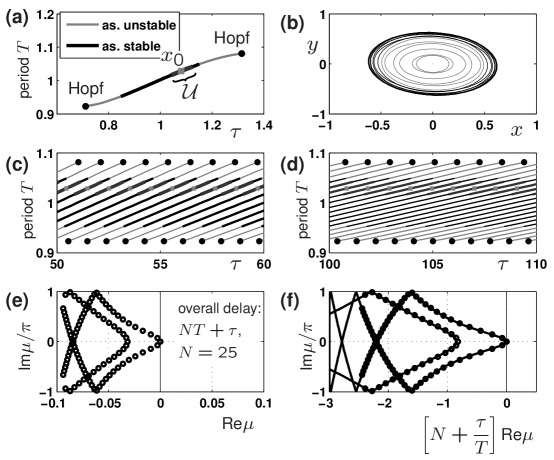
Figure 1. Illustration of stability for the example (2)–(3) (computed with DDE-Biftool [1, 7, 8]): (a) bifurcation diagram of periodic orbits in the $(\tau,T)$-plane; (b) phase portraits of periodic orbits along branch; (c,d) images of the branch under transformation $\tau\mapsto NT(\tau)+\tau$, illustrating overlaps and coexistence; (e) dominant Floquet exponents of selected periodic orbit (grey square in panel (a)); (f) dominant Floquet exponents after rescaling of real parts and curves of asymptotic continuous spectrum. Parameters: $\alpha=-0.10779$ for (a–d), $\tau=1.081$, $N=25$ for (c,d).

Numerically, one can observe that the system has a family of periodic orbits for delays between $\tau\approx 0.7$ and $\tau\approx 1.3$. The period and the phase portrait projected onto the $(x,y)$-plane of these orbits are shown in Figure 1(a) and (b). The family repeats, the orbits keeping their shape, for every integer $N$ if we change the horizontal axis in Figure 1(a) to $NT(\tau)+\tau$. The transformation $NT(\tau)+\tau$ is not just a parallel shift, since the dependence $T(\tau)$ is, generically, nontrivial (in the example $\mathop{}\!\mathrm{d}T/\mathop{}\!\mathrm{d}\tau>0$). This leads to an overlapping of the families for large $\tau$ as shown in Figure 1(c) and (d).

Specifically, let us consider a regular periodic orbit $x_{0}$, existing for a fixed value $\tau_{0}$ of $\tau$ (regularity means that the unit Floquet multiplier of $x_{0}$ is simple, see Section 2). Then $x_{0}$ persists for $\tau$ in a small neighborhood of $\tau_{0}$ such that we have a branch of periodic orbits depending locally on the parameter $\tau$ close to $\tau_{0}$. Let $\mathcal{U}$ be a small neighborhood of this orbit along the branch. Along this branch the period $T$ of the orbit is a smooth function $T(\tau)$ of $\tau$. In Figure 1(a) an example orbit $x_{0}$ is indicated by a grey square at $\tau_{0}=1.081$ and its neighborhood $\mathcal{U}$ is highlighted by a slight thickening of the line. If we assume that $T^{\prime}(\tau_{0})\neq 0$ (which is a genericity condition) then $T(\tau)$ will have a slope uniformly bounded away from zero for all $\tau$ in the neighborhood corresponding to $\mathcal{U}$. This implies that the images of the neighborhood $\mathcal{U}$ are stretched proportionally to $N$ under the transformation $\tau\mapsto NT(\tau)+\tau$. Thus, for any given large $\tau$ a large number of periodic orbits from $\mathcal{U}$ coexist, and the number of coexisting orbits is proportional to $\tau$ (see the overlapping images of $\mathcal{U}$ in Figure 1(c) and (d)).

The next question to ask is: which of those many coexisting periodic orbits for large delays are dynamically stable? Is it possible to derive sharp stability criteria for the large-delay orbits based on quantities independent of the delay? More precisely, what is the stability of a given periodic orbit $x_{0}$ (such as the one indicated by a grey square in Figure 1(a) for delays $\tau=NT(\tau_{0})+\tau_{0}$ as $N$ goes to infinity (this would be the sequence of orbits indicated by grey squares in Figure 1(c,d)).

Our example suggests that the stability for $\tau=NT(\tau_{0})+\tau_{0}$ where $N\to\infty$ can indeed be determined from spectral properties of the periodic orbit at the small delay $\tau_{0}$. Figure 1(e) shows the spectrum of the periodic orbit $x_{0}$ highlighted by a grey square in Figure 1(a) for $N=25$. One can see that, first, its Floquet exponents form bands, and, second, there is a large number of Floquet exponents very close to the imaginary axis (note the scale of the horizontal axis in Figure 1(e)). Figure 1(f) illustrates one of the results of this paper: after rescaling the real part, Floquet exponents converge to curves for $N\to\infty$. These curves, the asymptotic continuous spectrum are computable by solving regular periodic boundary value problems parametrized by $\omega$, the vertical axis in Figure 1(f). Since the original nonlinear DDE is autonomous, one of the curves of the asymptotic continuous spectrum touches the imaginary axis. Similar to the equilibrium case, we establish that the asymptotic continuous spectrum (together with the strongly unstable spectrum, see Section 2) determines the stability of the periodic orbit $x_{0}$ for sufficiently large $N$.

We have colored the branch in Figure 1(a) already according to the conclusions from the asymptotic spectra. The part that is displayed as a black curve in Figure 1(a) is the part of the branch that will be exponentially stable as $N$ tends to infinity, whereas the grey part will be exponentially unstable, having a large number of weakly unstable Floquet exponents.

In short, the observation by Yanchuk & Perlikowski [16] implies that, if we find a periodic orbit $x_{0}$ of the DDE (1) for a fixed small delay $\tau_{0}$, then (under some genericity conditions) the DDE (1) has a large number of similar orbits coexisiting for any sufficiently large delay $\tau$. This paper establishes a sharp critierion (again under some genericity conditions) determining if all of these coexisting periodic orbits are dynamically stable. It does so by providing formulas for the Floquet exponents of the periodic orbit with delay $\tau=NT(\tau_{0})+\tau_{0}$ that are independent of $N$ but valid asymptotically for large $N$. For the example DDE (2)–(3), our results imply that the system has a large number of coexisting stable periodic orbits for every sufficiently large delay $\tau$ (as suggested by the Figures 1(c,d) where the black parts of the branches are stable).

Section 2 gives a non-technical overview of the results gradually developed and proven in the later sections. One central part of our paper is the construction of a characteristic function

$$\mu\mapsto h\left(\mu,\exp(-(NT(\tau_{0})+\tau_{0})\mu)\right)\mbox{,}$$

the roots of which are the Floquet exponents of the periodic orbit for delay $\tau_{0}+NT(\tau_{0})$, and for which we can study the limit $N\to\infty$. This construction is given in Section 3. The existence of this function $h$ permits us to follow the approach from [5] and to extend their techniques to the case of periodic solutions. In the following sections 4 and 5 we describe two parts of the Floquet spectrum that show a different scaling behavior for large $N$ (and, thus, $\tau$). The strongly unstable spectrum, converging to a finite number of asymptotic Floquet exponents which are determined by the instantaneous terms, is investigated in Section 4. Then, in Section 5, we analyze the Floquet exponents given by the asymptotic continuous spectrum shown in Fig 1(f). Based on these results, we can then prove in Section 6 our main result, a criterion about asymptotic stability based on the location of the asymptotic continuous and strongly unstable spectrum.

In contrast to the case of spectra at equilibria, where the asymptotic continuous and strongly unstable spectrum in many cases can be calculated explicitly (see [5]), the corresponding parts of the Floquet spectrum of a periodic orbit $x_{0}$, can typically only be computed numerically. This limitation is not specific to our results but applies equally to most stability results based on the Floquet spectrum for ODEs. Even the periodic orbit itself is in most cases only computable with numerical methods. An exception is the case, where the periodic orbit is at the same time a symmetry orbit of the system. In this case, examples of asymptotic continuous and strongly unstable Floquet spectrum have been calculated explicitly in [15, 17].

Conversely, the results presented in this paper provide an approach to approximate Floquet spectra numerically for large delays $\tau$. If one uses numerical methods on problems with large delays, one faces the difficulty that the size of the matrix arising in the discretized eigenvalue problem grows not only with the desired accuracy (which is natural) but also with $\tau$, even if the period of the orbit remains bounded. This is the case for the numerical methods used in DDE-Biftool [7]. This increase is to be expected because the number of Floquet exponents close to the imaginary axis increases with $\tau$ (see Theorem 6). In contrast to this, the asymptotic spectra can be computed with the same numerical method as in DDE-Biftool and a matrix size that is uniformly bounded for large $\tau$. This paper does not discuss the details of the numerical computation of asymptotic spectra. However, our construction of the characteristic function $h$ is uniform with respect to $\tau$ and could in principle be implemented numerically. In practice, it is better to apply the same analysis as is done in this paper to the large discretized eigenvalue problem.

In Fig. 1(f) we demonstrated the good agreement between original Floquet exponents and asymptotic spectra already in the situation of a moderately large delay, where the original Floquet exponents are still computable. Moreover, our stability criterion, which can be reliably verfied in this way, is valid independently on the actual value of the large delay.

2. Basic concepts and overview of the results

2.1. Periodic orbits, stability, and Floquet exponents

Let $x_{*}$ be a periodic orbit of the $n$-dimensional autonomous nonlinear delay differential equation (DDE)

$$\dot{x}(t)=f(x(t),x(t-\tau))\mbox{,}$$ (4)

that is, $x_{*}(t)$ satisfies (4) for all times $t$ and has period $T$: $x_{*}(t)=x_{*}(t+T)$ for all $t\in\mathbb{R}$. Without loss of generality we may assume that $T=1$ (this can be achieved by a rescaling of time and the delay $\tau$). If the period $T$ is equal to $1$ then $x_{*}$ is also a periodic orbit of

$$\dot{x}(t)=f(x(t),x(t-\tau-N))\mbox{,}$$ (5)

where $N$ is a natural number and $\tau\in[0,1)$. We denote the restriction of the periodic function $x_{*}:\mathbb{R}\mapsto\mathbb{R}^{n}$ to the interval $[-\tau-N,0]$ also by $x_{*}$ such that $x_{*}$ is an element of $C([-\tau-N,0];\mathbb{R}^{n})$.

We are concerned with the question whether the periodic orbit $x_{*}$ is stable or unstable for sufficiently large $N$ in the following sense:

Definition 1 (Exponential orbital stability and instability).

Let $X(t;\cdot)$ be the semiflow on $C([-\tau-N,0];\mathbb{R}^{n})$ induced by DDE (5). The periodic orbit $x_{*}$ is called exponentially orbitally stable if there exists a decay rate $\gamma>0$ such that all initial history segments $x_{0}$ in a neighborhood of $x_{*}$ satisfy

$$\|X(t;x_{0})-X(t+t_{0};x_{*})\|_{\infty}\leq C\exp(-\gamma t)\|x_{0}-x_{*}\|_{\infty}$$

for some time shift $t_{0}$ and some constant $C\geq 0$.

Similarly, $x_{*}$ is called exponentially unstable if there exists a growth rate $\gamma>0$, a neighborhood $\mathcal{N}$ of $x_{*}$ and a constant $C>0$ such that one can find initial history segments $x_{0}\neq x_{*}$ arbitrarily close to $x_{*}$ that satisfy

$$\|X(n;x_{0})-X(n;x_{*})\|_{\infty}\geq C\exp(\gamma n)\|x_{0}-x_{*}\|_{\infty}>0$$

for all $n\in\mathbb{N}$ as long as $X(n;x_{0})$ stays in the neighborhood $\mathcal{N}$.

This is the standard definition for stability of periodic orbits used also for ODEs except that the phase space is $C([-\tau-N,0];\mathbb{R}^{n})$ instead of $\mathbb{R}^{n}$. The notation $\|\cdot\|_{\infty}$ refers to the usual maximum norm in $C([-\tau-N,0];\mathbb{R}^{n})$.

Textbook theory of delay equations reduces the stability problem to the problem of finding eigenvalues of the linear map $M_{N}:C([-\tau-N,0];\mathbb{C}^{n})\to C([-\tau-N,0];\mathbb{C}^{n})$, which is given as the time-$1$ map of the linear DDE

$$\dot{x}(t)=A(t)x(t)+B(t)x(t-\tau-N)\mbox{,}$$ (6)

where the time-dependent $n\times n$-matrices $A(t)\in\mathbb{R}^{n\times n}$ and $B(t)\in\mathbb{R}^{n\times n}$ are the partial derivatives of $f$ in $x_{*}$: $A(t)=\partial_{1}f(x_{*}(t),x_{*}(t-\tau))$ and $B(t)=\partial_{2}f(x_{*}(t),x_{*}(t-\tau))$ [2]. If the right-hand side $f$ of the nonlinear problem (4) is smooth in its arguments then the matrices $A$ and $B$ are also smooth periodic function of time $t$ in the interval $[0,1]$.

Since the time-$1$ map $(M_{N})^{N+1}$ is compact the spectral theory for compact operators and the polynomial spectral mapping theorem imply that the spectrum $\sigma(M_{N})$ consists of a sequence of eigenvalues of finite multiplicity accumulating only at zero (zero is the only element of $\sigma(M_{N})$ that is not in the point spectrum). Also, $\lambda=1$ is always an eigenvalue of $M_{N}$ because $\dot{x}_{*}(t)$ satisfies (6) and has period $1$.

The periodic orbit $x_{*}$ is exponentially (orbitally) stable if and only if

• the eigenvalue $1$ of $M_{N}$ is algebraically simple, and

• all other eigenvalues of $M_{N}$ have modulus less than $1$.

Similarly, it is exponentially unstable if at least one eigenvalue has modulus greater than $1$.

Thus, the stability of iterations of $M_{N}$ is determined by its eigenvalues. We also use the term orbitally stable for the map $M_{N}$, meaning that $M_{N}$ satisfies both of the above conditions.

The state space of DDE (6) is the function space $C([-\tau-N,0];\mathbb{R}^{n})$. Thus, initial value problems for (6) require specifying an infinite-dimensional initial condition. Similarly, one expects that a boundary value problem for a DDE requires the specification of infinitely many boundary conditions. However, periodic boundary value problems are easier to formulate: for example, a solution of the periodic boundary value problem for the general DDE (4) for period $T=1$ is simply a function $x\in C^{1}([-1,0];\mathbb{R}^{n})$ satisfying

$$\dot{x}(t) =f(x(t),x(t-\tau)_{\mathrm{mod}[-1,0]})$$ (7)

$$x(-1) =x(0)$$ (8)

where the notation $(t-\tau)_{\mathrm{mod}[-1,0]}$ stands for $t-\tau+k$ if $t-\tau\in[-k-1,-k)$ and $k\in\mathbb{Z}$ is the integer part of $\tau-t$. Since $x$ is continuous and satisfies the periodicity condition (8) it can be extended continuously to a continuous function on the whole real line by defining $x(s)=x(s_{\mathrm{mod}[-1,0]})$. Consequently, the right-hand side of (7) is continuous for all $t\in[-1,0]$, which guarantees that $x$ can really satisfy the differential equation pointwise and is an element of $C^{1}$. The solution $x$ then automatically satisfies $\dot{x}(-1)=\dot{x}(0)$, and, thus, by induction is as smooth as the right-hand side $f$. In this respect, periodic boundary value problems for DDEs are similar to boundary value problems for ODEs. In Section 3 we will reduce linear periodic boundary value problems for DDEs to low-dimensional linear systems of algebraic equations.

Definition 2.

We call $\mu$ a Floquet exponent of $M_{N}$, and write $\mu\in\Sigma_{N}$, if $\exp(\mu)$ is an eigenvalue of $M_{N}$.

Floquet exponents of $M_{N}$ can be found as those complex numbers $\mu$ for which the periodic boundary value problem

$$\dot{y}(t) =[A(t)-\mu I]y(t)+\exp(-(N+\tau)\mu)\,B(t)\,y((t-\tau)_{\mathrm{mod}[-1,0]})$$ (9)

$$y(0) =y(-1)$$ (10)

has a nontrivial solution $y\in C^{1}([-1,0],\mathbb{C}^{n})$ [2]. Note that in (9) we use the delay $\tau\in[0,1)$ to calculate the Floquet exponents of $M_{N}$, i.e. for a periodic orbit of system (6) with delay $\tau+N$. Only the factor $\exp(-N\mu)$ in front of $B(t)$ accounts for the large delay whereas we have just extended $y$ periodically for arguments less than $-1$. If (9) has a non-trivial solution $y(t)$ for $\mu\in\mathbb{C}$ then it has the non-trivial solution $y(t)\exp(2\pi\mathrm{i}kt)$ for $\mu+2k\pi\mathrm{i}$ for any integer $k$. Hence, we choose the Floquet exponent $\mu$ such that its imaginary part is between $[-\pi,\pi)$.

2.2. Asymptotic spectra for $N\to\infty$

The set of Floquet exponents, $\Sigma_{N}$, forms a discrete subset of the complex plane, the point spectrum of exponents, which depends on $N$. In order to describe in which form $\Sigma_{N}$ has a limit for $N\to\infty$ we introduce two asymptotic spectra, which are also subsets of the complex plane. The notation follows [16].

Definition 3 (Instantaneous and strongly unstable spectrum).

The set $\Sigma_{A}$ of all $\mu\in\mathbb{C}$ for which the linear ODE boundary value problem on $[-1,0]$

$$\dot{y} =[A(t)-\mu I]y$$ (11)

$$y(0) =y(-1)$$ (12)

has a non-trivial solution $y\in C^{1}([-1,0];\mathbb{C}^{n})$ is called the instantaneous spectrum. The subset $\mathcal{A}_{+}\subseteq\Sigma_{A}$ of those $\mu$ with positive real part is called the strongly unstable asymptotic spectrum.

The instantaneous spectrum $\Sigma_{A}$ contains exactly $n$ elements with imaginary part in $[-\pi,\pi)$, counting algebraic multiplicity. We note that $\Sigma_{A}$ and $\mathcal{A}_{+}$ do not depend on $N$ but only on $A$. One result of our paper is that all Floquet exponents of $M_{N}$ with a real part that is positive uniformly in $N$ converge to elements of the strongly unstable spectrum $\mathcal{A}_{+}$.

Yanchuk & Perlikowski [16] observed that the presence of strongly unstable spectrum is not the only possible cause of instability for large $N$. They observed that large numbers of Floquet exponents form bands that have a distance of order $1/N$ from the imaginary axis and have a spacing of order $1/N$ along the imaginary axis. In the limit $N\to\infty$ these bands form curves after a rescaling of the real part by $N$. The limiting curves, called asymptotic continuous spectrum in [16], were defined with the help of a parametric periodic boundary value problem:

Definition 4 (Asymptotic continuous spectrum).

The complex number $\gamma+i\omega\in\mathbb{C}$ ($\gamma\in\mathbb{R}$, $\omega\in[-\pi,\pi)$) lies in the asymptotic continuous spectrum, $\mathcal{A}_{c}$, if the boundary value problem on $[-1,0]$

$$\dot{y}(t) =[A(t)-i\omega I]y(t)+\exp(-\gamma-i\varphi)B(t)y((t-\tau)_{\mathrm{mod}[-1,0]})$$ (13)

$$y(0) =y(-1)$$ (14)

has a non-trivial solution $y\in C^{1}([-1,0]\;R^{n})$ for some $\varphi\in\mathbb{R}$. The quantity $\varphi$ is called the phase corresponding to $\gamma+i\omega$.

Again, the asymptotic continuous spectrum does not depend on $N$ but only on $A$, $B$ and $\tau$.

2.3. A characteristic function for Floquet exponents

We will reduce now the study of the various spectra and their relations to each other to a root-finding problem of a holomorphic function. The following lemma states the existence of a characteristic function for Floquet exponents that at the same time can be used to describe the asymptotic spectra $\mathcal{A}_{+}$ and $\mathcal{A}_{c}$.

Lemma 5 (Characteristic function).

There exists a function $h:\Omega_{1}\times\Omega_{2}\subseteq\mathbb{C}\times\mathbb{C}\mapsto\mathbb{C}$ which is holomorphic in both arguments with the following properties:

1. $\mu$ is a Floquet exponent of $M_{N}$ , i.e. $\mu\in\Sigma_{N}$, if and only if

   $$h(\mu,\exp(-(N+\tau)\mu)=0\mbox{,}$$ (15)

2. $\mu$ is in the instantaneous spectrum $\Sigma_{A}$ if and only if

   $$h(\mu,0)=0\mbox{,}$$ (16)

   and, hence, $\mu$ is in the strongly unstable asymptotic spectrum $\mathcal{A}_{+}$ if

   $$h(\mu,0)=0\mbox{\quad and\quad}\operatorname{Re}\mu>0\mbox{,}$$

3. $\mu=\gamma+i\omega$ is in the asymptotic continuous spectrum $\mathcal{A}_{c}$ if, for some phase $\varphi\in\mathbb{R}$,

   $$h(i\omega,\exp(-\gamma-i\varphi))=0\mbox{.}$$

The algebraic multiplicity of $\mu$ as a Floquet exponent in the statements 1 and 2 equals its multiplicity as a root in (15) and (16).

From property 3 the motivation behind the name asymptotic continuous spectrum becomes clear: if we have a value $\gamma_{0}+i\omega_{0}\in\mathcal{A}_{c}$ and the corresponding phase $\varphi_{0}$, and $\partial_{2}h(i\omega_{0},\exp(-\gamma_{0}-i\varphi_{0}))$ is non-zero (which is generically the case) then a whole curve $\gamma(\omega)+i\varphi(\omega)$ satisfies $h(i\omega,\exp(-\gamma(\omega)-i\varphi(\omega)))=0$ for $\omega\approx\omega_{0}$. These curves are the bands of the asymptotic continuous spectrum. Note that from the existence of the trivial Floquet exponent $\mu=0$ we can conclude that $h(0,1)=0$, which in turn implies that $\gamma=\omega=0$ with phase $\varphi=0$ is in $\mathcal{A}_{c}$. In the generic case where the trivial exponent is contained in a single curve we call it the critical branch of $\mathcal{A}_{c}$.

The details of the construction of $h$, which modifies the general characteristic matrices and functions for periodic delay equations from [10, 13], will be given in section 3. The general characteristic function constructed by [10, 13] may have poles in the complex plane. The modification in Section 3 ensures that these poles of $h(\mu,z)$ stay in the left half-plane. Hence, the domain $\Omega_{1}\times\Omega_{2}$ of $h$ contains all $\mu$ and $z$ satisfying $\operatorname{Re}\mu>-R$ and $|z|<\exp(R)$ where $R>0$ is arbitrary but has to be chosen a-priori. Accordingly, statements 1–3 of Lemma 5 are valid only if both arguments of $h$ satisfy their respective restriction. However, this is the case in the region of interest for stability and bifurcations.

The introduction of the characteristic function $h$ clarifies how the different spectra can be calculated and reduces the analysis of the spectra to a root-finding problem. After defining $h$ properly one could even use $h$ to define the corresponding spectra by the properties listed in Lemma 5.

2.4. Main results

With the help of the asymptotic spectra $\mathcal{A}_{+}$ and $\mathcal{A}_{c}$ we can formulate now a sharp criterion for the exponential orbital stability and instability of $M_{N}$, which is our main result:

Theorem 6 (Stability/Instability).

The map $M_{N}$ (and, hence, the periodic orbit $x_{*}$) is exponentially orbitally stable for all sufficiently large $N$ if all of the following conditions hold:

1. (No strong instability) all elements of the instantaneous spectrum $\Sigma_{A}$ have negative real part (this implies in particular that the strongly unstable spectrum $\mathcal{A}_{+}$ is empty), and

2. (Non-degeneracy) $\partial_{2}h(0,1)\neq 0$, that is, the Floquet exponent $0$ is simple for sufficiently large $N$, and

3. (Weak stability) except for the point $\mu=0$ with phase $\varphi=0$ the asymptotic continuous spectrum $\mathcal{A}_{c}$ is contained in $\{z\in\mathbb{C}:\operatorname{Re}z<0\}$.

The map $M_{N}$ is exponentially unstable for all sufficiently large $N$ if one of the following conditions holds

1. (Strong instability) the strongly unstable spectrum is non-empty, or

2. (Weak instability) a non-empty subset of the asymptotic continuous spectrum $\mathcal{A}_{c}$ has positive real part.

The weak stability condition S-3 is equivalent to stating that for all $\omega\in[-\pi,\pi)$ the function $z\mapsto h(i\omega,\exp(-z))$ has no roots with non-negative real part (with the exception of $z=0$ for $\omega=0$). Similarly, the weak instability condition U-2 is equivalent to stating that $h(i\omega,\exp(-z))=0$ for some $\omega\in[-\pi,\pi)$ and some $z\in\mathbb{C}$ with positive real part.

Several additional corollaries follow from our analysis:

Decay rate and dominant frequency

If $M_{N}$ satisfies S-1–S-3 and is, thus, exponentially stable for all sufficiently large $N$ then the decay rate is at most (and generically) of order $O(N^{-3})$ and the dominant relative frequency is of order $O(N^{-1})$. That is, the dominant non-trivial Floquet exponents are a complex pair of the form $[-CN^{-3}+O(N^{-4})]\pm\mathrm{i}[2\pi/(N+\tau)+O(N^{-2})]$. One branch of the asymptotic continuous spectrum touches the imaginary axis in a (generically quadratic) even-order tangency at $0$, and the dominant non-trivial Floquet exponent lies on this branch and next to the tangency.

Robustness

A map $M_{N}$ that satisfies S-1–S-3 and is, thus, exponentially stable for sufficiently large $N$ according to Theorem 6 remains exponentially stable for all sufficiently large $N$ under all perturbations to $A$, $B$ and $\tau$ of size less than some $\epsilon>0$. This $\epsilon$ does not depend on $N$ because the quantities determining the exponential stability do not depend on $N$ but only on $A$, $B$ and $\tau$. This means that periodic orbits that are stable for large $N$ are uniformly robust with respect to perturbations of the system despite their weak attraction rate of order $N^{-3}$.

This permits the conclusion about the coexistence of stable periodic orbits in the example in Figure 1. The asymptotic spectra of orbits in the small neighborhood $\mathcal{U}$ are small perturbations of the asymptotic spectrum shown in Figure 1(f). In particular the curve touching the imaginary axis will also be curved to the left for all periodic orbits in $\mathcal{U}$.

Spectral approximation

Let the instantaneous spectrum $\Sigma_{A}$ have a positive distance to the imaginary axis. Then we can guarantee that certain points $z$ in the complex plane are in the resolvent set of $M_{N}$ (that is, the periodic boundary value problem (9)–(10) has only the trivial solution for $\mu=z$):

• every point $z$ in the positive half-plane that is not in the strongly unstable spectrum $\mathcal{A}_{+}$ is in the resolvent set of $M_{N}$ for sufficiently large $N$.

• All points of the form $\gamma/(N+\tau)+i\omega$ are in the resolvent set of $M_{N}$ for sufficiently large $N$ if the point $z=\gamma+i\omega$ is not in the asymptotic continuous spectrum $\mathcal{A}_{c}$.

These two statements about the resolvent set of $M_{N}$ imply that the spectrum of $M_{N}$ must be close to $\mathcal{A}_{+}$ or (after rescaling) close to $\mathcal{A}_{c}$. The other direction also holds if the instantaneous spectrum $\Sigma_{A}$ is not on the imaginary axis:

• if $\mu\in\mathcal{A}_{+}$ has multiplicity $k$ then $k$ Floquet exponents of $M_{N}$ converge to $\mu$ for $N\to\infty$ (counting multiplicity).

• Let $\gamma_{*}+i\omega_{*}$ be in the asymptotic continuous spectrum $\mathcal{A}_{c}$, that is,

  $$h(i\omega_{*},\exp(-\gamma_{*}-i\varphi_{*}))=0$$

  for some phase $\varphi_{*}\in[-\pi,\pi)$. Then we will find Floquet exponents $\mu_{N}$ of $M_{N}$ that satisfy (note that this is small-$o$)

  $$\operatorname{Re}\mu_{N}-\frac{\gamma_{*}}{N+\tau}=o(N^{-1})\mbox{,\quad}\operatorname{Im}\mu_{N}-\omega_{*}=o(1)\mbox{.}$$ (17)

  Estimate (17) is rather weak. We need and prove a stronger and more detailed estimate under the additional condition that $\partial_{2}h(i\omega_{*},\exp(-\gamma_{*}-i\varphi_{*}))\neq 0$. Then we have a local root curve $\tilde{\gamma}(\omega)+i\tilde{\varphi}(\omega)$ satisfying $h(i\omega,\exp(-\tilde{\gamma}(\omega)-i\tilde{\varphi}(\omega)))=0$ for $\omega$ near $\omega_{*}$, and for sufficiently large $N$ we find algebraically simple Floquet exponents $\mu_{k}$ of $M_{N}$ satisfying

  $$\operatorname{Im}\mu_{k} =\frac{2k\pi}{N+\tau}+\frac{1}{N+\tau}\tilde{\varphi}\left(\frac{2k\pi}{N+\tau}\right)+O\left((N+\tau)^{-2}\right)$$ (18)

  $$\operatorname{Re}\mu_{k} =\left[1+O\left((N+\tau)^{-1}\right)\right]\frac{\tilde{\gamma}(\operatorname{Im}\mu_{k})}{N+\tau}\mbox{,}$$ (19)

  where $k$ are integers such that $2k\pi/(N+\tau)$ is near $\omega_{*}$, and the $O$-s are smooth functions of $\omega$. These Floquet exponents $\mu_{k}$ form a band of discrete complex numbers approximating the curve $\tilde{\gamma}(\omega)+i\tilde{\varphi}(\omega)$ of asymptotic continuous spectrum.

Degeneracies

Theorem 6 is sharp except for several degenerate cases that are excluded by the conditions S-1–S-3 and U-1–U-2. Degeneracies limiting the region of stable periodic orbits are:

• An element of the instantaneous spectrum $\Sigma_{A}$ has zero real part.

• The partial derivative $\partial_{2}h(0,1)$ equals $0$. In this case the periodic orbit cannot be exponentially stable.

• (Turing and long wavelength instability) The asymptotically continuous spectrum $\mathcal{A}_{c}$ touches the imaginary axis in a quadratic tangency at some value $\pm i\omega_{0}$. In this case the orbit is not exponentially unstable and it is still possible that the periodic orbit is exponentially stable for all $N$ (this is different from the stationary case discussed in [5]) but it may also be weakly stable or unstable. A special case is that $\mathcal{A}_{c}$ touches the imaginary axis in a quadratic tangency in the point $\mu=0$ with phase $\varphi=\pi$. In this case the periodic orbit is still exponentially stable for large $N$.

• (Modulational instability) The critical branch of the asymptotic continuous spectrum $\mathcal{A}_{c}$, containing the trivial exponent $\mu=0$, has a tangency with the imaginary axis at $\omega=0$ that is of higher order than quadratic. In this case the periodic orbit is still exponentially stable according to Theorem 6.

The characteristic function $h$ constructed in Section 3 is still valid for the degenerate cases. However, for a detailed discussion of these degeneracies, one needs not only to specify a defining equation for each degeneracy (this is straightforward) but one also has to state secondary non-degeneracy conditions. In particular the case of instantaneous spectrum with zero real part is somewhat subtle, even though it looks similar to the other listed degeneracies of co-dimension 1 at first sight. In the analogous situation for the spectrum of equilibria, it turns out that instantaneous spectrum $i\omega_{0}$ with zero real part generically implies a singularity of the asymptotic continuous spectrum, $\gamma(\omega_{0})=\infty$, and hence is not part of the stability boundary. Due to these reasons, we believe that a comprehensive treatment of the degeneracies is beyond the scope of the present paper.

3. Construction of the characteristic matrix and function

Let us choose a constant $R>0$ arbitrarily large. We construct a function $h_{N}(\mu)$ that is analytic for all $\mu$ satisfying $\operatorname{Re}\mu\geq-R/(N+\tau)$, and that satisfies $h_{N}(\mu)=0$ if and only if $\mu$ is a Floquet exponent of the map $M_{N}$. Hence, this function can be used to find all Floquet exponents $\mu$ of $M_{N}$ that satisfy $\operatorname{Re}\mu\geq-R/(N+\tau)$. Since we are interested in the stability of the origin under iterates of $M_{N}$, finding the roots of $h_{N}$ will then be sufficient.

We introduce the complex variable $z\in\mathbb{C}$ and consider the periodic boundary value problem for $t\in[-1,0]$

$$\dot{y}(t) =[A(t)-\mu I]y(t)+z\,B(t)\,y((t-\tau)_{\mathrm{mod}[-1,0]}),$$ (20)

$$y(0) =y(-1).$$ (21)

In a first step we will construct a characteristic matrix $\Delta(\mu,z)$ for (20)–(21) such that the roots of its determinant $h(\mu,z)=\det\Delta(\mu,z)$ will be precisely those pairs of points $(\mu,z)$ in some subdomain of $\mathbb{C}\times\mathbb{C}$ for which (20)–(21) has a nontrivial continuously differentiable solution $y\in C^{1}([-1,0];\mathbb{C}^{n})$. Thus, by inserting $z=\exp(-(N+\tau)\mu)$ we will then obtain the characteristic function $h_{N}(\mu)$ in a subdomain of $\mathbb{C}$.

Consider a partition of the periodicity interval $[-1,0]$ into $k$ intervals of size $1/k$:

$$I_{j}=\left[t_{j},t_{j+1}\right)=\left[-1+\frac{j}{k},-1+\frac{j+1}{k}\right)\mbox{\ for $j=0,\ldots,k-1$.}$$ (22)

Using this partition we formulate a multiple initial value problem (MIVP) for a vector of $k$ initial (or restart) values $(v_{0},\ldots,v_{k-1})^{T}\in\mathbb{C}^{nk}$ (similar to multiple shooting):

$$\dot{y}(t) =[A(t)-\mu I]y(t)+zB(t)y((t-\tau)_{\mathrm{mod}[-1,0]})$$ (23)

$$y(t_{i}) =v_{i}\quad\mbox{for $i=0,\ldots,k-1$}$$ (24)

where $t\in[-1,0]$ and $z\in\mathbb{C}$. Notice that in (23) the solution $y$ on the interval $[t_{j},t_{j+1})$ depends on the solution $y(t)$ in other intervals due to the term $y(t-\tau)_{\mathrm{mod}[-1,0]}$ in the right-hand side of (23).

The main purpose of this partition is to reduce the length of the integration interval at the cost of increasing the dimension of the system. Indeed, this construction is very similar to the construction in [11], where in the case of rational $\tau$ a reduction to an equivalent system of ODEs could be achieved, and for the case of irrational $\tau$ corresponding rational approximations have been considered. This can be seen by introducing $u_{j}(t):=y(t+t_{j})$, which satisfy the system of equations

$$\dot{u}_{j}(t) =[A(t+t_{j})-\mu I]u_{j}(t)+zB(t+t_{j})u_{m(j)}((t+t_{j}-t_{m(j)}-\tau)_{\mathrm{mod}[-1,0]})$$ (25)

$$u_{j}(0) =v_{j}$$ (26)

with $j=0,\ldots,k-1$. This system can now be considered as an initial value problem on the interval $[0,1/k)$, and for a solution on this smaller interval $[0,1/k)$ each component $u_{j}(t)$ represents the solution $y(t+t_{j})$ in the corresponding subinterval $I_{j}$. Note that instead of the delayed term $u_{j}((t-\tau)_{\mathrm{mod}[-1,0]})$ we have inserted a coupling to another component $u_{m(j)}((t+t_{j}-t_{m(j)}-\tau)_{\mathrm{mod}[-1,0]})$, where the index $m(j)$ is chosen such that the argument $(t_{j}-t_{m(j)}-\tau)_{\mathrm{mod}[-1,0]}$ is in the interval $[0,1/k)$. The initial value problem for the coupled system (25)–(26) is an equivalent formulation of the multiple initial value problem (23)–(24) and, in a similar way as the boundary value problem (20)–(21), contains both delayed and advanced arguments. If $\tau$ is rational then (25)–(26) is a system of ODEs. This was the starting point for the rational approximations in [11]. We take another route by showing directly that the Picard-Lindelöf iteration for (25)–(26) converges, similar to initial-value problems of ODEs. In the sequel, we will clarify this point, using the formulation (23)–(24) which is more convenient for our purposes.

Let us denote by $U(t,s,\mu)\in\mathbb{R}^{n\times n}$ the propagation matrix of the linear ODE defining the instantaneous spectrum, (11). That is,

$$U(t,s,\mu)v =y(t)\mbox{\quad where}$$

$$y(s) =v\mbox{\quad and}$$

$$\dot{y}(r) =[A(r)-\mu I]y(r)\mbox{\quad for all $r\in[s,t]$.}$$

The norm of $U(t,s,\mu)$ can be estimated by

$$\|U(t,s,\mu)\|_{\infty}\leq\exp\left(\left[\|A\|_{\infty}-\operatorname{Re}\mu\right](t-s)\right)\mbox{.}$$ (27)

In (27) we have used the notation $\|A\|_{\infty}=\max_{t\in[-1,0]}\|A(t)\|_{\infty}$. We will use the same notation for $B$. In order to clarify in which sense system (23)–(24) is an initial value problem and what it means for $y$ to be a solution of system (23)–(24) we formulate an integral equation which is equivalent to (23)–(24):

$$y(t) =[S(\mu)v](t)+z\int\limits_{a_{k}(t)}^{t}U(t,s,\mu)B(s)y((s-\tau)_{\mathrm{mod}[-1,0]}){\mathrm{d}}s$$ (28)

$$[S(\mu)v](t) =U(t,t_{j},\mu)v_{j}\mbox{\quad if $t\in I_{j}$, }$$ (29)

$$a_{k}(t) =t_{j}\mbox{\quad if $t\in I_{j}$.}$$ (30)

We note that $S(\mu)v$ and $a_{k}$ are piecewise continuous functions on $[-1,0]$ ($[S(\mu)v](t)\in\mathbb{C}^{n}$ and $a_{k}(t)\in\mathbb{R}$). They are continuous on each sub-interval $I_{j}=[t_{j},t_{j+1})$ but have jumps at the times $t_{j}$. The integral equation (28) is a fixed-point problem for $y$. If we find a fixed point $y$ then $y$ may have discontinuities at the times $t_{j}$. Thus, the appropriate space in which to look for solutions of the fixed point problem (28) is the space of piecewise continuous functions with the usual $\max$-norm $\|y\|_{\infty}$:

$$C_{k}= \begin{aligned} \{&y:[-1,0]\mapsto\mathbb{C}^{n}:\mbox{\ $y$ continuous on each subinterval $I_{j}=[t_{j},t_{j+1})$}\\ &\mbox{\ ($j=0,\ldots,k-1$) and $\lim_{t\nearrow t_{j}}y(t)$ exists for all $j=1\ldots k$.}\}\end{aligned}$$ (31)

The right-hand side of the integral equation (28) is an affine map, mapping $C_{k}$ back to itself such that (28) is of the form

$$y=S(\mu)v+zL_{k}(\mu)y$$ (32)

where $S(\mu):\mathbb{C}^{nk}\mapsto C_{k}$ is defined by (29), and $L_{k}(\mu)y$ is the linear part of the right-hand side in (28) (that is, the integral term). The linear map $L_{k}(\mu):C_{k}\mapsto C_{k}$ is continuously differentiable (and, thus, holomorphic) with respect to the complex variable $\mu$. A simple estimate for the norm of $L_{k}$ with respect to the $\|\cdot\|_{\infty}$-norm gives us the unique solvability of the fixed point problem (32) (which is actually the integral equation (28)–(30)):

Lemma 7 (Existence and Uniqueness of solutions for IVP).

Let $R>0$ be arbitrary. If we set the number of sub-intervals, $k$, such that

$$k>C(R):=\max\left\{\|A\|_{\infty}+R,\|B\|_{\infty}\exp(1+R)\right\}$$ (33)

then the affine integral equation (28)–(30) has a unique solution $y\in C_{k}$ for all $\mu$ and $z$ satisfying

$$\operatorname{Re}\mu\geq-R\mbox{,\qquad}|z|\leq\exp(R)$$ (34)

and all tuples $(v_{0},\ldots,v_{k})^{T}\in\mathbb{C}^{nk}$.

The details of the norm estimate for $L_{k}$ are in Appendix A. The solution $y$ can be written as $y=[I-zL_{k}(\mu)]^{-1}S(\mu)v$. When is this solution $y$ (which is only in $C_{k}$ for general $v$) continuously differentiable on the whole interval? This requirement is a linear condition on the tuple $v$. Let us fix a constant $R>0$ and choose the number of sub-intervals $k>C(R)$.

Definition 8 (Characteristic matrix and function).

We define the characteristic matrix $\Delta(\mu,z)\in\mathbb{C}^{nk\times nk}$ for the problem (23)-(24) as

$$\Delta(\mu,z)v:=\Delta(\mu,z)\begin{bmatrix}v_{0}\\ \vdots\\ v_{k-1}\end{bmatrix}:=\begin{bmatrix}v_{0}-y(0)\\ v_{1}-\lim_{t\nearrow t_{1}}y(t)\\ \vdots\\ v_{k-1}-\lim_{t\nearrow t_{k-1}}y(t)\end{bmatrix}\mbox{.}$$ (35)

and the corresponding characteristic function $h(\mu,z)$ as

$$h(\mu,z):=\det\Delta(\mu,z)\mbox{.}$$ (36)

Note that the integral equation (28) implies that $v_{j}=\lim_{t\searrow t_{j}}y(t)$. In this sense the values $v_{j}$ are the initial (or restart) values for the differential equation (23). The construction of $\Delta$ gives a well-defined matrix for all $z$ and $\mu$ satisfying $\operatorname{Re}\mu\geq-R$ and $|z|\leq\exp(R)$: for a given tuple $v$ we evaluate the unique solution $y=[I-zL_{k}(\mu)]^{-1}S(\mu)v\in C_{k}$ of the integral equation (28) and then we use this $y$ to evaluate the right-hand side of (35). The characteristic matrix $\Delta$ is set up such that for $v$ in the kernel of $\Delta(\mu,z)$ the solution $y$ also satisfies the differential equation (23) on the whole interval (and does not have jumps) including the periodic boundary conditions:

Lemma 9 (Differentiability).

Let $\operatorname{Re}\mu\geq-R$, $|z|\leq\exp(R)$ and $k>C(R)$. If the tuple $v=(v_{0},\ldots,v_{k-1})$ satisfies

$$\Delta(\mu,z)v=0$$ (37)

then $y=[I-zL_{k}(\mu)]^{-1}S(\mu)v$, the solution of the integral equation (28), is continuously differentiable on $[-1,0]$ and satisfies the differential equation (20) with the periodic boundary condition (21). Conversely, let $y\in C^{1}([-1,0],\mathbb{C}^{n})$ be a continuously differentiable solution of (20)–(21). Then the tuple $v=(v_{0},\ldots,v_{k-1})\in\mathbb{C}^{k}$, where $v_{0}=y(-1)$, $v_{1}=y(t_{1})$, $\dots$, $v_{k-1}=y(t_{k-1})$ satisfies (37).

Proof.

The rows $2$ to $k$ of the right-hand side in the definition (35) of $\Delta$ ensure continuity of $y$: since $v_{j}=\lim_{t\searrow t_{j}}y(t)$ for $j=1,\ldots,k-1$ the condition that these rows are equal to zero reads $\lim_{t\searrow t_{j}}y(t)=\lim_{t\nearrow t_{j}}y(t)$, and (by inserting the right-hand side of (28))

$$v_{j+1}=U(t_{j+1},t_{j},\mu)v_{i}+z\int\limits_{t_{j}}^{t_{j+1}}U(t_{j+1},s,\mu)B(s)y((s-\tau)_{\mathrm{mod}[-1,0]}){\mathrm{d}}s$$

for $j=0,\ldots,k-1$. This implies that $y$ is continuous on $[-1,0]$, and that we can concatenate all the integral terms in (28) to

$$y(t)=U(t,-1,\mu)v_{0}+z\int_{-1}^{t}U(t,s,\mu)B(s)y((s-\tau)_{\mathrm{mod}[-1,0]}){\mathrm{d}}s$$ (38)

The first row of the condition $\Delta(\mu,z)v=0$ reads $v_{0}=y(0)$, which makes sure that $y$ is periodic at the boundary of $[-1,0]$, and guarantees that the integrand in (38) is continuous at $s=\tau-1$. Consequently, the integrand is continuous everywhere, which implies that $y$ is continuously differentiable. Thus, we can differentiate (38) with respect to $t$, which implies that $y$ satisfies the differential equation (20). This, in turn, implies that also $\dot{y}(-1)=\dot{y}(0)$ because the right-hand side of (20) is periodic. ∎

Since the map $L_{k}$ depends analytically on $\mu$, the matrix $\Delta$ depends analytically on $\mu$ and $z$, too (as long as $\operatorname{Re}\mu\geq-R$ and $|z|\leq\exp(R)$). Calling $\Delta$ the characteristic matrix makes sense for the following reason:

Lemma 10 (Characteristic function for (6) [10]).

Let $N\geq 1$ and $R>0$ be given, and choose the number of sub-intervals, $k$, greater than $C(R)$. Then for all $\mu$ satisfying

$$\operatorname{Re}\mu\geq-\frac{R}{N+\tau}$$

the following equivalence holds: $\mu$ is a Floquet exponent of the time-$1$ map $M_{N}$ of the periodic linear DDE (6) if and only if

$$h_{N}(\mu):=h(\mu,\exp(-(N+\tau)\mu))=\det\Delta(\mu,\exp(-(N+\tau)\mu))=0\mbox{.}$$ (39)

The algebraic multiplicity of $\mu$ as a Floquet exponent of $M_{N}$ is equal to the order of $\mu$ as a root of $h_{N}$.

Proof.

That $\mu$ is a Floquet exponent of (6) if and only if $\Delta(\mu,\exp(-(N+\tau)\mu))$ has a non-trivial kernel is clear because Floquet exponents of $M_{N}$ were defined as those complex numbers for which (20)–(21) has a non-trivial solution. The statement about the multiplicity of $\mu$ follows from arguments similar to [3], which are laid out in detail in [10] (an equivalence between the eigenvalue problem for $M_{N}$, $\exp(\mu)v-M_{N}v=0$, and the algebraic equation $\Delta(\mu,\exp(-(N+\tau)\mu))v=0$ is constructed in [10]). ∎

Both functions, $h$ and $h_{N}$, are real analytic (that is, their expansion coefficients are real numbers since $A$, $B$ and $\tau$ are real).

For any given $R>0$ we have chosen $k>0$ and constructed a characteristic function $h_{N}(\mu)$, defined on the half plane

$$\left\{\mu\in\mathbb{C}\mid\operatorname{Re}\mu\geq-\frac{R}{N+\tau}\right\}\mbox{,}$$

the roots of which are precisely the Floquet exponents (counting multiplicities) of the period map $M_{N}$ for the linearized delay differential equation (6).

As we are interested in the location of Floquet exponents of the time-$1$ map $M_{N}$ to the right or close to the imaginary axis we have reduced the eigenvalue problem to a study of the asymptotic behavior of roots of the holomorphic function $h_{N}$ for $N\to\infty$. Furthermore, the asymptotic spectra are defined as roots and root curves of $h$ by construction of $h$: $\mu>0$ is in the strongly unstable spectrum $\mathcal{A}_{+}$ if and only if $h(\mu,0)=0$, and $\mu=\gamma+i\omega$ is in the asymptotic continuous spectrum $\mathcal{A}_{c}$ if and only if $h(i\omega,\exp(-\gamma-i\varphi))=0$ for some phase $\varphi\in\mathbb{R}$.

This proves Lemma 5 and allows us to follow an approach similar to [17, 5] in the following sections. Note that in the case where the period and the delay are rationally dependent, the existence of a suitable characteristic function follows much easier (see [11]), but the structure of the asymptotic spectra discussed below will be not affected.

4. Strongly unstable spectrum

One immediate consequence of Lemma 5 is the statement asserted in [16] for the relation between eigenvalues of $M_{N}$ and the strongly unstable spectrum $\mathcal{A}_{+}$. Note that $\mu$ is in the strongly unstable spectrum $\mathcal{A}_{+}$ if and only if $h(\mu,0)=0$: if one sets $z=0$ in (20) the differential equation reduces to (11), the expression defining $\mathcal{A}_{+}$. For large $N$ unstable Floquet exponents of $M_{N}$ either approach the imaginary axis or $\mathcal{A}_{+}$:

Lemma 11 (Convergence to strongly unstable spectrum).

Let $\operatorname{Re}\mu_{0}>0$. If $h(\mu_{0},0)\neq 0$ then there exists a $N_{0}$ such that $\mu_{0}$ lies in the resolvent set of the time-$1$ map $M_{N}$ for all $N>N_{0}$.

If $\mu_{0}$ is a root of multiplicity $k$ of the function $h(\cdot,0)$ then every sufficiently small neighborhood $U$ of $\mu_{0}$ contains exactly $k$ Floquet exponents (counting multiplicity) of $M_{N}$ for all $N>N_{0}$ ($N_{0}$ depends on $U$).

The resolvent set is the set of all complex numbers $\mu$ for which the map $\exp(\mu)I-M_{N}$ is an isomorphism (characterized by $h_{N}(\mu)\neq 0$ for $\operatorname{Re}\mu\geq-R/(N+\tau)$).

Proof.

The statement for $h(\mu_{0},0)\neq 0$ follows from expansion of $h(\mu_{0},\cdot)$ in $z=0$ since $z=\exp(-(N+\tau)\mu_{0})\to 0$ for $N\to\infty$ if $\operatorname{Re}\mu_{0}>0$.

Let $\mu_{0}$ be a root of $h(\cdot,0)$ of multiplicity $k$. For any sufficiently small $\delta>0$, $\mu_{0}$ is the only root of $h(\cdot,0)$ inside the ball $B_{\delta}(\mu_{0})$ of radius $\delta$ around $\mu_{0}$. In particular, $h(\mu,0)\neq 0$ on the boundary of $B_{\delta}(\mu_{0})$. Then $h(\mu,\exp(-(N+\tau)\mu))$ is also non-zero on the boundary of $B_{\delta}(\mu_{0})$ for sufficiently large $N$, and the logarithmic derivative of $h(\mu,\exp(-(N+\tau)\mu))$ converges for $N\to\infty$:

$$\frac{\frac{{\mathrm{d}}}{{\mathrm{d}}\mu}[h(\mu,\exp(-(N+\tau)\mu))]}{h(\mu,\exp(-(N+\tau)\mu))}=$$

$$\frac{\partial_{1}h(\mu,\exp(-(N+\tau)\mu))-(N+\tau)\exp(-(N+\tau)\mu)\partial_{2}h(\mu,\exp(-(N+\tau)\mu))}{h(\mu,\exp(-(N+\tau)\mu))}$$

$$\to_{N\to\infty}\frac{\partial_{1}h(\mu,0)}{h(\mu,0)}\mbox{\quad if $\operatorname{Re}\mu>0$ for all $\mu\in B_{\delta}(\mu_{0})$.}$$

Thus, the line integral of the logarithmic derivative of $h(\mu,\exp(-(N+\tau)\mu))$ along the boundary of $B_{\delta}(\mu_{0})$, which counts the roots (and poles), also converges for $N\to\infty$ to the logarithmic derivative of $h(\cdot,0)$. Since the line integral of the logarithmic derivative is an integer it must be constant for $N\to\infty$, and, hence, $h_{N}(\mu)$ must have the same number of roots (counting multiplicity) inside $B_{\delta}(\mu_{0})$ as $h(\cdot,0)$, which is $k$. ∎

Lemma 11 shows that $M_{N}$ is exponentially unstable for all sufficiently large $N$ if the strongly unstable spectrum is non-empty, which is condition U-1 of Theorem 6.

5. Asymptotic continuous spectrum

Due to Lemma 5 the asymptotic continuous spectrum is given as those $\mu=\gamma+i\omega$ for which one can find a phase $\varphi\in\mathbb{R}$ such that $h(i\omega,\exp(-\gamma-i\varphi))=0$.

Thus, we expect the asymptotic continuous spectrum to come in curves: Let $\gamma_{0}+i\omega_{0}\in\mathcal{A}_{c}$ be a point in the asymptotic continuous spectrum and let $\varphi_{0}\in[-\pi,\pi)$ be its phase. By definition $\mu_{0}=\gamma_{0}+i\varphi_{0}\in\mathbb{C}$ satisfies $0=h(i\omega_{0},\exp(-\mu_{0}))$. If $\partial_{2}h(i\omega_{0},\exp(-\mu_{0}))\neq 0$ then there is a root curve $\mu(\omega)$ of complex numbers satisfying $h(i\omega,\exp(-\mu(\omega)))=0$ going through $\mu_{0}$. Hence locally (for $\omega$ in a neighborhood of $\omega_{0}$) there is a curve $\omega\mapsto(\operatorname{Re}\mu(\omega)+i\omega)\in\mathcal{A}_{c}$ through $\gamma_{0}+i\omega_{0}$ for $\omega$ near $\omega_{0}$ .

We assume for the remainder of the section that the instantaneous spectrum $\Sigma_{A}$ has a positive distance to the imaginary axis. The idea behind the construction of the asymptotic continuous spectrum is that for Floquet exponents $\mu$ close to the imaginary axis, that is, for $\mu$ of the form

$$\mu=\frac{\gamma}{N+\tau}+i\omega$$ (40)

with a bounded factor $\gamma$ in the real part, the roots of the characteristic function $h_{N}(\mu)=h(\mu,\exp(-(N+\tau)\mu))$ converge to a regular limit for $N\to\infty$ after inserting the scaling (40). This can be made more specific: if the instantaneous spectrum $\Sigma_{A}$ has a positive distance from the imaginary axis then all Floquet exponents that are not converging to the strongly unstable spectrum have a real part less than $R_{2}/(N+\tau)$ where $R_{2}$ does not depend on $N$:

Lemma 12 (Convergence to the imaginary axis).

Assume that the elements of the instantaneous spectrum $\Sigma_{A}$ have a positive distance $2\epsilon>0$ from the imaginary axis. Let us denote the points in the strongly unstable spectrum, $\mathcal{A}_{+}$, by $\mu_{1}$,…, $\mu_{j}$. There exists a constant $R_{2}\geq 0$ such that all Floquet exponents $\mu$ of $M_{N}$ satisfy either $\mu\in B_{\epsilon}(\mu_{j})$ for some $j$, or

$$\operatorname{Re}\mu<\frac{R_{2}}{N+\tau}$$ (41)

for all $N\geq 1$.

Proof.

For all complex numbers $\mu$ that have non-negative real part and are outside of the balls $B_{\epsilon}(\mu_{j})$ the matrix $I-U(0,-1,\mu)$ is invertible and the inverse has a uniform upper bound (remember that $U$ is the propagation matrix of $\dot{y}=[A(t)-\mu I]y$):

$$\left\|[I-U(0,-1,\mu)]^{-1}\right\|\leq C\mbox{.}$$

We also know that $\mu$ is a Floquet exponent if the integral equation (38) (which is equivalent to the differential equation (37)) has a non-trivial periodic solution $y(t)$ for $z=\exp(-(N+\tau)\mu)$. This implies ($y(-1)=y(0)=v_{0}$)

$$v_{0}=U(0,-1,\mu)v_{0}+z\int_{-1}^{0}U(0,s,\mu)B(s)y((s-\tau)_{\mathrm{mod}[-1,0]}){\mathrm{d}}s\mbox{,}$$

and, hence,

$$\begin{split}y(t)=&z\left[[I-U(0,-1,\mu)]^{-1}\int_{-1}^{0}U(0,s,\mu)B(s)y((s-\tau)_{\mathrm{mod}[-1,0]}){\mathrm{d}}s+\right.\\ &\phantom{z}+\left.\int_{-1}^{t}U(t,s,\mu)B(s)y((s-\tau)_{\mathrm{mod}[-1,0]}){\mathrm{d}}s\right]\end{split}$$ (42)

The factor of $z$ in the right-hand side of this fixed-point problem for $y$ is a linear operator $K(\mu)$ on the space of continuous functions. $K(\mu)$ is uniformly bounded for all $\mu$ that have non-negative real part and are outside of the balls $B_{\epsilon}(\mu_{j})$. Let us denote an upper bound on the norm of $K(\mu)$ by $C_{1}$. Then for all $z$ satisfying $|z|<C_{1}^{-1}$ the integral equation (38) cannot have a non-trivial solution. Since, for Floquet exponents of $M_{N}$, $z$ equals $\exp(-(N+\tau)\mu)$ this means that $\mu$ has to satisfy

$$|\exp(-(N+\tau)\mu)|\geq C_{1}^{-1}\mbox{,}$$

and, thus

$$\operatorname{Re}\mu\leq\frac{\log C_{1}}{N+\tau}$$

for $|z|$ to be larger than $C_{1}^{-1}$. Consequently, if we choose $R_{2}>\log C_{1}$ then a $\mu$ that has non-negative real part and lies outside of the balls $B_{\epsilon}(\mu_{j})$ must satisfy (41) in order to be a Floquet exponent of $M_{N}$. ∎

A corollary of the construction described by equation (42) is that for each $\omega$ the intersection of the asymptotic continuous spectrum $\mathcal{A}_{c}$ with the horizontal line $\{\mu\in\mathbb{C}:\operatorname{Im}\mu=\omega\}$ can be described as a set of eigenvalues of a compact operator $K(\mathrm{i}\omega)$. Thus, if $\operatorname{Re}\Sigma_{A}\neq 0$ the asymptotic continuous spectrum forms curves parametrizable by $\omega$, which may only have poles at $-\infty$:

Corollary 13 (Asymptotic continuous spectrum consists of curves).

Assume that the instantaneous spectrum $\Sigma_{A}$ has a positive distance to the imaginary axis. A point $\mu$ is in the asymptotic continuous spectrum if $\exp(\mu)$ is an eigenvalue of the compact linear operator $K(\mathrm{i}\omega):C([-1,0];\mathbb{C}^{n})\mapsto C([-1,0];\mathbb{C}^{n})$ given by

$$K(\mathrm{i}\omega)y:= \left[[I-U(0,-1,\mathrm{i}\omega)]^{-1}\int_{-1}^{0}U(0,s,\mathrm{i}\omega)B(s)y((s-\tau)_{\mathrm{mod}[-1,0]}){\mathrm{d}}s+\right.$$

$$\phantom{z}+\left.\int_{-1}^{t}U(t,s,\mathrm{i}\omega)B(s)y((s-\tau)_{\mathrm{mod}[-1,0]}){\mathrm{d}}s\right]\mbox{.}$$

In particular there exists a constant $R_{3}\geq 0$ so that the asymptotic continuous spectrum lies to the left of the vertical line $\{z\in\mathbb{C}:\operatorname{Re}z=R_{3}\}$.

The matrix $U$ in the definition of $K$ is the monodromy matrix of the instantaneous problem $\dot{x}(t)=[A(t)-\mathrm{i}\omega]x(t)$. The inverse of $I-U(0,-1,\mathrm{i}\omega)$ exists because of our assumption that the instantaneous spectrum, $\Sigma_{A}$, does not contain points on the imaginary axis. The corollary implies that the asymptotic continuous spectrum consists of curves even in points where the regularity condition on $\partial_{2}h\neq 0$ is violated. In these points $K(\mathrm{i}\omega)$ has eigenvalues of finite multiplicity larger than $1$ such that finitely many curves of the asymptotic continuous spectrum cross each other (or are on top of each other).

All Floquet exponents of $M_{N}$ that do not converge to the strongly unstable spectrum for $N\to\infty$ (these can be at most $n$, equaling the dimension of $A(t)$) are either stable, or they satisfy restriction (41) on the upper bound. Thus, apart from the strongly unstable spectrum, the multipliers, which are of interest from the point of view of stability and bifurcations, lie in the strip

$$\mathcal{C}_{N}:=\left\{\mu\in\mathbb{C}:-\frac{R}{N+\tau}\leq\operatorname{Re}\mu\leq\frac{R_{2}}{N+\tau}\right\}$$

and have the form

$$\mu=\frac{\gamma}{N+\tau}+\mathrm{i}\omega\mbox{\quad where $\gamma\in[-R,R_{2}]$ and $\omega\in[-\pi,\pi)$}$$ (43)

(after shifting them into the strip $\{z:\operatorname{Im}z\in[-\pi,\pi)\}$ by subtraction of an integer multiple of $2\pi\mathrm{i}$). As we focus our discussion on Floquet exponents of the scale (43) from now on it makes sense to introduce the notation of a scaled Floquet exponent.

Definition 14 (Scaled Floquet exponent & resolvent set).

A complex number $\mu=\gamma+\mathrm{i}\omega$ with $\gamma\in[-R,R_{2}]$ and $\omega\in[-\pi,\pi)$ is called a scaled Floquet exponent of $M_{N}$ if $\gamma/(N+\tau)+\mathrm{i}\omega$ is a Floquet exponent of $M_{N}$. Similarly, $\mu$ is in the scaled resolvent set of $M_{N}$ if $\gamma/(N+\tau)+\mathrm{i}\omega$ is in the resolvent set of $M_{N}$.

We can now formulate precisely in which sense the asymptotic continuous spectrum $\mathcal{A}_{c}$ is the limit of the spectra of $M_{N}$. First, we make a statement about resolvent sets.

Lemma 15 (Points distant from $\mathcal{A}_{c}$).

Let the instantaneous spectrum $\Sigma_{A}$ have a positive distance to the imaginary axis. If $\gamma_{0}>-R$ and $\gamma_{0}+i\omega_{0}$ is not in the asymptotic continuous spectrum $\mathcal{A}_{c}$ then $\gamma_{0}+i\omega_{0}$ is in the scaled resolvent set of $M_{N}$ for sufficiently large $N$.

Proof.

Lemma 15 is a simple consequence of the fact that, if $h(i\omega_{0},\exp(-\gamma_{0}-i\varphi))\neq 0$ for all phases $\varphi\in[-\pi,\pi]$ (which defines points $\gamma_{0}+i\omega_{0}\notin\mathcal{A}_{c}$ if $\gamma_{0}>-R$) then

$$h_{N}\left(\frac{\gamma_{0}}{N+\tau}+i\omega_{0}\right)=h\left(i\omega_{0}+\frac{\gamma_{0}}{N+\tau},\exp\left(-\gamma_{0}-i(N+\tau)\omega_{0}\right)\right)\neq 0$$

for all sufficiently large $N$. Lemma 5 implies that $\gamma_{0}/(N+\tau)+i\omega_{0}$ is in the resolvent set of $M_{N}$ for all sufficiently large $N$. ∎

Lemma 15 implies that all spectrum of $M_{N}$ near the imaginary axis has to be close to $\mathcal{A}_{c}$ even after blow-up of the real part. The other direction, that every point of $\mathcal{A}_{c}$ in the strip $-R<\operatorname{Re}\mu<R_{2}$ is approached by scaled Floquet exponents of $M_{N}$, is also true (again under the assumption that the instantaneous spectrum $\Sigma_{A}$ is not on the imaginary axis). We prove this direction first for regular root curves of $h$ because this is the most common case, and the missing piece for the stability criterion. Our estimate is slightly sharper than mere approximation to make it useful for our proof of the stability criterion.

In short, Lemma 16 below states that any regular curve of asymptotic continuous spectrum, $\tilde{\gamma}(\omega)+\mathrm{i}\omega$ (with its corresponding phase $\tilde{\varphi}(\omega)$), is approximated by scaled Floquet exponents of the form $\gamma_{k}+\mathrm{i}\omega_{k}$ where

$$\omega_{k} =\frac{2k\pi}{N+\tau}+\frac{1}{N+\tau}\tilde{\varphi}\left(\frac{2k\pi}{N+\tau}\right)+O\left((N+\tau)^{-2}\right)$$ (44)

$$\gamma_{k} =\left[1+O\left((N+\tau)^{-1}\right)\right]\tilde{\gamma}(\omega_{k})\mbox{,}$$ (45)

$k$ are integers such that $2k\pi/(N+\tau)$ is near $\omega$, and the $O$-s are smooth functions of $\omega$. This proves the stronger estimate (18)–(19), given in the non-technical overview in Section 2.

Lemma 16 (Convergence to regular curves of $\mathcal{A}_{c}$).

Assume that the triplet $(\omega_{*},\gamma_{*},\varphi_{*})$ satisfies

$$h(\mathrm{i}\omega_{*},\exp(-\gamma_{*}-\mathrm{i}\varphi_{*}))=0\mbox{,\quad}\partial_{2}h(\mathrm{i}\omega_{*},\exp(-\gamma_{*}-\mathrm{i}\varphi_{*}))\neq 0\mbox{.}$$

Let $N_{*}$ be sufficiently large and $\delta>0$ be sufficiently small. We denote the unique regular root curve of $\mu\mapsto h(\mathrm{i}\omega,\exp(-\mu))$ for $\omega$ near $\omega_{*}$ through $(\omega=\omega_{*},\mu_{*}=\gamma_{*}+\mathrm{i}\varphi_{*})$ by

$$\tilde{\mu}(\omega)=\tilde{\gamma}(\omega)+\mathrm{i}\tilde{\varphi}(\omega)\mbox{.}$$

For all $N\geq N_{*}$ there are scaled Floquet exponents $\mu_{N,k}$ of $M_{N}$ near $\gamma_{*}+i\omega_{*}$. All scaled Floquet exponents $\mu_{N,k}$ that are sufficiently close to $\gamma_{*}+i\omega_{*}$ are algebraically simple and have the form

$$\mu_{N,k}=\tilde{\gamma}_{N}(\omega_{k})+i\omega_{k}\mbox{,}$$ (46)

where:

• $k$ is any integer satisfying

  $$\frac{2k\pi}{N+\tau}\in(\omega_{*}-\delta,\omega_{*}+\delta)\mbox{,}$$

• $\omega_{k}$ is the unique solution of the fixed point problem for $\omega$

  $$\omega=\frac{\tilde{\varphi}_{N}(\omega)}{N+\tau}+\frac{2k\pi}{N+\tau}\mbox{,}$$ (47)

• the functions $\tilde{\gamma}_{N}$ and $\tilde{\varphi}_{N}$ are perturbations of $\tilde{\gamma}(\omega)$ and $\tilde{\varphi}(\omega)$ of the form

  $$\tilde{\gamma}_{N}(\omega) =\left[1+\frac{1}{N+\tau}\operatorname{Re}g\left(\omega,\frac{1}{N+\tau}\right)\right]\tilde{\gamma}(\omega)$$ (48)

  $$\tilde{\varphi}_{N}(\omega) =\tilde{\varphi}(\omega)+\frac{1}{N+\tau}\operatorname{Im}g\left(\omega,\frac{1}{N+\tau}\right)\tilde{\gamma}(\omega)$$ (49)

  where $g(\omega,\epsilon)$ is a smooth complex-valued function, which is independent of $N$ and defined for $\omega\in(\omega_{*}-\delta,\omega_{*}+\delta)$ and $\epsilon\in[0,1/N_{*})$.

We notice that the scaled Floquet exponents of $M_{N}$ lie on bands: they are on the curve given by $\tilde{\gamma}_{N}(\omega)+\mathrm{i}\omega$, which is a small perturbation of the curve of asymptotic continuous spectrum $\tilde{\gamma}(\omega)+\mathrm{i}\omega$. The spacing between scaled Floquet exponents along this band is given by the fixed point equation (47). The fixed point problem (47) is only weakly implicit since the right-hand side terms containing $\omega$ all have a pre-factor $1/(N+\tau)$, which is small. Hence, expression (45) for $\gamma_{k}$ follows immediately from (48) and expression (44) for $\omega_{k}$ follows from (47) and (49).

Proof.

(of Lemma 16) We know that $\tilde{\gamma}(\omega)+\mathrm{i}\tilde{\varphi}(\omega)$ is a regular root curve of

$$h(i\omega,\exp(-\gamma-\mathrm{i}\varphi))=0\mbox{.}$$ (50)

The root problem

$$h\left(\mathrm{i}\omega+\epsilon\gamma,\exp\left(-\gamma-\mathrm{i}\varphi\right)\right)=0$$

is for small $\epsilon$ a small (order $\epsilon$) perturbation of the root problem (50). Thus, for sufficiently small $\epsilon$, a root curve of the form $\tilde{\gamma}_{\epsilon}(\omega)+\mathrm{i}\tilde{\varphi}_{\epsilon}(\omega)$ exists for $\omega$ in some neighborhood of $\omega_{*}$, and it has the form

$$\tilde{\gamma}_{\epsilon}(\omega)+\mathrm{i}\tilde{\varphi}_{\epsilon}(\omega)=\left[1+\epsilon g\left(\omega,\epsilon\right)\right]\tilde{\gamma}(\omega)+\mathrm{i}\tilde{\varphi}(\omega)\mbox{,}$$ (51)

where $g(\omega,\epsilon)$ is a smooth complex-valued function defined for $\omega$ in a small neighborhood of $\omega_{*}$ and $\epsilon\in[0,\epsilon_{\max})$ (with some $\epsilon_{\max}>0$). Note that the error term contains a factor $\tilde{\gamma}(\omega)$, making the error equal to zero on the imaginary axis. (See Appendix B for details of how to extract this factor from the error.) Inserting $\epsilon=(N+\tau)^{-1}$ and labeling the curves $\tilde{\gamma}_{\epsilon}(\omega)$ as $\tilde{\gamma}_{N}(\omega)$ and $\tilde{\varphi}_{\epsilon}$ as $\tilde{\varphi}_{N}$ gives the definitions (48) and (49) in the lemma. Correspondingly, we make an initial choice for the minimal $N$, $N_{*}$, as $1/\epsilon_{\max}$.

A point on the curve $\tilde{\gamma}_{N}(\omega)+\mathrm{i}\omega$ is a scaled Floquet exponent of $M_{N}$ if and only if its imaginary part $\omega$ satisfies

$$\exp(-\mathrm{i}\omega(N+\tau)) =\exp(-\mathrm{i}\tilde{\varphi}_{N}(\omega))\mbox{\quad and, thus,}$$

$$(N+\tau)\omega =\tilde{\varphi}_{N}(\omega)+2k\pi\mbox{\quad\ \ for some integer $k\in\mathbb{Z}$.}$$

After dividing by $N+\tau$ this becomes the fixed point equation (47) for $\omega$. For which $k$ does this fixed point problem have a unique solution?

We choose a neighborhood $\mathcal{U}$ of $\omega_{*}$ of the form $(\omega_{*}-2\delta,\omega_{*}+2\delta)$ such that $\tilde{\varphi}_{N}$ is well-defined for all $\omega\in\mathcal{U}$ and all $N\geq N_{*}$, and satisfies $|\tilde{\varphi}_{N}^{\prime}(\omega)|<L$ for some constant $L$ (which is independent of $N$). Next, we increase $N_{*}$ such that

$$\frac{L}{N+\tau} <1\mbox{\quad for all $N>N_{*}$, and}$$

$$\frac{\tilde{\varphi}_{N}(\omega)}{N+\tau} <\delta\mbox{\quad for all $N\geq N_{*}$ and $\omega\in\mathcal{U}$.}$$

Then the right-hand side of the fixed point problem (47) is contracting with a Lipschitz constant $L/(N+\tau)$ for all $\omega\in\mathcal{U}$ and it is mapping $\mathcal{U}=(\omega_{*}-2\delta,\omega_{*}+2\delta)$ back into itself:

$$\left|\frac{\tilde{\varphi}_{N}(\omega)}{N+\tau}+\frac{2k\pi}{N+\tau}-\omega_{*}\right|\leq\left|\frac{\tilde{\varphi}_{N}(\omega)}{N+\tau}\right|+\left|\frac{2k\pi}{N+\tau}-\omega_{*}\right|<2\delta$$

for all $\omega\in\mathcal{U}$ and all $N\geq N_{*}$ if

$$\left|\frac{2k\pi}{N+\tau}-\omega_{*}\right|<\delta\mbox{.}$$ (52)

Thus, the Banach Contraction Mapping Principle guarantees that (47) has a unique solution $\omega_{k}$ for all integers $k$ satisfying (52).

Finally, we confirm the algebraic simplicity of the scaled Floquet exponents $\mu_{N,k}=\tilde{\gamma}_{N}(\omega_{k})+\mathrm{i}\omega_{k}$ by checking the multiplicity of the corresponding root of $h_{N}$: the derivative of $h_{N}$, divided by $N+\tau$, is

$$\frac{h_{N}^{\prime}(z)}{N+\tau}=\frac{\partial_{1}h(z,\exp(-(N+\tau)z))}{N+\tau}-\exp(-(N+\tau)z)\partial_{2}h(z,\exp(-(N+\tau)z))\mbox{.}$$

Inserting $\tilde{\gamma}_{N}(\omega_{k})/(N+\tau)+\mathrm{i}\omega_{k}$ for $z$ on the right, and the relation $\exp(-\mathrm{i}(N+\tau)\omega_{k})=\exp(-\mathrm{i}\tilde{\varphi}_{N}(\omega_{k}))$ we get

$$\frac{1}{N+\tau}h_{N}^{\prime}(z)=O(N^{-1})-$$

$$- \exp(-\tilde{\gamma}_{N}(\omega_{k})-i\tilde{\varphi}_{N}(\omega_{k}))\partial_{2}h\left(i\omega_{k}+\frac{\tilde{\gamma}_{N}(\omega_{k})}{N+\tau},\exp(-\tilde{\gamma}_{N}(\omega_{k})-i\tilde{\varphi}_{N}(\omega_{k}))\right)$$

$$= O(N^{-1})-\exp(-\tilde{\gamma}_{N}(\omega_{k})-i\tilde{\varphi}_{N}(\omega_{k}))\partial_{2}h(i\omega_{k},\exp(-\tilde{\gamma}_{N}(\omega_{k})-i\tilde{\varphi}_{N}(\omega_{k})))\mbox{.}$$

Since $\omega_{k}$ is in the neighborhood $\mathcal{U}$ of $\omega_{*}$ in which $\partial_{2}h$ is non-zero the overall derivative is non-zero for sufficiently large $N$. ∎

Lemma 16 is based on a perturbation argument assuming that the complex function $h(\mathrm{i}\omega,\exp(-\gamma-\mathrm{i}\varphi))$ has a regular root curve $\omega\mapsto\tilde{\gamma}(\omega)+\mathrm{i}\tilde{\varphi}(\omega)$. Thus, it is also valid if the instantaneous spectrum, $\Sigma_{A}$, does not have a positive distance to the imaginary axis as long as one restricts consideration to Floquet exponents of the form $\gamma/(N+\tau)+\mathrm{i}\omega$ (with bounded $\gamma$). Positive distance of $\Sigma_{A}$ to the imaginary axis merely ensures that all Floquet exponents $\mu$ with $\operatorname{Re}\mu>-R/(N+\tau)$ are of this form (except for those approximating the strongly unstable spectrum $\mathcal{A}_{+}$).

Lemma 15 and Lemma 16 about the approximation of the asymptotic continuous spectrum, together with Lemma 11 about the approximation of the strongly unstable spectrum, are the tools that we need to prove the criterion for asymptotic stability from Theorem 6. Before turning to asymptotic stability let us prove the remaining statement about spectral approximation of the asymptotic continuous spectrum $\mathcal{A}_{c}$. Let $\gamma_{*}+\mathrm{i}\omega_{*}$ be an element of $\mathcal{A}_{c}$ with phase $\varphi_{*}$ (that is, $h(\mathrm{i}\omega_{*},\exp(-\gamma_{*}-\mathrm{i}\varphi_{*}))=0$). Then we find scaled Floquet exponents of $M_{N}$ that approximate $\gamma_{*}+\mathrm{i}\omega_{*}$ even if the non-degeneracy condition $\partial_{2}h(\mathrm{i}\omega_{*},\exp(-\gamma_{*}-\mathrm{i}\varphi_{*}))\neq 0$ is not satisfied:

Lemma 17 (Approximation of $\mathcal{A}_{c}$).

Assume that the instantaneous spectrum $\Sigma_{A}$ is not on the imaginary axis. Let $\gamma_{*}\in[-R,R_{2}]$ and let $\gamma_{*}+\mathrm{i}\omega_{*}$ be in the asymptotic continuous spectrum $\mathcal{A}_{c}$. Then there exists a sequence $\gamma_{N}+\mathrm{i}\omega_{N}$ of scaled Floquet exponents of $M_{N}$ such that

$$\gamma_{N}+\mathrm{i}\omega_{N}\to\gamma_{*}+\mathrm{i}\omega_{*}\mbox{, \ as \ }N\to\infty\mbox{.}$$

Lemma 17 covers the claim of Theorem 6 about exponential instability of $M_{N}$ for sufficiently large $N$ under the condition of weak instability U-2.

Proof.

Since the instantaneous spectrum $\Sigma_{A}$ does not contain points on the imaginary axis, $\exp(\gamma_{*}+\mathrm{i}\varphi_{*})$ is a non-zero eigenvalue of the compact operator $K(\mathrm{i}\omega_{*})$ as introduced in Corollary 13. Consequently, $\exp(\gamma_{*}+\mathrm{i}\varphi_{*})$ is isolated and has finite multiplicity, which implies that $\gamma_{*}+\mathrm{i}\varphi_{*}$ has finite multiplicity as a root of $z\mapsto h(\mathrm{i}\omega_{*},\exp(-z))$. Let us define $k(N)$ for large $N$ as

$$k(N)=\mbox{\ greatest integer $k$ such that\ }\frac{2k\pi}{N+\tau}\leq\omega_{*}\mbox{.}$$

By construction of $k(N)$ we have that

$$\lim_{N\to\infty}\frac{2\pi k(N)}{N+\tau}=\omega_{*}\mbox{.}$$

Since $z\mapsto h(\mathrm{i}\omega_{*},\exp(-z))$ has an isolated root at $\gamma_{*}+\mathrm{i}\varphi_{*}$, the functions

$$z\mapsto h\left(\frac{2\pi\mathrm{i}k(N)}{N+\tau}+\frac{z}{N+\tau},\exp(-z)\right)$$

also have roots $z_{N}=\gamma_{N}+\mathrm{i}\varphi_{N}$ for sufficiently large $N$ which converge to $\gamma_{*}+\mathrm{i}\varphi_{*}$ for $N\to\infty$. Let us define

$$\omega_{N}=\frac{2\pi k(N)+\varphi_{N}}{N+\tau}\mbox{.}$$

Then, by construction, $\gamma_{N}+\mathrm{i}\omega_{N}$ is a scaled Floquet exponent of $M_{N}$ since

$$h\left(\frac{\gamma_{N}+2\pi\mathrm{i}k(N)+\mathrm{i}\varphi_{N}}{N+\tau},\exp(-\gamma_{N}-(2\pi k(N)+\varphi_{N})\mathrm{i})\right)=0\mbox{.}$$

Moreover, $\gamma_{N}\to\gamma_{*}$ and $\omega_{N}\to\omega_{*}$, which proves the claim of the lemma. ∎

6. Asymptotic stability for large delay

The convergence results for the strongly unstable spectrum in Lemma 11 and the asymptotic continuous spectrum in Lemma 15 and Lemma 16 can be combined to give a criterion for the stability of the periodic orbit $x_{*}$ of the original nonlinear system (5) depending on the triplet $(A,B,\tau)$ that ensures stability of $x_{*}$ for all sufficiently large $N$. If the instantaneous spectrum $\Sigma_{A}$ has a positive distance to the imaginary axis then the point $0$ is part of the asymptotic continuous spectrum because $0$ is a Floquet exponent for all $N$. If $\partial_{2}h(0,1)\neq 0$ then a regular curve $\tilde{\gamma}(\omega)+\mathrm{i}\omega$ of the asymptotic continuous spectrum is passing through $0$ (that is, $\tilde{\gamma}(0)=0$). This curve at least touches the imaginary axis because $\gamma(0)=0$ and $\tilde{\gamma}^{\prime}(0)=0$ ($\tilde{\gamma}(\omega)$ is an even function, thus, all odd derivatives of $\gamma$ are zero).

Lemma 18 (Asymptotic stability).

Let the triplet $(A,B,\tau)$ be such that all elements of its instantaneous spectrum $\Sigma_{A}$ have negative real part. Furthermore, we assume that $\partial_{2}h(0,1)\neq 0$, and that for the asymptotic continuous spectrum (including the corresponding phase $\varphi$)

$$\mathcal{A}_{c,\varphi}:=\bigl{\{}(\omega,\gamma,\varphi): \ h(\mathrm{i}\omega,\exp(-\gamma-\mathrm{i}\varphi))=0,$$

$$\omega\in[-\pi,\pi)\mbox{,\ }\gamma\in[-R,R_{2}]\mbox{,\ }\varphi\in[-\pi,\pi]\bigr{\}}$$

the point $(\gamma,\omega,\varphi)=(0,0,0)$ is the only point with $\gamma\geq 0$. Then the map $M_{N}$ is orbitally exponentially stable for all sufficiently large $N$.

Note that the assumptions of Lemma  18 exclude the case $h(0,-1)=0$ since this would mean that $\gamma=\omega=0$, $\varphi=\pi$ is in $\mathcal{A}_{c,\varphi}$.

Proof.

(Lemma 18) Since $\partial_{2}h(0,1)\neq 0$ we know that the Floquet exponent $0$ is simple for $M_{N}$ if $N$ is sufficiently large. Also, since the instantaneous spectrum is in the negative half-plane the strongly unstable spectrum is empty. Hence, $M_{N}$ is the return map of a stable periodic orbit $x_{*}$ if it has no non-zero scaled Floquet exponent $\gamma+\mathrm{i}\omega$ for which $\gamma\in[0,R_{2}]$ (and $\omega\in[-\pi,\pi)$).

Proving the statement by contradiction, we assume that, for a sequence of increasing $N$, $M_{N}$ has a scaled Floquet exponent $\gamma_{N}+\mathrm{i}\omega_{N}\neq 0$ where $\gamma_{N}\in[0,R_{2}]$.

The sequences $(\gamma_{N},\omega_{N},\varphi_{N})$ where $\varphi_{N}=(N+\tau)\omega_{N}\mod[-\pi,\pi)$ must have accumulation points. Without loss of generality we pick our sequence such that it converges to one of these accumulation points, say $(\gamma_{*},\omega_{*},\varphi_{*})$. Since $h_{N}(\gamma_{N}/(N+\tau)+i\omega_{N})=0$ we have by definition of $h_{N}$ and $\varphi_{N}$:

$$0 =h\left(\mathrm{i}\omega_{N}+\frac{\gamma_{N}}{N+\tau},\exp(-\gamma_{N}-\mathrm{i}\varphi_{N})\right)\mbox{, and, thus, by continuity of $h$}$$

$$0 =h(\mathrm{i}\omega_{*},\exp(-\gamma_{*}-\mathrm{i}\varphi_{*}))\mbox{.}$$

Consequently, the accumulation point must be an element of the asymptotic continuous spectrum $\mathcal{A}_{c,\varphi}$. Since $\gamma_{N}\geq 0$ for all $N$ of the sequence, $\gamma_{*}$ must be greater or equal $0$, too. By assumption, the only element of $\mathcal{A}_{c,\varphi}$ with non-negative $\gamma$ is $\gamma_{*}+\mathrm{i}\omega_{*}=0$. Thus, $\gamma_{*}=\varphi_{*}=\omega_{*}=0$.

We choose $\epsilon>0$ sufficiently small such that we can apply Lemma 16 to $(\gamma_{*},\varphi_{*},\omega_{*})$. We have that $\omega_{N}\in(-\epsilon,\epsilon)$ and $\gamma_{N}+\mathrm{i}\varphi_{N}\in B_{\epsilon}(0)$ for sufficiently large $N$ of the sequence $(\gamma_{N},\omega_{N},\varphi_{N})$ (how large $N$ has to be, depends on $\epsilon$). Since $\partial_{2}h(0,1)\neq 0$ this guarantees that $\gamma_{N}$ lies on the curve $\tilde{\gamma}_{N}(\omega)$ given in (48) in Lemma 16:

$$\gamma_{N}=\tilde{\gamma}_{N}(\omega_{N})=\left[1+\frac{1}{N+\tau}g\left(\omega_{N},\frac{1}{N+\tau}\right)\right]\tilde{\gamma}(\omega_{N})\mbox{.}$$

Since for all sufficiently large $N$ the factor in front of $\tilde{\gamma}(\omega_{N})$ is positive, $\tilde{\gamma}_{N}(\omega_{N})$ must have the same sign as $\tilde{\gamma}(\omega_{N})$, which is negative if $\omega_{N}\neq 0$ due to the assumptions of the lemma. Since $\gamma_{N}$ is assumed to be non-negative, this implies that $\omega_{N}=\gamma_{N}=0$. Thus, the scaled Floquet exponents $\gamma_{N}+\mathrm{i}\omega_{N}$ of $M_{N}$ are zero for the converging sub-sequence, which is in contradiction to our assumption $\gamma_{N}+\mathrm{i}\omega_{N}\neq 0$. ∎

Lemma 18 proves the exponential stability claim of Theorem 6.

7. Conclusions

We have shown that Floquet exponents of periodic solutions of delay differential equations (1) with large delay can be approximated by a set of continuous curves (asymptotic continuous spectrum) that are independent of the delay, and a finite set Floquet exponents (strongly unstable spectrum). Although the structure of the spectrum is shown to be similar to the case of equilibria [5], there are some unique features, which occur specifically for periodic orbits. Our results are based on the construction of the characteristic function, the roots of which give Floquet multipliers of the periodic orbit.

Using the asymptotic spectra we have been able to provide necessary and sufficient conditions for the exponential stability of periodic solutions for all sufficiently large delays. Our results are applicable to the case when the delay $\tau$ is large compared to the period $T$ of the solution. In this case, the large parameter $N$, which controls precision of the asymptotic approximation is proportional to $\tau/T$.

Let us mention some of the specific features of the spectrum. In contrast to the equilibrium case, the asymptotic continuous spectrum of Floquet exponents for periodic solutions contains generically a curve with a tangency to the imaginary axis (see Figure 1(e,f)). We have proved that even in the presence of this tangency, the stability (or instability) of the asymptotic continuous spectrum implies the exponential stability (resp. instability) of the corresponding periodic orbit. We have shown that the generic decay rate of perturbations of the exponentially stable periodic orbit of system (1) is of the order $N^{-3}$.

From the practical point of view, our results can be useful for studying periodic regimes in applications that involve feedback with large delays, for example, semiconductor lasers with optical feedback [4, 17], or systems with feedback control [9].

From a mathematical point of view our result may provide a rigorous approach to proving the existence of a large number of stable rapidly oscillating periodic solutions for some special cases in which the asymptotic spectra can be computed explicitly. This would provide a contrast to the results for scalar feedback equations [14].

Appendix A Proof of Lemma 7

We have to estimate the norm of $L_{k}$ with respect to the $\|\cdot\|_{\infty}$ norm. The operator $L_{k}$ was defined as

$$\left[L_{k}(\mu)y\right](t)=\int_{a_{k}(t)}^{t}U(t,s,\mu)B(s)y((s-\tau)_{\mathrm{mod}[-1,0]}){\mathrm{d}}s$$

mapping a piecewise continuous function $y\in C_{k}$ back into $C_{k}$. Using the norm estimate (27) we can estimate the norm of $L_{k}$ by

$$\|L_{k}(\mu)y\|_{\infty} \leq\max_{t\in[-1,0]}\left|\int_{a_{k}(t)}^{t}\|U(t,s,\mu)\|_{\infty}\|B\|_{\infty}\|y\|_{\infty}{\mathrm{d}}s\right|$$

$$\leq\max_{t\in[-1,0]}\int_{a_{k}(t)}^{t}\exp([\|A\|_{\infty}-\operatorname{Re}\mu](t-s)){\mathrm{d}}s\cdot\|B\|_{\infty}\|y\|_{\infty}\mbox{.}$$ (53)

We distinguish two sub-cases depending on the sign of $\|A\|_{\infty}-\operatorname{Re}\mu$:

Case 1

If $\|A\|_{\infty}\leq\operatorname{Re}\mu$ then the integrand in (53) is bounded by unity such that

$$\|L_{k}(\mu)\|_{\infty}\leq(t-a_{k}(t))\|B\|_{\infty}\leq\frac{1}{k}\|B\|_{\infty}\mbox{,}$$ (54)

taking into account that the length of the integration interval $[a_{k}(t),t]$ in the right-hand side of (28) is less than $1/k$ for all $t\in[-1,0]$ by construction of $a_{k}(t)$ (see (30)).

Case 2

For the case $\operatorname{Re}\mu<\|A\|_{\infty}$ we can bound the whole integral by (note that for any $a>0$, $t\geq 0$ the inequality $[\exp(at)-1]/a\leq at\exp(at)$ holds)

$$\frac{\exp\left(\left[\|A\|_{\infty}-\operatorname{Re}\mu\right](t-a_{k}(t))\right)-1}{\|A\|_{\infty}-\operatorname{Re}\mu}\leq\\ (t-a_{k}(t))\exp\left(\left[\|A\|_{\infty}-\operatorname{Re}\mu\right](t-a_{k}(t)\right)\mbox{.}$$ (55)

One of the conditions of Lemma 7 was that $k>\|A\|_{\infty}+R$. Thus, if $\operatorname{Re}\mu\geq-R$ we have that

$$\left[\|A\|_{\infty}-\operatorname{Re}\mu\right](t-a_{k}(t))\leq\left[\|A\|_{\infty}+R\right](t-a_{k}(t))\leq\frac{1}{k}\left[\|A\|_{\infty}+R\right]<1$$ (56)

since $0\leq t-a_{k}(t)\leq 1/k$ by definition of $a_{k}$. Inserting (56) into (55) the integral term in (53) is bounded by $\exp(1)/k$ such that

$$\|L_{k}(\mu)\|_{\infty}\leq\frac{\exp(1)}{k}\|B\|_{\infty}$$ (57)

Inserting (57), the more pessimistic of the two estimates (54) and (57) for both cases, into the upper bound for $L_{k}$ we get

$$\|L_{k}(\mu)\|_{\infty}\leq\exp(1)\frac{\|B\|_{\infty}}{k}\mbox{.}$$

Condition (33) on $k$ from Lemma 7 (requiring that $k>\|B\|_{\infty}\exp(1+R)$) implies that the norm of $zL_{k}$ is less than $1$. Consequently, $I-zL_{k}(\mu)$ is invertible such that the fixed-point problem (32) has a unique solution for all tuples $v$. $\square$

Appendix B Multiplicative perturbations

In Lemma 16 we had a triplet $(\omega_{0},\gamma_{0},\varphi_{0})$ such that

$$h(\mathrm{i}\omega_{0},\exp(-\gamma_{0}-\mathrm{i}\varphi_{0}))=0\mbox{, \quad and\quad}\partial_{2}h(\mathrm{i}\omega_{0},\exp(-\gamma_{0}-\mathrm{i}\varphi_{0}))\neq 0$$

($h$ was an analytic complex function in both arguments). One has a regular local curve $\gamma(\omega)+\mathrm{i}\varphi(\omega)$ of complex numbers near $\gamma_{0}+\mathrm{i}\omega_{0}$ satisfying

$$h(\mathrm{i}\omega,\exp(-\gamma(\omega)-\mathrm{i}\varphi(\omega)))=0$$

for all $\omega\approx\omega_{0}$. Then, Lemma 16 claims, the regular root curve $\gamma_{\epsilon}(\omega)+\mathrm{i}\varphi_{\epsilon}(\omega)$ of

$$h(\mathrm{i}\omega+\epsilon\gamma,\exp(-\gamma-\mathrm{i}\varphi))=0\mbox{,}$$ (58)

which exists for small $\epsilon$, has the form

$$\gamma_{\epsilon}(\omega)+\mathrm{i}\varphi_{\epsilon}(\omega)=\gamma(\omega)+\mathrm{i}\varphi(\omega)+\epsilon g_{\epsilon}(\omega)\gamma(\omega)\mbox{.}$$ (59)

The emphasis in (59) is on the factor $\gamma(\omega)$ in the error term $\epsilon g_{\epsilon}(\omega)\gamma(\omega)$, which comes from the special type of perturbation in equation (58) defining the curve. Note that $g_{\epsilon}(\omega)$ is complex.

This fact is a special case of the following general statement:

Lemma 19.

Let $\epsilon$ be small, the function $f:\mathbb{R}^{n}\times\mathbb{R}^{m}\mapsto\mathbb{R}^{m}$ be smooth, $f(x_{*},y_{*})=0$ and $\partial_{2}f(x_{*},y_{*})$ be invertible. Let $A\in\mathbb{R}^{n\times m}$ be a matrix. Then the curve $y_{\epsilon}(x)$ defined implicitly by

$$f(x+\epsilon Ay_{\epsilon},y_{\epsilon})=0$$ (60)

for $x\approx x_{*}$ has the form

$$y_{\epsilon}(x)=\left[I+\epsilon g(x,\epsilon)A\right]y_{0}(x)$$ (61)

where $g$ is a $m\times n$ matrix depending smoothly on $x$ and $\epsilon$.

Note that $y_{0}(x)$ is the curve defined implicitly by $f(x,y_{0})=0$ (putting $\epsilon=0$ in (60)).

Proof.

The Implicit Function Theorem guarantees that $y_{\epsilon}(x)$ exists for small $\epsilon$ and $x\approx x_{*}$, and that it has the form $y_{\epsilon}(x)=y_{0}(x)+\epsilon h(x,\epsilon)$. Subtracting the expressions $f(x+\epsilon Ay_{\epsilon},y_{\epsilon})$ and $f(x,y_{0}(x))$, which are both zero, from each other, and applying the mean value theorem we obtain

$$0=\epsilon D_{1}(x,\epsilon)\,Ay_{\epsilon}+D_{2}(x,\epsilon)[y_{\epsilon}-y_{0}(x)]$$ (62)

where $D_{1}$ and $D_{2}$ are the averaged derivatives:

$$D_{1} =\int_{0}^{1}\partial_{1}f(x+s\epsilon A(y_{0}(x)+\epsilon h(x,\epsilon)),y_{0}(x)+s\epsilon h(x,\epsilon))\,{\mathrm{d}}s$$

$$D_{2} =\int_{0}^{1}\partial_{2}f(x+s\epsilon A(y_{0}(x)+\epsilon h(x,\epsilon)),y_{0}(x)+s\epsilon h(x,\epsilon))\,{\mathrm{d}}s$$

Note that we have replaced $y_{\epsilon}$ by $y_{0}+\epsilon h(x,\epsilon)$ inside the arguments of $D_{1}$ and $D_{2}$. Since $D_{2}$ is invertible for small $\epsilon$ and $x\approx x_{*}$ we can rearrange (62) for $y_{\epsilon}$ (dropping the arguments $x$ and $\epsilon$ from $D_{1}$ and $D_{2}$:

$$y_{\epsilon} =\left[I+\epsilon D_{2}^{-1}D_{1}\,A\right]^{-1}y_{0}(x)$$

$$=\left[I-\epsilon\left(I+\epsilon D_{2}^{-1}D_{1}\,A\right)^{-1}D_{2}^{-1}D_{1}\,A\right]y_{0}(x)\mbox{,}$$ (63)

which is of the form (61) as claimed by the lemma. ∎

Note that (63) is not an explicit definition of $y_{\epsilon}(x)$ but rather a fixed point problem for $y_{\epsilon}$ because $y_{\epsilon}$ occurs on the right-hand side as well (via the unknown function $h$). However, the Banach contraction Mapping Principle can be applied to the fixed point problem (63) to produce an explicit definition of $y_{\epsilon}$.

If we treat the complex numbers as a two-dimensional vector space then $\omega$ (treated as complex number) plays the role of $x\in\mathbb{R}^{2}$, $\gamma+\mathrm{i}\varphi\in\mathbb{C}=\mathbb{R}^{2}$ plays the role of $y$, $(x,y)\mapsto h(\mathrm{i}x,\exp(-y))$ plays the role of $f$, and $y\mapsto-\mathrm{i}\operatorname{Re}y$ plays the role of $A$.

References

- [1] K. Engelborghs, T. Luzyanina and G. Samaey. DDE-BIFTOOL v.2.00: a Matlab package for bifurcation analysis of delay differential equations. Report TW 330, Katholieke Universiteit Leuven, 2001.
- [2] (MR1243878) J. K. Hale and S. M. Verduyn Lunel. “Introduction to Functional-Differential Equations”, volume 99 of Applied Mathematical Sciences. Springer-Verlag, New York, 1993.
- [3] (MR1155350) M. A. Kaashoek and S. M. Verduyn Lunel. Characteristic matrices and spectral properties of evolutionary systems. Trans. Amer. Math. Soc., 334(1992), 479–517.
- [4] R Lang and K Kobayashi. External optical feedback effects on semiconductor injection properties. IEEE J. of Quant. El., 16(1980), 347–355.
- [5] (MR2784876) M Lichtner, M Wolfrum, and S Yanchuk. The spectrum of delay differential equations with large delay. SIAM J. Math. Anal., 43(2011), 788–802.
- [6] J. J. Loiseau, W. Michiels, S.-I. Niculescu, and R. Sipahi, editors. “Topics in Time Delay Systems: Analysis, Algorithms and Control”, volume 388 of Lecture Notes in Control and Information Sciences. Springer, 2009.
- [7] (MR2359338) D. Roose and R. Szalai. Continuation and bifurcation analysis of delay differential equations, in “ Numerical Continuation Methods for Dynamical Systems: Path following and boundary value problems” (eds. B Krauskopf, H M Osinga, and J Galán-Vioque), Springer-Verlag, Dordrecht (2007), 51–75.
- [8] G. Samaey, K. Engelborghs, and D. Roose. Numerical computation of connecting orbits in delay differential equations. Numer. Algorithms, 30(2002), 335–352.
- [9] (MR2404092) E. Schöll and H. Schuster, editors. “Handbook of Chaos Control”. Wiley, New York, 2 edition, 2008.
- [10] (MR2788921) J. Sieber and R. Szalai. Characteristic matrices for linear periodic delay differential equations. SIAM Journal on Applied Dynamical Systems, 10(2011), 129–147, 2011. \arXiv1005.4522
- [11] (MR2229980) A. L. Skubachevskii and H.-O. Walther. On the Floquet multipliers of periodic solutions to nonlinear functional differential equations. J. Dynam. Diff. Eq., 18(2006), 257–355.
- [12] (MR1028551) G. Stépán. “Retarded Dynamical Systems: Stability and Characteristic Functions”. Longman Scientific and Technical, Harlow, Essex, 1989.
- [13] (MR2255458) R. Szalai, G. Stépán, and S.J. Hogan. Continuation of bifurcations in periodic delay differential equations using characteristic matrices. SIAM Journal on Scientific Computing, 28(2006), 1301–1317.
- [14] (MR0603381) H.-O. Walther. Density of slowly oscillating solutions of . Journal of Mathematical Analysis and Applications, 79(1981), 127–140.
- [15] M Wolfrum and S Yanchuk. Eckhaus instability in systems with large delay. Phys. Rev. Lett., 96(2006), 220201.
- [16] S Yanchuk and P Perlikowski. Delay and periodicity. Physical Review E, 79(2009), 46221.
- [17] (MR2670008) S Yanchuk and M Wolfrum. Stability of external cavity modes in the Lang-Kobayashi system with large delay. SIAM J. Appl. Dyn. Sys., 9(2010), 519–535.