Ordered moment in the anisotropic and frustrated square lattice Heisenberg model

Abstract

The two-dimensional frustrated next nearest neighbor Heisenberg model on the square lattice is a prime example for a spin system where quantum fluctuations can either destroy or stabilize magnetic order. The phase boundaries and staggered moment dependence on the frustration ratio $J_{2}/J_{1}$ of the exchange constants are fairly well understood both from approximate analytical and numerical methods. In this work we use exact diagonalization for finite clusters for an extensive investigation of the more general $J_{1a,b}$-$J_{2}$ model which includes a spatial exchange anisotropy between next-neighbor spins. We introduce a systematic way of tiling the square lattice and, for this low symmetry model, define a controlled procedure for the finite size scaling that is compatible with the possible magnetic phases. We obtain ground state energies, structure factors and ordered moments and compare with the results of spin wave calculations. We conclude that $J_{1a,b}$ exchange anisotropy strongly stabilizes the columnar antiferromagnetic phase for all frustration parameters, in particular in the region of the spin nematic phase of the isotropic model.

I Introduction

The two-dimensional (2D) quantum $J_{1}$-$J_{2}$ Heisenberg model on a square lattice has recently found a number of realizations in layered $V^{4+}$ $(S=1/2)$ compounds Melzi et al. (2000, 2001); Kaul et al. (2004); Kaul (2005); Kini et al. (2006). By using thermodynamic Melzi et al. (2000, 2001); Kaul et al. (2004); Kaul (2005); Kini et al. (2006) and high field Tsirlin and Rosner (2009); Tsirlin et al. (2009) investigations as well as NMR Melzi et al. (2000, 2001), $\mu$SR Melzi et al. (2001), resonant X-ray scattering Bombardi et al. (2004) and neutron diffraction Bombardi et al. (2004); Skoulatos et al. (2007, 2009) it was possible to locate these compounds in the phase diagram of this model Misguich et al. (2003); Shannon et al. (2004, 2006); Schmidt et al. (2007); Thalmeier et al. (2008). It was concluded that all compounds are lying in the region of the columnar antiferromagnetic phase corresponding to ordering wave vector ${\vec{Q}}=(0,\pi)$ or $(\pi,0)$.

The phase diagram is characterized by a single control parameter, the frustration angle $\phi=\tan^{-1}(J_{2}/J_{1})$ and the energy scale is fixed by $J_{\text{c}}=(J_{1}^{2}+J_{2}^{2})^{\frac{1}{2}}$. The possible classical phases are a ferromagnet (FM) with $\pi-\tan^{-1}(1/2)\leq\phi\leq 3\pi/2$, a Néel antiferromagnet (NAF) with $-\pi/2\leq\phi\leq\tan^{-1}(1/2)\approx 0.15\pi$, and a columnar antiferromagnet (CAF) with $\tan^{-1}(1/2)\leq\phi\leq\pi-\tan^{-1}(1/2)\approx 0.85\pi$. In the transition regions NAF/CAF and CAF/FM frustration effects destroy the magnetic order in a small but finite interval. This can be concluded from exact diagonalization on small systems Dagotto and Moreo (1989); Singh and Narayanan (1990); Schulz and Ziman (1992); Richter (1993); Einarsson and Schulz (1995); Schulz et al. (1996); Zhitomirsky et al. (2000); Honecker (2001); Shannon et al. (2004, 2006); Schmidt et al. (2007); Thalmeier et al. (2008); Schmidt et al. (2010) as well as spin wave calculations Ceccatto et al. (1992); Dotsenko and Sushkov (1994); Shannon et al. (2004); Schmidt et al. (2007); Uhrig et al. (2009); Schmidt et al. (2010), series expansion Gelfand et al. (1989); Oitmaa and Zheng (1996); Oitmaa et al. (2006), and large-$N$ expansion Read and Sachdev (1991); Sachdev and Read (1997). It has been proposed that the true ground state in these regions is not a genuine spin liquid but exhibits hidden (nonmagnetic) order, namely a columnar dimerized phase with an excitation gap Singh et al. (1999); Capriotti et al. (2001, 2003); Misguich and Lhuillier (2004) and spin nematic order Shannon et al. (2006) respectively. The impact of spatial anisotropies on the columnar dimerized phase around $\phi\approx 0.15\pi$ has been studied by exact diagonalization Sindzingre (2004), the coupled-cluster method Bishop et al. (2008), and density-matrix renormalization group methods Moukouri (2004). The model also exhibits anomalies in frustration dependent magnetic and magnetocaloric quantities Schmidt et al. (2007); Thalmeier et al. (2008).

The vanadates are in fact not strictly of square lattice type but small rectangular distortions lead to a small $J_{1a}-J_{1b}$ anisotropy, however it was shown that it plays only a minor role for these compounds Tsirlin and Rosner (2009). Furthermore the generalized anisotropic $J_{1a,b}$-$J_{2}$ Heisenberg model with large anisotropy has recently been invoked in the interpretation of spin wave excitations for the Fe-pnictide parent compounds Ewings et al. (2008); McQueeney et al. (2008); Diallo et al. (2009); Zhao et al. (2009). It has also been discussed whether the observation of small ordered moments can be understood within a frustrated local moment model. For a discussion of these topics we refer to Ref. Schmidt et al., 2010 and the numerous references cited therein. However the discussion of ordered moment size in Ref. Schmidt et al., 2010 has so far been exclusively based on approximate analytical spin wave calculations.

In this paper we want to endeavor a full scale numerical approach based on exact diagonalization of finite size clusters to clarify the ordered moment size and its variation with frustration and anisotropy effects in the $J_{1a,b}$-$J_{2}$ Heisenberg model by an unbiased method. In addition to $J_{\text{c}}$ and $\phi$ this implies a further parameter $\theta$ (which we will define later) characterizing the orthorhombic anisotropy.

Our present work has two main objectives. Firstly it presents a new technical development how to apply the finite size scaling method systematically to a Heisenberg model with low spatial symmetry. In most previous investigations of the isotropic $J_{1}$-$J_{2}$ model either restrictive or not fully systematic methods have been chosen for the lattice tilings used for the scaling procedure Haan et al. (1992); Schulz et al. (1996); Betts et al. (1999). In our case this has to be generalized because of the lower symmetry of the model and the appearance of non-degenerate phases with columnar magnetic order. We will discuss in detail how all possible tilings can be constructed in a unique way, classify their symmetry and compatibility with classical ordered phases and introduce a precise concept of squareness to characterize their usefulness for finite-size scaling analysis. In addition we will describe two different methods to calculate the staggered moment from the correlation functions and discuss their accuracy.

Secondly, using these new technical developments we will calculate the ground state energy, structure factor, and staggered moment as functions of frustration and anisotropy parameters and compare with classical behavior and the results from spin wave calculations. In particular we will give a definite answer to which extent the ordered moment for general frustration and anisotropy parameters $(\phi,\theta)$ is modified as compared to the isotropic unfrustrated Néel state moment. We also discuss the influence of the anisotropy on the stability of the proposed spin nematic phase and show that a tiny deviation from the isotropic model reestablishes the columnar magnetic order. Further details on the physcial motivation for the investigations presented in this work are described extensively in Ref. Schmidt et al., 2010.

The paper is organized as follows: in Sect. II the model and its characteristic parameters are defined. In Sect. III the technical implementation of the numerical analysis for the anisotropic model is described in detail. Then Sect. IV presents the finite-size scaling procedure, and Sect. V contains a discussion of the systematic dependence of the thermodynamic limit of the ground state energy $E_{0}$ and the ordered moment $M_{0}(\vec{Q})$ on the model parameters $(\phi,\theta)$. Finally Sect. VI gives the summary and conclusions.

II The model

The Hamiltonian for the two-dimensional $S=1/2$ $J_{1a,b}$-$J_{2}$ model studied in this work is given by

$$\mathcal{H}=J_{1a}\sum_{{\langle ij\rangle}_{a}}^{N}\vec{S}_{i}\cdot\vec{S}_{j}+J_{1b}\sum_{{\langle ij\rangle}_{b}}^{N}\vec{S}_{i}\cdot\vec{S}_{j}+J_{2}\sum_{{\langle\langle ij\rangle\rangle}}^{N}\vec{S}_{i}\cdot\vec{S}_{j}.$$ (1)

The first two sums are taken over bonds between nearest-neighbor sites along the $a$ and $b$ directions of the rectangular lattice, respectively, and $\langle\langle ij\rangle\rangle$ denotes bonds connecting the next nearest neighbors along the diagonals of a rectangular plaquette. We use a parametrization of the exchange constants which facilitates the discussion of the whole phase diagram, and introduce a frustration angle $\phi$ and an anisotropy angle $\theta$. With these parameters, we define

$$J_{1a} = \sqrt{2}J_{\text{c}}\cos\phi\cos\theta,$$

$$J_{1b} = \sqrt{2}J_{\text{c}}\cos\phi\sin\theta,$$ (2)

$$J_{2} = J_{\text{c}}\sin\phi,$$

$$J_{\text{c}} = \sqrt{\frac{1}{2}\left(J_{1a}^{2}+J_{1b}^{2}\right)+J_{2}^{2}}.$$

Again $J_{\text{c}}$ defines the overall energy scale of the model.

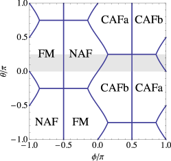
Figure 1: Classical phase diagram of the Hamiltonian defined in Eq. (1) as a function of the frustration angle $\phi$ and the anisotropy parameter $\theta$. For symmetry reasons, it is sufficient to restrict the discussion of the phase diagram to the parameter range $-\pi\leq\phi\leq\pi$, $0\leq\theta\leq\pi/4$ indicated by the shaded area in the figure.

The possible classical phases are ferromagnetic (FM, $\vec{Q}_{\text{FM}}=(0,0)$), Néel antiferromagnet (NAF, $\vec{Q}_{\text{NAF}}=(\pi,\pi)$) and columnar antiferromagnets (CAFa, $\vec{Q}_{\text{CAFa}}=(\pi,0)$, CAFb, $\vec{Q}_{\text{CAFb}}=(0,\pi)$). The latter are degenerate for the isotropic ($J_{1a}=J_{1b}$) case with $\theta=\pi/4$ or $\theta=-3\pi/4$. Fig. 1 displays a sketch of the classical phase diagram in the $\phi$-$\theta$-plane. The shaded stripe in the plot denotes the parameter range $-\pi\leq\phi\leq\pi$, $0\leq\theta\leq\pi/4$ which can be mapped onto the whole phase diagram applying discrete symmetry operations under which the Hamiltonian (1) is invariant.

Ref. Schmidt et al., 2010 and references cited therein contain a thorough discussion of the classical phases and a spin-wave analysis of the ground-state properties of the Hamiltonian (1). In particular, the inherent frustration leading to quantum fluctuations and possible moment reduction is investigated in detail. It is found that the staggered moment is stabilized in the columnar phases by introducing a spatial anisotropy, and a strong influence of frustration on the size of the moment can be excluded. However, linear spin-wave analysis a priori is a semiclassical theory, and naturally the question arises to what extent these results can be confirmed by strictly quantum-mechanical methods. An unbiased but technically more involved approach is to determine the ground-state properties of the Hamiltonian (1) by exact diagonalization on small finite tiles with periodic boundary conditions and to extrapolate the results to the thermodynamic limit using a scaling analysis.

III Technical prerequisites for a finite-size scaling analysis

The most difficult aspect of finite size cluster calculations is the implementation of an efficient finite size scaling procedure to obtain reliable values of physical quantities in the thermodynamic limit. In this section we present in detail the necessary ingredients. We describe how we generate lattice tilings used for exact diagonalization, classify them according to a newly introduced concept of their compactness or squareness (which will be defined later), their point-group symmetry, and their compatibility with the classical phases of our model. These properties allow us to discriminate systematically the various clusters according to their usefulness for the finite size scaling analysis which is of central importance to obtain reliable results. Furthermore we will discuss the derivation of the set of wave vectors associated with a given tile and describe two different finite-size scaling procedures to calculate the ordered moment.

III.1 Tiling the square lattice

For a finite-size scaling analysis, it is common practice to select tiles according to certain geometrical or topological properties. We first briefly describe three different schemes applied in the past to $S=1/2$ spin models before turning to the more general selection scheme used in this paper.

Haan et al. Haan et al. (1992) discuss the $S=1/2$ nearest-neighbor Heisenberg antiferromagnet with helical boundary conditions and define an asymmetry parameter $A=|\ell_{1}-\ell_{2}|/(\ell_{1}+\ell_{2})$, where $\ell_{i}$ are the lengths of the edge vectors of the tiles under consideration. A square-shaped tile (considered as “good”) has $A=0$, but this is true for general diamond-shaped tiles, too. Those tiles having “small $A$” are selected for scaling.

Restricting to strictly square-shaped tiles having at least ${\cal C}_{4}$ point-group symmetry is the recipe used by Schulz et al. Schulz et al. (1996) for discussing ground-state energy and ordered moment of the $S=1/2$ antiferromagnetic $J_{1}-J_{2}$ model. However, with this criterion only very few (two to four) tiles are eventually used for a linear least-squares fit.

Another approach can be found in Ref. Betts et al., 1999, discussing the $S=1/2$ nearest-neighbor $XY$ and Heisenberg antiferromagnets with periodic boundary conditions. The authors introduce a parameter called the topological imperfection of a tile, where a topologically perfect tile is defined as follows: A given lattice point on a tile contains $n_{1}$ nearest neighbors, $n_{2}$ next-nearest neighbors, and so on, up to the $i_{\text{max}}$th-nearest neighbors where the sum over the $n_{i}$ reaches the tile area $N$. (Distance is measured as the minimal number of hops needed to get from one point to another.) If for all $i<i_{\text{max}}$ we have $n_{i}=4i$, which is the number of $i$th-nearest neighbors on the infinite lattice, a tile is considered as topologically perfect. This concept is then extended to the notion of topologically perfect bipartite Néel lattices, i. e., the same conditions as described above are applied individually to each of the two sublattices for antiferromagnetic Néel order. However, tiles are eventually chosen by hand in order to achieve a smooth finite-size scaling behavior of the ground-state energy per site and the square of the magnetization or staggered moment, respectively.

The examples given above are in no way exhaustive, but illustrate one problem common to any finite-size scaling analysis, which becomes particularly apparent when applied to the full phase diagram of the $J_{1a,b}$-$J_{2}$ model. Firstly, only very few tilings might survive the final selection, making a linear two-parameter $\chi^{2}$ fit to the ground-state energy or squared ordered moment of the $J_{1a,b}$-$J_{2}$ model questionable, not to speak about higher-order correction terms included in the fitting procedure. Hasenfratz and Niedermayer (1993)

Secondly, the selection contains some arbitrariness which in our case would lead to selecting different tiles for scaling for different sets of exchange parameters, even within the same classical phase.

Thirdly, given the edge vectors $\vec{a}_{i}$ of a particular parallelogram, this is not a unique way to tile the square lattice. For example, upon replacing $\vec{a}_{1}$ by, say $2\vec{a}_{2}-\vec{a}_{1}$, we get a new tile with identical area which leads to an identical structure of the resulting torus when introducing periodic boundary conditions. Even worse: In general, there are many possible generator matrices $M=(\vec{a}_{1},\vec{a}_{2})$ of the same lattice tiling $\Lambda_{M}$.

However a more systematic approach to select tilings is possible. We will describe this scheme here and employ it for the $J_{1a,b}$-$J_{2}$ model.

A basic requirement is a unique description of the lattice tilings. Schrijver (1986); Domich et al. (1987); Lyness et al. (1991); Stewart et al. (1997) To achieve this, we need some definitions. First, we introduce unimodular matrices $U$, which are defined as integer matrices of dimension $s$ with determinant $\pm 1$. Let us further denote with $U^{(i,j)}$ a unit matrix modified by having a single additional nonzero unit element at position $(i,j)$, and introduce $S^{(i)}$ as a unit matrix modified by having the $(i,i)$th element replaced by $-1$. The unimodular matrices of dimension $s$ form a (non-abelian) group $U_{\text{s}}$ under matrix multiplication, and the generators of this group can be the elements $U^{(i,j)}$ and $S^{(i)}$.

We need another definition: A $s\times s$ integer matrix $H=\left(h_{ij}\right)$ is in Hermite Normal Form (HNF) if and only if

$$h_{ii}\geq 1, i=1\ldots s,$$

$$h_{ij}=0, 1\leq j<i\leq s,$$ (3)

$$h_{ij}\in\left[0,h_{ii}\right), 1\leq i<j\leq s.$$

It can be shown Schrijver (1986) that (a) an arbitrary nonsingular integer matrix $M$ can be uniquely represented by a unimodular matrix $U$ and an HNF matrix $H$ such that

$$U\cdot M=H,$$ (4)

and (b) that for two HNF matrices $H$ and $H^{\prime}$ generating the lattice tilings $\Lambda_{H}$ and $\Lambda_{H^{\prime}}$, we have

$$\Lambda_{H}\equiv\Lambda_{H^{\prime}}\leftrightarrow H=H^{\prime}.$$ (5)

In this way, we can uniquely represent an arbitrary lattice tiling of any given primitive Bravais lattice.

The two-dimensional HNF matrices $H$ have the form

$$H=\left(\begin{array}[]{cc}h_{11}&h_{12}\\ 0&h_{22}\end{array}\right)$$ (6)

representing tiles with the special edge vectors $\vec{h}_{1}=\left(h_{11},h_{12}\right)$ and $\vec{h}_{2}=\left(0,h_{22}\right)$ and area or number of sites $N=h_{11}h_{22}$. For numerical purposes, it would already be sufficient to implement an algorithm using only Eqs. (3) and (6) for building the list of possible tilings.

III.2 Compact tiles

In the spirit of Ref. Schulz et al., 1996, where only square-shaped tiles have been used, we want to generalize this concept and utilize the notion of “squareness” or “compactness” of a tile for selecting the proper tiles for finite-size scaling. For this purpose, we introduce a parameter

$$\rho(M) = \frac{\left|\mathop{\rm Det}M\right|}{\left|\left|M\right|\right|},$$

$$\left|\left|M\right|\right| = \left(\frac{1}{s}\sum_{i=1}^{s}\sqrt{\mathop{\rm Det}\left(M_{i}^{T}M_{i}\right)}\right)^{s/(s-1)}$$ (7)

for a nonsingular integer $s\times s$ matrix $M$, where $M_{i}$ is the (non-square) matrix formed by dropping the $i$th row of $M$. $\rho(M)$ measures the “compactness” (“squareness” in two spatial dimensions) of the $s$-dimensional parallelotope spanned by the row vectors of $M$: We have $0<\rho(M)\leq 1$, and $\rho(M)=1$ if and only if $M$ describes an $s$-dimensional cube, which we regard as the most compact lattice tiling in dimension $s$.

However, calculating $\rho(H)$ for the HNF representation of a lattice tiling is not very useful: According to Eq. (4), a single HNF matrix $H$ represents a whole class ${\cal C}_{H}$ of tiles with matrix representation $M$ which all lead to an identical lattice tiling $\Lambda_{H}=\Lambda_{M}$. But in general, two matrices $M\neq M^{\prime}$ with $\Lambda_{M}=\Lambda_{M^{\prime}}$ have $\rho(M)\neq\rho(M^{\prime})$. From each ${\cal C}_{H}$, we therefore have to choose a tile which has the maximum compactness of all tiles of its class,

$$M_{\text{c}}=M:\rho(M)=\max_{{\cal T}\in{\cal C}_{H}}\left(\rho(M_{{\cal T}})\right)$$ (8)

and assign $\rho(M_{\text{c}})$ to the HNF representant $H=UM_{\text{c}}$ of its class ${\cal C}_{H}$.

With this scheme, we find 816 different classes of tiles with size $N$ between $8$ and $32$. It is impossible to list all of them in this article. Instead, to illustrate the principle we display in Fig. 19 of Appendix A a list of all possible distinct ways to tile the square lattice using tiles of just the smallest useful size $N=8$.

To label the tiles in a unique way, we use the scheme $N$:$h_{11}$-$h_{12}$, where $N$ is the number of sites or tile area and $h_{ij}$ are the coordinates of the first edge vector of the HNF representation of a tile. The eight-site square for example has the label $8$:$2$-$2$ (Fig. 19, third from below).

III.3 Construction of the Brillouin zone for a finite lattice tiling

To reduce the size of the matrices representing the Hamiltonian, it is useful to work with a basis reflecting the periodicity of the lattice, i. e., we construct Bloch states from the states of the $(N,S_{z})$ basis by applying Bloch’s theorem. Algorithmically, the states of the original spinor product basis are collected into classes of wave functions which related to each other by translations with translation vector $\vec{r}$ and associated phase factor ${\rm e}^{{\rm i}\vec{k}\vec{r}}$.

For the finite tilings we are using, the possible wave vectors $\vec{k}$ can assume only certain values. In this section, we discuss how to determine these wave vectors which are contained in the (first) Brillouin zone for a given lattice tiling. We use the fact that a translation by a reciprocal lattice vector will not change the phase of a wave function, as required by Bloch’s theorem. We construct the first Brillouin zone such that the origin is located in one of its corners. This is different from the commonly used Wigner-Seitz construction for infinite lattices, where the origin is in the center of the Brillouin zone. We cannot apply the Wigner-Seitz construction directly to an arbitrary finite lattice, because we require the wave vector $\vec{k}=0$ to be part of the set of reciprocal lattice points generated, and the geometrical center of a given reciprocal lattice tile constructed as described here does not necessarily have a wave vector associated with it.

For the edge vectors $\vec{a}_{1}$ and $\vec{a}_{2}$ of a tile and the corresponding basis vectors $\vec{b}_{1}$ and $\vec{b}_{2}$ of the reciprocal lattice, we get from the orthogonality condition

$$\vec{b}_{1}=\frac{2\pi}{N}\left(a_{22}\atop{-a_{21}}\right),\quad\vec{b}_{2}=\frac{2\pi}{N}\left({-a_{12}}\atop a_{11}\right)$$ (9)

with integer coefficients $a_{ij}$, where

$$N=\left|\mathop{\rm Det}\left(\vec{a}_{1},\vec{a}_{2}\right)\right|$$ (10)

is the number of sites or area of the tile under consideration. The reciprocal lattice vectors $\vec{G}_{1}=2\pi\vec{e}_{x}$ and $\vec{G}_{2}=2\pi\vec{e}_{y}$, where $\vec{e}_{x,y}$ are the Cartesian unit vectors, are given by

$$\vec{G}_{i}=a_{1i}\vec{b}_{1}+a_{2i}\vec{b}_{2},\quad i=1,2$$ (11)

in terms of the reciprocal basis vectors. Within this coordinate system, the reciprocal lattice vectors $\vec{G}_{1}$ and $\vec{G}_{2}$ span the parallelogram making up the first Brillouin zone, which contains exactly $N$ wave vectors $\vec{k}=k_{1}\vec{b}_{1}+k_{2}\vec{b}_{2}$ with integer coefficients $k_{i}$.

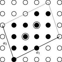
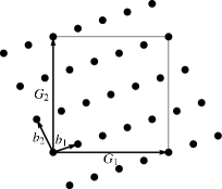
Figure 2: Tile 14:1-11 in direct space (left), and the corresponding reciprocal lattice (right) according to Eqs. (9) and (11). The two circles on the left-hand side mark the two equivalent points of the tile with maximum distance to the origin. Also shown is the first Brillouin zone of the lattice with edge vectors (reciprocal lattice vectors) $\vec{G}_{1}$ and $\vec{G}_{2}$.

These wave vectors can be found with the following criterion: The projections of $\vec{k}$ onto the reciprocal lattice vectors $\vec{G}_{i}$ must be positive semidefinite (we put the origin $(k_{1},k_{2})=(0,0)$ into the lower left corner of the Brillouin zone) and less than the length of the latter, i. e., $0\leq\vec{k}\cdot\vec{G}_{i}<\vec{G}_{i}\cdot\vec{G}_{i}=4\pi^{2}$. With the expressions above for the basis vectors $\vec{b}_{i}$ and the reciprocal lattice vectors $\vec{G}_{i}$, we find as our defining relations for possible wave vectors $\vec{k}$

$$0\leq\mathop{\rm Det}(\vec{k},\vec{G}_{2})<N\ \wedge\ 0\leq-\mathop{\rm Det}(\vec{k},\vec{G}_{1})<N,$$ (12)

writing the column vectors $\vec{G}_{i}$ and $\vec{k}$ in the coordinate system spanned by the basis vectors $\vec{b}_{i}$. Conditions (12) specify exactly $N$ wave vectors $\vec{k}=k_{1}\vec{b}_{1}+k_{2}\vec{b}_{2}$. Fig. 2 illustrates this procedure for tile number 14:1-11.

III.4 Space group symmetry

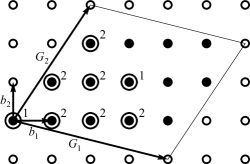
Figure 3: Reciprocal lattice tile 14:1-11. The graphics shows the same tile as in the right-hand side of Fig. 2 corresponding to the first Brillouin zone, but here in the coordinate system spanned by the reciprocal basis vectors $\vec{b}_{1}$ and $\vec{b}_{2}$, indicated by the short arrows. The dotted circles denote the irreducible wedge of the Brillouin zone (tile 14:1-11 has ${\cal C}_{2}$ symmetry only), numbers give the size of the star of the corresponding wave vector.

To avoid unnecessary computations, we calculate Lanczos eigensystems only at those wave vectors $\vec{k}$ which are not related by a space group operation. Therefore we have to determine the irreducible wedge of the Brillouin zone. Figure 3 illustrates this for tile 14:1-11, which has ${\cal C}_{2}$ point group symmetry: The number of wave vectors is reduced from a total of 14 to eight nonequivalent ones. The small numbers in the figure denotes the size of the star of the corresponding wave vector.

Since we are working with mappings of the full tile, it is useful to work in a coordinate system of the reciprocal lattice vectors $\vec{G}_{1}$ and $\vec{G}_{2}$. For the projection of an arbitrary wave vector $\vec{k}=\hat{k}_{1}\vec{G}_{1}+\hat{k}_{2}\vec{G}_{2}$ (not necessarily located in the first Brillouin zone) onto the reciprocal lattice vectors, we have

$$\hat{k}_{1} = \frac{\vec{k}\cdot\vec{G}_{1}}{|\vec{G}_{1}|^{2}}=\frac{1}{N}\mathop{\rm Det}\left(\vec{k},\vec{G}_{2}\right),$$ (13)

$$\hat{k}_{2} = \frac{\vec{k}\cdot\vec{G}_{2}}{|\vec{G}_{2}|^{2}}=-\frac{1}{N}\mathop{\rm Det}\left(\vec{k},\vec{G}_{1}\right)$$ (14)

(compare Eq. (12)). Note the minus sign in the last equation and the interchange of $\vec{G}_{1}$ and $\vec{G}_{2}$: The projection of $\vec{k}$ onto $\vec{G}_{1}$ is proportional to the area of the parallelogram spanned by $\vec{k}$ and $\vec{G}_{2}$ and vice versa.

We can write

$$\hat{k}_{i}=\frac{n_{i}}{N}+m_{i},\quad 0\leq n_{i}<N,\quad m_{i}\in\mathbb{Z}$$ (15)

for the coefficients of a wave vector $\vec{k}=M\cdot\vec{q}$ resulting from the application of a space group operation $M$ onto a wave vector $\vec{q}$ in the first Brillouin zone. Mapping $\vec{k}$ back into the first Brillouin zone amounts to setting $m_{i}=0$ in the equation above. This gives us a convenient and numerically well defined procedure for mapping the Brillouin zone onto its irreducible part.

III.5 Ordered ground states

The classical $J_{1a,b}$-$J_{2}$ model on the square lattice has four ground states with ordering wave vectors $\vec{Q}=(0,0)$, $(\pi,\pi)$, and $\vec{Q}=(\pi,0)$ or $(0,\pi)$. Although in the quantum case the corresponding wave functions, except for the ferromagnet, are not eigenstates of the Hamiltonian, it is important that the tilings of the infinite lattice are chosen such that these states corresponding to the classically ordered phases are not suppressed when applying periodic boundary conditions.

We can determine those tiles compatible with a classical ground state by applying a test for the existence of the corresponding classical ordering vector $\vec{Q}$ in the list of wave vectors for a given tile,

$$n_{1}\vec{b}_{1}+n_{2}\vec{b}_{2}=\vec{Q},\quad n_{i}\in\mathbb{Z}.$$ (16)

From Eqs. (9), we get

$$\frac{2\pi}{N}\left[n_{1}\left(a_{22}\atop{-a_{21}}\right)+n_{2}\left({a_{12}}\atop a_{11}\right)\right]=\left(Q_{1}\atop Q_{2}\right),$$ (17)

which has to be fulfilled for integer coefficients $n_{i}$.

• Ferromagnet: $\vec{Q}_{\text{FM}}=(0,0)$. Since we have chosen the phase of our wave functions such that $\vec{k}=0$ is always a valid wave vector, all tiles are compatible with the ferromagnet.

• CAFa phase: $\vec{Q}_{\text{CAFa}}=(\pi,0)$, and we have

  $$n_{1}=\frac{a_{11}}{2},\quad n_{2}=\frac{a_{21}}{2}.$$ (18)

  Stated physically, the Mannheim distance (or Manhattan distance) $d_{\text{M}}(\vec{p}_{1},\vec{p}_{2})=\sum_{i}\left|p_{1i}-p_{2i}\right|$, counting the minimal number of hops on the lattice needed to get from one point to another, of any two points $\vec{p}_{i}$ and $\vec{p}_{j}$ belonging to the same sublattice projected onto the $x$ direction of the lattice must be even,

  $$d_{x}(\vec{p}_{i},\vec{p}_{j})=|p_{jx}-p_{ix}|\equiv 2n,\ n\in\mathbb{N}_{0}.$$ (19)

• CAFb phase: $\vec{Q}_{\text{CAFb}}=(0,\pi)$. We get from condition (17)

  $$n_{1}=\frac{a_{12}}{2},\quad n_{2}=\frac{a_{22}}{2},$$ (20)

  so the components $a_{12}$ and $a_{22}$ parallel to $\vec{e}_{y}$ must be even numbers. For completeness, the appropriate condition is given by

  $$d_{y}(\vec{p}_{i},\vec{p}_{j})\equiv 2n,\ n\in\mathbb{N}_{0}$$ (21)

  for any two lattice points $\vec{p}_{i}$ and $\vec{p}_{j}$ with $S_{i}^{z}=S_{j}^{z}$.

• Néel phase: $\vec{Q}_{\text{NAF}}=(\pi,\pi)$. Eq. (17) can be solved with

  $$n_{1}=\frac{a_{11}+a_{22}}{2},\quad n_{2}=\frac{a_{21}+a_{22}}{2}.$$ (22)

  This is equivalent to

  $$d_{\text{M}}(\vec{p}_{i},\vec{p}_{j})\equiv 2n,\ n\in\mathbb{N}_{0}$$ (23)

  for any two lattice points $\vec{p}_{i}$ and $\vec{p}_{j}$ on the same sublattice.

• All four phases: All components of the edge vectors $\vec{a}_{1}$ and $\vec{a}_{2}$ must be even individually in order to be compatible with the full set of classical phases.

In this way, we can classify any given lattice tiling with respect to the classical phases it belongs to.

III.6 Selection of tiles

$$\begin{array}[]{cccccccccc}\text{Tile}&\text{NAF}&\text{CAFa}&\text{CAFb}&\Box&{\cal C}_{2}&{\cal C}_{2V\,\text{rect}}&{\cal C}_{2V\,\text{dia}}&{\cal C}_{4}&{\cal C}_{4V}\\ \hline\cr\text{\bf\text@underline{8:2-2}}&\bullet&\bullet&\bullet&\text{ 1.000}&\bullet&\bullet&\bullet&\bullet&\bullet\\ \hline\cr\text{10:1-3}&\bullet&-&-&\text{ 1.000}&\bullet&-&-&\bullet&-\\ \text{10:1-4}&-&-&\bullet&\text{ 0.966}&\bullet&-&-&-&-\\ \text{10:2-2}&-&\bullet&-&\text{ 0.966}&\bullet&-&-&-&-\\ \hline\cr\text{12:3-0}&-&-&\bullet&\text{ 0.980}&\bullet&\bullet&-&-&-\\ \text{12:4-0}&-&\bullet&-&\text{ 0.980}&\bullet&\bullet&-&-&-\\ \text{12:1-5}&\bullet&-&-&\text{ 0.960}&\bullet&-&\bullet&-&-\\ \text{\bf\text@underline{12:2-2}}&\bullet&\bullet&\bullet&\text{ 0.901}&\bullet&-&-&-&-\\ \hline\cr\text{14:1-3}&\bullet&-&-&\text{ 0.961}&\bullet&-&-&-&-\\ \text{14:1-4}&-&-&\bullet&\text{ 0.938}&\bullet&-&-&-&-\\ \text{14:2-3}&-&\bullet&-&\text{ 0.938}&\bullet&-&-&-&-\\ \hline\cr\text{\bf\text@underline{16:4-0}}&\bullet&\bullet&\bullet&\text{ 1.000}&\bullet&\bullet&\bullet&\bullet&\bullet\\ \hline\cr\text{18:3-3}&\bullet&-&-&\text{ 1.000}&\bullet&\bullet&\bullet&\bullet&\bullet\\ \text{18:1-4}&-&-&\bullet&\text{ 0.975}&\bullet&-&-&-&-\\ \text{18:2-4}&-&\bullet&-&\text{ 0.975}&\bullet&-&-&-&-\\ \hline\cr\text{\bf\text@underline{20:2-4}}&\bullet&\bullet&\bullet&\text{ 1.000}&\bullet&-&-&\bullet&-\\ \hline\cr\text{22:1-6}&-&-&\bullet&\text{ 0.981}&\bullet&-&-&-&-\\ \text{22:2-4}&-&\bullet&-&\text{ 0.981}&\bullet&-&-&-&-\\ \text{22:1-5}&\bullet&-&-&\text{ 0.961}&\bullet&-&-&-&-\\ \hline\cr\text{24:1-10}&-&-&\bullet&\text{ 0.988}&\bullet&-&-&-&-\\ \text{24:2-5}&-&\bullet&-&\text{ 0.988}&\bullet&-&-&-&-\\ \text{24:1-7}&\bullet&-&-&\text{ 0.980}&\bullet&-&\bullet&-&-\\ \text{\bf\text@underline{24:4-0}}&\bullet&\bullet&\bullet&\text{ 0.960}&\bullet&\bullet&-&-&-\\ \hline\cr\text{26:1-5}&\bullet&-&-&\text{ 1.000}&\bullet&-&-&\bullet&-\\ \text{26:1-10}&-&-&\bullet&\text{ 0.964}&\bullet&-&-&-&-\\ \text{26:2-5}&-&\bullet&-&\text{ 0.964}&\bullet&-&-&-&-\\ \hline\cr\text{28:1-8}&-&-&\bullet&\text{ 0.986}&\bullet&-&-&-&-\\ \text{28:4-3}&-&\bullet&-&\text{ 0.986}&\bullet&-&-&-&-\\ \text{\bf\text@underline{28:2-4}}&\bullet&\bullet&\bullet&\text{ 0.961}&\bullet&-&-&-&-\\ \hline\cr\text{30:5-0}&-&-&\bullet&\text{ 0.992}&\bullet&\bullet&-&-&-\\ \text{30:6-0}&-&\bullet&-&\text{ 0.992}&\bullet&\bullet&-&-&-\\ \text{30:1-5}&\bullet&-&-&\text{ 0.974}&\bullet&-&-&-&-\\ \hline\cr\text{\bf\text@underline{32:4-4}}&\bullet&\bullet&\bullet&\text{ 1.000}&\bullet&\bullet&\bullet&\bullet&\bullet\end{array}$$

Table 1: Label, classical phase compatibility, squareness, and point groups for selected lattice tilings between 8 and 32 sites. For each even area $N$ and for each classical phase, the list contains the compatible tile with maximum squareness as defined in Eq. (7). For $N=12$ and $24$, the tiles compatible with all classical phases are included, too, although they have a comparatively small squareness. The tile labels have the form $N$:$h_{11}$-$h_{12}$, where $h_{1j}$ are the components of the first edge vector of a tile in HNF representation. Those tiles compatible with all four classical phases, required for the discussion of the spatially isotropic model with columnar order, are underlined and typeset in bold.

In order to discuss spatial anisotropies, we do not regard lattice tilings as equivalent which are related by a point-group operation on the square lattice. An example would be the four different tiles 8:1-2, 8:1-6, 8:2-1, and 8:2-3, see Fig. 19. In this way, we get $816$ different tilings of the square lattice with tiles between $8$ and $32$ sites. Out of these, we select, for each even tile area and for each classical phase, the tile having the maximum squareness. In addition, for $N=4\ell$, $\ell\in\mathbb{N}$, we include the tile with maximum squareness containing both CAFa and CAFb ordering vectors, which is equivalent to containing all four classical ordering vectors. These special tiles are of particular importance for the spatially isotropic model, due to the degeneracy of the two columnar phases in this case. The resulting list is displayed in Table 1. Each line contains the tile label, its compatibility with classical phases (Sect. III.5), its squareness (Sect. III.2), and its point group symmetry (Sect. III.4).

For the ${\cal C}_{2V}$ group, two sets of mirror “planes” exists: The point group ${\cal C}_{4V}$ contains two isomorphic subgroups ${\cal C}_{2V\,\text{rect}}$ and ${\cal C}_{2V\,\text{dia}}$, corresponding to a tile with either a rectangular shape (mirror planes parallel to the edges) or a diamond-like shape (mirror planes along the diagonals). This distinction is important when discussing orthorhombic or trigonal symmetry breaking, since ${\cal C}_{4V}$ is reduced to the respective ${\cal C}_{2V}$ symmetry in this case. For simplicity, we also label those tiles having ${\cal C}_{2V}$ but not ${\cal C}_{4V}$ symmetry accordingly in Table 1.

III.7 Static structure factor and ordered moment

In a finite system at zero magnetic field the ground state has $S_{z}=0$ and therefore does not exhibit the spontaneous symmetry breaking of the infinite lattice. The ordered moment $M(\vec{Q})$ rather has to be obtained indirectly from the properly normalized static structure factor according to

$$S_{N}(\vec{Q}) = \frac{1}{\cal N}\sum_{i,j=1}^{N}\left\langle\vec{S}_{i}\vec{S}_{j}\right\rangle{\rm e}^{{\rm i}\vec{Q}\left(\vec{R}_{i}-\vec{R}_{j}\right)}$$

$$= \frac{N}{\cal N}\left[\left\langle\vec{S}_{1}\vec{S}_{1}\right\rangle+\sum_{j=2}^{N}\left\langle\vec{S}_{1}\vec{S}_{j}\right\rangle{\rm e}^{{\rm i}\vec{Q}\left(\vec{R}_{1}-\vec{R}_{j}\right)}\right],$$

where the angular brackets denote the ground-state expectation value in the $S_{z}=0$, $\vec{k}=0$ subspace of the Hilbert space. In the thermodynamic limit, if $\vec{Q}$ is the ordering vector of the corresponding classical phase, we can then identify

$$M^{2}(\vec{Q})=\lim_{N\to\infty}M^{2}_{N}(\vec{Q})=\zeta(\vec{Q})\lim_{N\to\infty}S_{N}(\vec{Q})$$ (25)

with the appropriate normalization $\cal N$ of $S_{N}(\vec{Q})$. Here we have introduced a factor

$$\zeta(\vec{Q})=\left\{\begin{array}[]{cl}1,&\vec{Q}=0\ \mbox{or}\ (\pi,\pi)\\ 2,&\vec{Q}=(\pi,0)\ \mbox{or}\ (0,\pi)\end{array}\right.$$ (26)

to account for the additional lattice rotation symmetry breaking in the CAFa and CAFb phases. Schulz et al. (1996)

For a perfectly ordered classical state with wave vector $\vec{Q}$, the ordered moment assumes its maximum value, $M(\vec{Q})=S$, and we have

$$\left\langle\vec{S}_{i}\vec{S}_{j}\right\rangle=\left\langle S_{i}^{z}S_{j}^{z}\right\rangle=S^{2}{\rm e}^{-{\rm i}\vec{Q}\left(\vec{R}_{i}-\vec{R}_{j}\right)},\quad i\neq j.$$ (27)

Assuming perfect order for the finite tile under consideration, too, we have

$$S_{N}(\vec{Q}) = \frac{N}{\cal N}\left[S(S+1)+(N-1)S^{2}\right]$$ (28)

$$= \frac{1}{\cal N}\ NS\left(NS+1\right).$$

If we require $S_{N}(\vec{Q})=S^{2}$ also in this case, we have to set

$${\cal N}=N\left(N+\frac{1}{S}\right),$$ (29)

which is the normalization we use for any tile included into our finite-size scaling analysis for $M_{N}(\vec{Q})$. This is in accordance with Refs. Schulz et al., 1996; Bernu et al., 1994, and slightly deviates from the ${\cal N}=N^{2}$ normalization commonly used by many authors.

In the FM regime, although the fully polarized (all-up) state is an eigenstate of the Hamiltonian, the structure factor at the antiferromagnetic ordering vectors remains small, but finite. Assuming perfect order again, we get for the individual terms in the sum Eq. (III.7)

$$\left\langle\vec{S}_{1}\vec{S}_{1}\right\rangle=S(S+1),\quad\left\langle\vec{S}_{1}\vec{S}_{j}\right\rangle=S^{2},\quad j\neq 1,$$ (30)

leading to

$$S_{N}(\vec{Q})=\frac{N}{\cal N}\left[S(S+1)+S^{2}\sum_{j=2}^{N}{\rm e}^{-{\rm i}\vec{Q}\vec{R}_{j}}\right].$$ (31)

Let us restrict to tiles with an even area $N$ which is a necessary condition for being compatible with at least one of the non-FM phases of the $J_{1a,b}$-$J_{2}$ model. The sum in the above equation contains only exponentials which can acquire the values $+1$ or $-1$ for $\vec{Q}=(\pi,\pi)$, $(\pi,0)$, or $(0,\pi)$. For each of these three wave vectors, there are $N/2$ sites $j$ with distance $\vec{R}_{j}$ to site $1$ which have phase $+1$, and $N/2$ sites with phase $-1$. Site $1$ obviously belongs to the former, such that we have $N/2-1$ terms left in the sum over the exponentials above having phase $+1$, and we get

$$\sum_{j=2}^{N}{\rm e}^{-{\rm i}\vec{Q}\vec{R}_{j}}=\left(\frac{N}{2}-1\right)\times(+1)+\frac{N}{2}\times(-1)=-1.$$ (32)

With $\cal N$ given by Eq. (29), we therefore have

$$S_{N}(\vec{Q})=\frac{S}{N+1/S}$$ (33)

for all three antiferromagnetic wave vectors in the ferromagnetic phase. As required, this value vanishes in the thermodynamic limit.

III.8 Long-distance correlations

An alternative way of calculating the ordered moment in the thermodynamic limit is mentioned for example in Refs. Bernu et al., 1994; Sandvik, 1997: For the infinite system, in an ordered phase with a staggered moment, the spin correlation function factorizes for large distances $|\vec{R}_{i}-\vec{R}_{j}|$, and Eq. (27) simplifies:

$$\lim_{\left|\vec{R}_{i}-\vec{R}_{j}\right|\to\infty}\left|\left\langle\vec{S}_{i}\vec{S}_{j}\right\rangle\right|=\left|\left\langle\vec{S}_{i}\right\rangle\left\langle\vec{S}_{j}\right\rangle\right|=M^{2}(\vec{Q}).$$ (34)

Working with a finite compact tile, we can extrapolate the spin correlation function for a single pair of spins, defining lattice points $i$ and $j$ such that their distance on the tile is maximized under given periodic boundary conditions. Without loss of generality, we can restrict ourselves to finding the pair $(1,j)$ or just site $j$ being maximally apart from the origin.

We have to define a metric on a tile reflecting the periodic boundary conditions: Each tile has four corners with coordinates $(0,0)$, $\vec{a}_{1}$, $\vec{a}_{2}$, and $\vec{a}_{1}+\vec{a}_{2}$, which are all equivalent to point $1$. Using the Mannheim distance $d_{\text{M}}$ again, we define the toroidal Mannheim distance between two points $\vec{R}_{i}$ and $\vec{R}_{j}$ on a tile as

$$d_{\text{T}}(i,j)=\min\left\{d_{\text{M}}\left(\vec{R}_{ij},0\right),d_{\text{M}}\left(\vec{R}_{ij},\vec{a}_{1}\right),d_{\text{M}}\left(\vec{R}_{ij},\vec{a}_{2}\right),d_{\text{M}}\left(\vec{R}_{ij},\vec{a}_{1}+\vec{a}_{2}\right)\right\}$$ (35)

yielding the minimal distance between two points $\vec{R}_{i}$ and $\vec{R}_{j}$ on a torus. Here the vector $\vec{R}_{ij}$ is the point emerging from $\vec{R}_{j}-\vec{R}_{i}$ when shifting $\vec{R}_{i}$ to the origin, projected back into the original tile: With

$$\vec{R}_{j}-\vec{R}_{i} = \left(x_{j1}-x_{i1}\right)\vec{a}_{1}+\left(x_{j2}-x_{i2}\right)\vec{a}_{2}$$ (36)

$$= \frac{1}{N}\left[\left(n_{j1}-n_{i1}\right)\vec{a}_{1}+\left(n_{j2}-n_{i2}\right)\vec{a}_{2}\right]$$

this point is simply given by

$$\vec{R}_{ij} = \frac{1}{N}\left[\left(\left(n_{j1}-n_{i1}\right)\mathop{\rm mod}N\right)\vec{a}_{1}\right.$$

$$\phantom{\frac{1}{N}}\left.+\left(\left(n_{j2}-n_{i2}\right)\mathop{\rm mod}N\right)\vec{a}_{2}\right].$$

With respect to the distance $d_{\text{T}}$, we can then define

$$\tilde{M}_{N}^{2}(\vec{Q})=\left|\left\langle\vec{S}_{1}\vec{S}_{j}\right\rangle\right|_{j=\max_{d_{\text{T}}(1,j)}(j\in{\cal T}(N))}.$$ (38)

For a square with size $N=L^{2}$, $L$ even, the point $\vec{R}_{j}=(L/2,L/2)$, i. e., the center of the square, has maximum distance $d_{\text{T}}$ from the origin. However, in most cases, due to the lack of a lattice point located in the geometrical center of the tile, there will be, for even $N$, two sites $j$ having the same maximum distance $d_{\text{T}}$ from the origin, see Fig. 2 for an example. For our calculations, we just select one of them. We then can give an estimate for the ordered moment as

$$M^{2}(\vec{Q})=\lim_{N\to\infty}\tilde{M}_{N}^{2}(\vec{Q}).$$ (39)

IV Finite-size scaling analysis

In Refs. Hasenfratz and Niedermayer, 1993; Sandvik, 1997, the area dependence of ground-state properties of the two-dimensional antiferromagnetic Heisenberg model has been derived using chiral perturbation theory. In particular, for the ground-state energy and the ordered moment, the following scaling behavior has been found:

$$E_{0N} = E_{0}+\beta c\frac{1}{N^{3/2}}+\frac{c^{2}}{4\rho}\frac{1}{N^{2}}+{\cal O}\left(\frac{1}{N^{5/2}}\right),$$ (40)

$$M_{N}^{2}(\vec{Q}) = M^{2}(\vec{Q})+\alpha\frac{M^{2}(\vec{Q})}{c\chi_{\perp}}\frac{1}{N^{1/2}}+{\cal O}\left(\frac{1}{N}\right),$$ (41)

where $c=\sqrt{\rho/\chi_{\perp}}$ is the spin-wave velocity, $\rho$ the spin stiffness constant, and $\chi_{\perp}$ the transverse susceptibility. $\alpha=0.620704$ and $\beta=-1.437745$ are numerical constants.

Although these results were proposed only for the isotropic unfrustrated case, we use them for the whole phase diagram. We argue that the form of the scaling functions should not depend on range and anisotropy of interactions within certain limits, as long as the model belongs to the same universality class. However the individual coefficients in Eqs. (40) and (41) might change. Hence we assume the following size dependences for the ground-state energy and the ordered moment:

$$E_{0N} = E_{0}+\frac{e_{1}}{N^{3/2}}+\frac{e_{2}}{N^{2}},$$ (42)

$$M_{N}^{2}(\vec{Q}) = M^{2}(\vec{Q})+\frac{m_{1}^{2}}{N^{1/2}}+\frac{m_{2}^{2}}{N},$$ (43)

where the latter scaling function is applied to both $M_{N}(\vec{Q})$ and $\tilde{M}_{N}(\vec{Q})$. With the exception of the point $(\phi,\theta)=(0,\pi/4)$ (isotropic nearest-neighbor exchange $J_{1}$ only), for all combinations of $\phi$ and $\theta$ discussed here we use only the first two terms in the equations above for our scaling analysis. This is due to the comparatively small number of different areas of the tiles actually included in the calculation.

We have calculated the ground-state energies $E_{0N}$, structure factors $M_{N}^{2}(\vec{Q})$, and long-distance correlation functions $\tilde{M}_{N}^{2}(\vec{Q})$ at the respective ordering vectors for tilings of $11$ different sizes $N$ between $8$ and $28$ at more than $300$ points in the $(\phi,\theta)$ plane, producing roughly $17\,500$ data sets altogether. To demonstrate the procedure, in the following we show a few examples at some significant points in the phase diagram before presenting our main results in section V.

IV.1 The ground-state energy

The ground-state energy of the Hamiltonian (1) is calculated in the subspace with total spin $S_{z}=0$ at wave vector $\vec{k}=\vec{Q}$ (the respective classical ordering vector) except for tiles with area $N=4\ell$, $\ell\in\mathbb{N}$, where the ground state is found in the $\vec{k}=0$ sector. Figs. 4–6 show the dependence of the ground-state energy per site $E_{0N}$ on the reciprocal area of the tiles for selected model parameters $(\phi,\theta)$. (We plot $-E_{0N}$ in order to be consistent with previous studies Schulz et al. (1996); Betts et al. (1999).) The insets display schematically the position in the phase diagram the plots refer to. Here and in the following, energies are measured in units of $J_{\text{c}}$, unless mentioned otherwise.

The short horizontal dashes show the calculated energies for those tiles compatible with the corresponding classical phases for a given parameter set $(\phi,\theta)$. The energy eigenvalues of those tiles having maximum squareness are indicated by the small open circles. We have also determined $E_{0N}$ for tiles incompatible with the classical phases. In these cases, we get consistently much higher values for $E_{0N}$, and we omit them in the plots. The larger value of the energy for these tilings is due to the fact that the interactions governed by the geometry of the tile prevent achieving a lower value of the energy.

Furthermore there are tiles which are compatible with classical phases but correspond to very skewed parallelograms with small squareness (less than $1/2$), in some cases they are ladders or even chains. They have a much lower ground-state energy (shown as dashes above the scaling line in Figs. 4 and 5) than the tiles of equal size and larger squareness. Although the energies of these finite clusters with low squareness are shown in the figure for completeness they are not used for the scaling procedure.

For each tile area $N$, we have to choose one value for $E_{0N}$ out of the stack of eigenvalues to be included into the finite-size scaling fit applying Eq. (42). According to our selection criteria, we choose the tile which (i) is compatible with the classical phase the parameter set $(\phi,\theta)$ belongs to, and (ii) is the best approximation to a square in the sense of Eq. (7). See Table 1 for a list of them. The values $E_{0N}$ obtained in this way, labeled by the open circles in Figs. 4–6, are then used for a $\chi^{2}$ fit to Eq. (42), indicated by the solid lines in the figures.

IV.1.1 Isotropic nearest-neighbor exchange

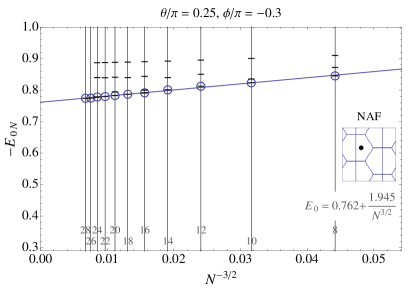
Figure 4: Ground-state energy of the isotropic model as a function of $1/N^{3/2}$. Top: Conventional Néel AF Heisenberg model ($J_{1a}=J_{1b}$, $J_{2}=0$). Bottom: Additional ferromagnetic next-nearest neighbor exchange $J_{2}<0$. The dashes indicate the energy per site for different tilings. Those having maximum squareness, marked with a circle, are used for the scaling and extrapolation. The solid line shows the scaling curve, Eq. (42). The insets in these and the following plots show the parameter position $(\phi,\theta)$ in the phase diagram, cf. Fig. 1. The numbers near the abscissae denote the tile size $N$.

The top of Fig. 4 shows the ground-state energy scaling of the conventional unfrustrated antiferromagnetic Heisenberg model with $J_{1a}=J_{1b}=J_{\text{c}}$ and $J_{2}=0$, equivalent to $(\phi,\theta)=(0,\pi/4)$. We obtain the value $E_{0}=-0.66(5)$ for the extrapolated ground state energy which is in agreement with previous calculations, see, e. g., Refs. Schulz et al., 1996; Betts et al., 1999 and references cited therein. It should be noted that not always the tile having the highest squareness also has the highest ground-state energy compared to the other tiles with the same area $N$. However, the differences are small, and not visible on the scale of Fig. 4.

IV.1.2 Next-nearest neighbors and spatial anisotropy

The lower plot in Fig. 4 shows the scaling of the ground state energy for the point $(\phi,\theta)=(-0.3\pi,\pi/4)$ corresponding to the isotropic model with finite ferromagnetic next-nearest-neighbor exchange $J_{2}$. Ferromagnetic $J_{2}$ stabilizes the $(\pi,\pi)$ order, and we obtain a lower ground state energy $E_{0}=-0.76(2)$ accordingly.

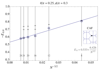
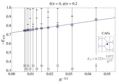
Figure 5: Finite-size scaling of the ground-state energy in (top) the CAF phase of the isotropic and (bottom) the CAFa phase of the maximally anisotropic model for different tilings. Labels, symbols and lines have the same meaning as in Fig. 4.

The top of Fig. 5 illustrates the scaling behavior in the CAF phase of the isotropic model with $(\phi,\theta)=(0.3\pi,\pi/4)$. Here all exchange constants are antiferromagnetic, and the competition between them leads to columnar order. Because $J_{1a}=J_{1b}$ here, we have two equivalent ordering vectors $(\pi,0)$ and $(0,\pi)$, labeled by CAFa and CAFb, respectively. Only the tiles which contain both the CAFa and CAFb classical phases have truly the symmetries required by the Hamiltonian in this case. Consequently only the tiles with size $N=4\ell$, $\ell\in\mathbb{N}$ are acceptable for scaling, and we have much less data points available as compared to the Néel phase, Fig. 4. As before, we select out of these the tiles with maximum squareness for the scaling procedure which leads to a ground state energy $E_{0}=-0.53(2)$.

In the anisotropic case, CAFa and CAFb phases are no longer equivalent. An example of CAFa for the maximally anisotropic case $(\phi,\theta)=(0.2\pi,0)$, where $J_{1b}=0$ and $J_{2}$ antiferromagnetic, is shown in the bottom part of Fig. 5. Here the tiles do not have to be compatible with the $(0,\pi)$ ordering of the CAFb phase, therefore the number of possible tilings is larger. Also the scaling behavior is improved again. Compared to the isotropic case, the extrapolated value for the ground-state energy is lower, indicating that the introduction of a rectangular anisotropy stabilizes the columnar order.

IV.1.3 Magnetically disordered regimes

The scenarios discussed until here have one property in common: All of them have parameter sets $(\phi,\theta)$ which are located deeply inside the corresponding classically ordered phases, and all of them show a good and well-defined scaling behavior of the ground-state energy. (We give a precise definition and discussion of the meaning of “good” and “well-defined” in Sect. IV.3.)

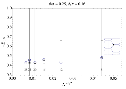
Figure 6: The tile size dependence of the ground-state energy in the disordered regime at the CAF-FM border. In this case a reliable linear scaling result cannot be obtained from the circles.

However, this changes when approaching the disordered regimes at the borders of the columnar phases. Even with our stringent conditions for tile selection, the behavior in the region where the transition from the Néel to the CAF phase occurs is quite different. In fact an area dependence as given by Eq. (42) no longer seems to apply, and the concept of choosing the most-square-like tiles for scaling apparently becomes inappropriate. An example of this behavior is displayed in Fig. 6 corresponding to the well know disordered case of the isotropic model with $J_{2}/J_{1}\approx 1/2$.

Expressed differently, finite-size scaling breaks down and is no longer a useful concept by itself in and near the disordered regions at the edges of the columnar phases in the phase diagram. This will be described in more detail including a discussion of the correlation functions and the ordered moment in section V.

We conclude that a stable finite-size scaling analysis of the ground state energies can be achieved inside the NAF and CAFa,b regions for all frustration and anisotropy parameters provided a careful selection of tiles according to phase compatibility and maximum squareness in each case is carried through. However the scaling analysis cannot be made in the transition regions close to the phase boundaries in Fig. 1. This is correlated with the breakdown of the ordered moment in these regions as will be shown in the next section.

IV.2 Ordered moment, structure factor and correlation function

Using the ground-state wave-function obtained by diagonalizing the Hamiltonian matrix, we calculate the expectation values of the spin correlation functions $\langle\vec{S}_{i}\vec{S}_{j}\rangle$. Subsequently, we calculate the finite-size equivalent $M_{N}^{2}(\vec{Q})$ of the ordered moment applying the two methods described in Sects. III.7 and III.8. In the same way as for the ground-state energy in the previous section, we select the tile with maximum squareness for each tile area $N$ and fit Eq. (43) to the resulting data points. Again, apart from the conventional Néel antiferromagnet we apply a linear scaling only, ignoring the last term in Eq. (43).

IV.2.1 Isotropic nearest-neighbor exchange

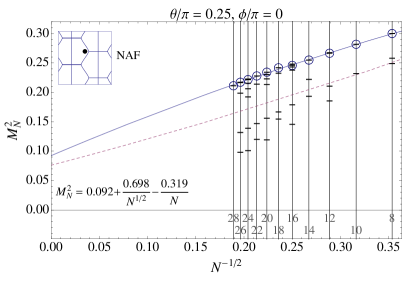
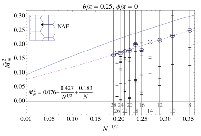
Figure 7: Finite-size scaling of the ordered moment for the isotropic nearest-neighbor AF Heisenberg model for different tilings. Top: $M_{N}^{2}(\vec{Q}_{\text{NAF}})$ derived from the structure factor $S_{N}(\vec{Q}_{\text{NAF}})$. Bottom: $\tilde{M}_{N}^{2}(\vec{Q}_{\text{NAF}})$ derived from the long-distance correlation function. The horizontal dashes and open circles denote the values for different tiles. The latter are those with maximum squareness which are used for the scaling and extrapolation. The solid lines show the fit of Eq. (43) to $M_{N}^{2}(\vec{Q}_{\text{NAF}})$, the dashed lines the fit to $\tilde{M}_{N}^{2}(\vec{Q}_{\text{NAF}})$. To facilitate the comparison, we reproduce both fits in both plots.

The top part of Fig. 7 shows the ordered moment derived from the structure factor, Sect. III.7, the bottom part shows $\tilde{M}^{2}(\vec{Q})$ obtained from the long-distance correlation function, Sect. III.8, for the unfrustrated ($J_{2}=0$) isotropic AF Heisenberg model ($\phi=0,\theta=\pi/4$). As before, the horizontal dashes show the values for different tilings, and the tiles with maximum squareness are indicated by circles. From the top figure it is evident that the most square-like tiles have also the largest structure factor at the ordering vector $\vec{Q}=(\pi,\pi)$ for the NAF phase.

A $\chi^{2}$ fit of Eq. (43) using all three terms has been applied to both $M_{N}^{2}(\vec{Q})$ and $\tilde{M}_{N}^{2}(\vec{Q})$ separately. The solid lines in the two plots of Fig. 7 denote the result of fitting to $M_{N}^{2}(\vec{Q})$, and we get $M(\vec{Q}_{\text{NAF}})=0.30(3)$. This is in good agreement with previous studies Schulz et al. (1996); Sandvik (1997); Betts et al. (1999). The same fit applied to $\tilde{M}_{N}^{2}(\vec{Q})$, indicated by the dashed lines in the figure, gives a slightly lower value $\tilde{M}(\vec{Q}_{\text{NAF}})=0.27(6)$ for the thermodynamic limit. We believe this to be a good indicator for the accuracy within which we can determine asymptotic values for the ordered moment. Also the relative error (to be explained below) is larger for the latter method, which is a consequence of the fact that only a single correlation function is evaluated, while in the first method, a Fourier transform using all possible $\langle\vec{S}_{i}\vec{S}_{j}\rangle$ is taken.

IV.2.2 Next-nearest neighbors and spatial anisotropy

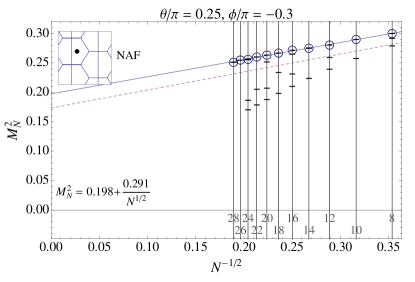
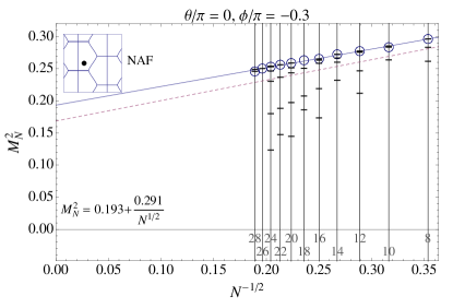
Figure 8: Finite-size scaling of the ordered moment in the NAF phase with ferromagnetic $J_{2}$. Top: isotropic model, $J_{1a}=J_{1b}$. Bottom: maximally anisotropic case, $J_{1b}=0$. The horizontal dashes denote $M_{N}^{2}(\vec{Q})$ for different tilings, the solid lines are fits with Eq. (43) to the values for most-square-like-tiles, marked with a circle. Results for $\tilde{M}_{N}^{2}(\vec{Q})$ for individual tiles are not shown, fits to $\tilde{M}_{N}^{2}(\vec{Q})$ are displayed as the dashed lines.

The ordered moment scaling for ferromagnetic $J_{2}<0$ ($\phi=-0.3\pi$), both in the isotropic ($J_{1a}=J_{1b}$) and maximally anisotropic ($J_{1b}=0$) case is shown in the top and bottom of Fig. 8 respectively. The horizontal dashes denote $M_{N}^{2}(\vec{Q})$ for individual tilings, the solid line represents a fit with Eq. (43) to the values for most-square-like-tiles (circles in the plot). The dashed lines denote fits to $\tilde{M}_{N}^{2}(\vec{Q})$ for the same set of tiles. (Individual values are not shown.) Again, a comparison of the extrapolated values for $M^{2}(\vec{Q})$ from the two different scaling procedures can serve as an indicator of the quality of the finite-size scaling analysis.

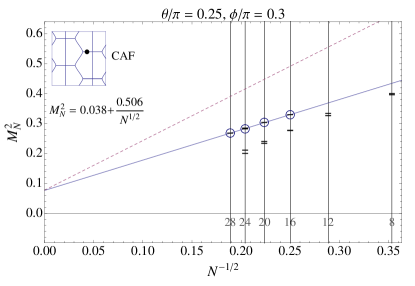
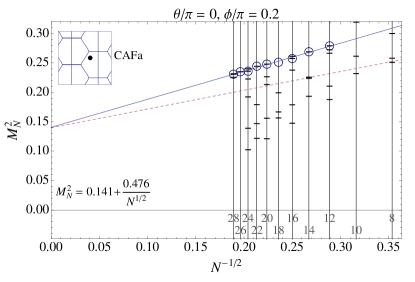
Figure 9: Finite-size scaling of the ordered moment in the columnar phase with antiferromagnetic $J_{2}$. Top: isotropic model, $J_{1a}=J_{1b}$. Bottom: maximally anisotropic case, $J_{1b}=0$. The horizontal dashes denote $M_{N}^{2}(\vec{Q})$ for different tilings, the solid lines are fits with Eq. (43) to the values for most-square-like-tiles, marked with a circle. Results for $\tilde{M}_{N}^{2}(\vec{Q})$ for individual tiles are not shown, fits to $\tilde{M}_{N}^{2}(\vec{Q})$ are displayed as the dashed lines. The extrapolated values obtained from the scaling correspond to half the value of the ordered moment, due to the spatial symmetry breaking introduced with columnar ordering.

Fig. 9 shows the scaling of the ordered moment in the columnar phase for antiferromagnetic $J_{2}$. For the isotropic case (top), as before only those tiles compatible with both columnar phases, equivalent to compatibility with all four classical phases can be used. In the infinite system, which has ${\cal C}_{4v}$ point-group symmetry, the wave vectors $(\pi,0)$ and $(0,\pi)$ are equivalent. However, most finite tiles have a spatial symmetry lower than ${\cal C}_{4}$ (see Table 1), meaning that the equivalence between $(\pi,0)$ and $(0,\pi)$ is lost. For this reason we take the sum of the structure factor at these two wave vectors and use the resulting data points for scaling. This is not necessary for the anisotropic case ($\theta\neq\pi/4,-3\pi/4$), of which an example is shown at the bottom of Fig. 9, since then CAFa and CAFb are different phases anyway. Here also a larger number of clusters is available for the scaling. Note that in Fig. 9 we plot the area dependence of the structure factor and the long-distance correlation function including the factor $\zeta(\vec{Q})=2$ introduced in Eq. (25), which is due to the spatial symmetry breaking induced by the columnar order.

IV.2.3 Magnetically disordered regimes

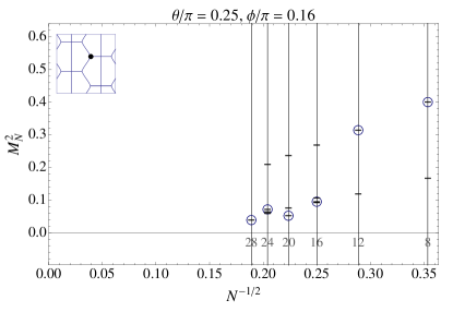
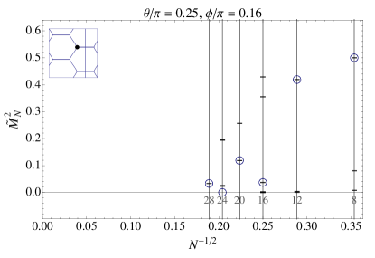
Figure 10: Tile area dependence of the ordered moment in the disordered regime at the NAF-CAF border for isotropic nearest-neighbor exchange. The values are obtained from (top) the structure factor and (bottom) the long-distance correlation function, and the circles show the values for the tiles with maximum squareness. No finite-size scaling is possible.

As it has been the case for the ground-state energy, in the disordered region between the Néel and the columnar phase of the isotropic model ($J_{1a}=J_{1b}=J_{1}$, $J_{2}/J_{1}\approx 1/2$), the behavior of both the structure factor and the correlation function do not show a systematic dependence on the tile size. This is obvious from Fig. 10, which shows the calculated values for both $M_{N}^{2}(\vec{Q})$ (top part) and $\tilde{M}_{N}^{2}(\vec{Q})$ (bottom part). Disregarding for once the squareness of our tiles, it appears that there are two “stripes” of values as a function of $1/\sqrt{N}$ which both seem to extrapolate roughly to $0$. However, a quantitative analysis in the sense of Eq. (43) cannot be made.

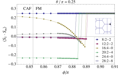
Figure 11: Dependence of the long-distance correlation function on the frustration angle $\phi$ in the spin nematic region between the CAF and FM phases of the isotropic model for those tiles with maximum squareness which are compatible to all four classical phases. The legend in the plot lists the individual tiles and their symbols.

We observe a very similar behavior also for $J_{2}/J_{1}\approx-1/2$ (with ferromagnetic $J_{1}$) in the spin-nematic region of the phase diagram. In order to see more details, the long-distance correlation function $\langle\vec{S}_{1}\vec{S}_{m}\rangle$, used in Eq. (38), in this narrow region between CAF and FM phase is plotted as a function of the frustration angle $\phi$ in Fig. 11 for tiles of different size. The labels of the individual tiles are given in the legend of the plot. The solid vertical line indicates the classical phase boundary. Apart from the eight-site tile, which is too small anyway because sites $1$ and $m$ are just two hops apart, for each tile $\langle\vec{S}_{1}\vec{S}_{m}\rangle$ is monotonously decreasing before jumping to the ferromagnetic value $\langle\vec{S}_{1}\vec{S}_{m}\rangle=S^{2}=1/4$. Those correlation functions which are ferromagnetic (positive, both sites $1$ and $m$ on the same sublattice) in the columnar phase even change their sign before the jump. This sign change possibly can serve as an indicator of the breakdown of columnar order. However, the transition to ferromagnetic correlations in the region of $0.881\pi<\phi<0.891\pi$ seen here is not happening uniformly for all tiles, hence it cannot be used to extrapolate to the thermodynamic limit. This will be discussed more quantitatively in the next section.

We can draw the same conclusions for the ordered moment scaling as we did before for the ground state energy: If we carefully select the allowed clusters with appropriate classical phase compatibility and maximum squareness we can carry out a well defined scaling procedure to the thermodynamic limit for the stable NAF and CAFa,b regions. However in the disordered regions at the borders of the CAFa/b honeycomb (see Fig. 1) scaling is impossible, which is an indication of the imminent breakdown of magnetic order due to quantum fluctuations. Similar conclusions were obtained already from linear spin wave theory Schmidt et al. (2010).

IV.3 Accuracy of extrapolated values

For the linear scaling (Eqs. (42) and (43) without the last term) applied to extrapolating the results to the infinite lattice, an analysis of the quality of the scaling is essential. There are several measures that can be introduced to characterize the quality of the scaling. A convenient measure is the relative error in the $\infty$-norm, generally defined as

$$\epsilon_{\text{rel}} = \frac{{\|f-d\|}_{\infty}}{{\|f\|}_{\infty}}\approx 10^{-p},$$ (44)

$$\|\{x_{1},x_{2},\dots\}\|_{\infty} = \max\left(|x_{1}|,|x_{2}|,\dots\right).$$

Here, $f$ is the set of fitted values at the points $1/N$, and $d$ the set of data calculated for the maximum-squareness tiles with area $N$. The exponent $p$ in the above equation can be interpreted as the number of significant digits Golub and Loan (1996) for the extrapolated value $f_{0}$ at $N\to\infty$.

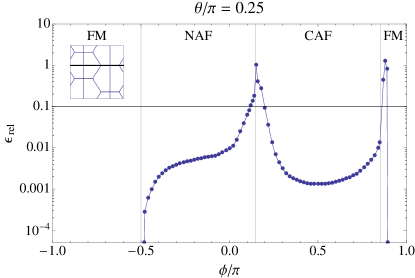
Figure 12: Relative error $\epsilon_{\text{rel}}$ as defined in Eq. (44) of the fits to $M_{N}^{2}(\vec{Q})$ for the isotropic model. Note the logarithmic scale of the ordinate. The error in the magnetically disordered regions is at least one order of magnitude larger than in the ordered sectors of the phase diagram. The solid horizontal line denotes the value $\epsilon_{\text{rel}}=0.1$, indicating the maximum error acceptable for having at least one significant digit in $M^{2}(\vec{Q})$.

Figure 12 shows a plot of $\epsilon_{\text{rel}}$ for $M_{N}^{2}(\vec{Q})$ of the isotropic model as function of the frustration angle $\phi$. In the ferromagnetic phase, the fully polarized state is the ground-state and the error reflects the numerical noise, i. e., the accuracy of the floating point operations, which are of order $10^{-15}$, and has been excluded from the figure. (We have determined $M_{N}^{2}(\vec{Q})$ for $(\phi,\theta)$ values in the ferromagnetic region mainly in order to verify the correctness of our numerical implementation of Eq. (43).)

In the well-ordered region of NAF and CAF we have $\epsilon_{\text{rel}}={\cal O}(10^{-3}\dots 10^{-2})$, and we can regard the scaling procedure in these areas as stable. This is in contrast to the magnetically disordered regions at the borders of the columnar phases, where the strong increase in $\epsilon_{\text{rel}}$ clearly indicates that the scatter of the points is much higher and makes the extrapolated value unreliable. The solid horizonal line in Fig. 12 denotes $\epsilon_{\text{rel}}=0.1$. According to Eq. (44), this is the maximum error at which the extrapolated values for $M^{2}(\vec{Q})$ have at least one significant digit. In other words, a magnetic order parameter $M^{2}(\vec{Q})$ to be used to characterize the nature of the ground state cannot be obtained anymore in those regions with $\epsilon_{\text{rel}}>0.1$.

V Results

Here we describe the systematic dependence of the thermodynamic limit of the ground state energy $E_{0}$ and the ordered moment $M_{0}(\vec{Q})$ on the model parameters $(\phi,\theta)$ as obtained from our finite-size analysis discussed in the previous section.

V.1 Ground-state energy

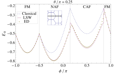
Figure 13: The ground-state energy as function of the frustration angle $\phi$ for the isotropic model with fixed $\theta=\pi/4$ . The classical energy is shown as dashed line, and the spin-wave results including zero-point fluctuations are presented as solid line. Dots indicate the values for the energy $E_{0}$ obtained from extrapolating our exact-diagonalization data.

Fig. 13 shows the energy dependence on the frustration angle $\phi$ for the isotropic model with $\theta/\pi=1/4$. The dashed line shows the classical energy, the solid line displays the result from linear spin wave theory which includes corrections due to zero-point fluctuations of magnons Schmidt et al. (2010). The dots denote our scaled ED results $E_{0}=E_{0}(\phi,\theta)$ according to Eq. (42).

Inside the magnetic phases, the overall agreement between the numerical data and the results obtained from linear spin-wave calculations Schmidt et al. (2010) (solid line) is surprisingly good, and improves on the comparison with exact diagonalization results from just a single cluster we have made previously Schmidt et al. (2010). However, in the disordered regions at the borders of the columnar phase, which is shaded with gray, the fit to the numerical data has a comparatively poor quality, and the reliability of the numerical result is somewhat questionable. Linear spin-wave theory breaks down here, too, albeit in a slightly different parameter range Schmidt et al. (2010).

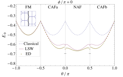
Figure 14: Ground state energy for the anisotropic model with first neighbor interaction only ($J_{2}=0$), as function of the anisotropy parameter $\theta$. The dashed line represents the energy of the classical model, the solid line includes corrections from linear spin wave theory. The extrapolated values from finite-size scaling of the ED results are shown as dots. Dashes denote the result $E_{0}=J_{\text{c}}\mathop{\rm ln}2$ from Bethe ansatz calculations for the one-dimensional $S=1/2$ spin chain.

Next we turn to the unfrustrated ($J_{2}=0$) but anisotropic ($J_{1a}\neq J_{1b}$) model with only next-nearest neighbor interactions. Fig. 14 shows the dependence of the ground-state energy per site $E_{0}$ on the anisotropy parameter $\theta$ for fixed frustration angle $\phi=0$. The classical ground-state energy is shown as a dashed line for comparison. As before, the agreement with linear spin-wave theory (solid line) inside the magnetic phases is good, which is not the case at the borders of the Néel phase.

But in this case, this has a reason different from the frustration induced by competing interactions discussed before: For $\theta=0$ or $\theta=\pi/2$, the nearest-neighbor exchange along one particular spatial direction vanishes, $J_{1a}$ or $J_{1b}$, respectively, such that we are actually dealing with an array of decoupled spin chains instead of a two-dimensional system. The classical approximation fails to describe the ground-state of the chains completely, and LSW corrections to it due to zero-point fluctuations are largest at these two points, improving the classical result drastically. The extrapolated ground-state energy from ED gives an even better approximation to the true value for $E_{0}=J_{\text{c}}\mathop{\rm ln}2$ derived from Bethe ansatz results Hulthén (1938), displayed as short horizontal dashes in Fig. 14, but also here the agreement is limited. However this is an extreme case, and we discuss it here primarily to show the limits of the finite-size scaling method when applied to the strongly anisotropic model.

V.2 Structure factor and ordered moment

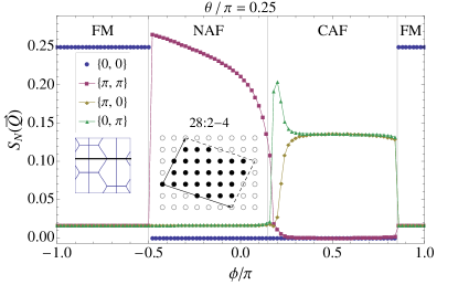
Figure 15: Structure factor $S_{N}(\vec{Q})$ for tile 28:2-4 (inset: illustration of the compact tile) at the wave vectors corresponding to the four classically ordered phases as a function of the frustration angle $\phi$ for the isotropic model. The labeling is explained in the inset of the figure.

The calculated values for the structure factor for all four ordering wave vectors as obtained using the Eq. (III.7), for the largest system we are considering (tile 28:2-4 with 28 spins) is shown in Fig. 15. Starting from the FM phase with a fully polarized ground state, we have $S_{N}(\vec{Q}_{\text{FM}})=S^{2}$, and at the antiferromagnetic wave vectors $\vec{Q}$ we get $S_{N}(\vec{Q})=1/60$ in accordance with Eq. (33).

Since the shape of tile 28:2-4 is a parallelogram, and hence has ${\cal C}_{2}$ point-group symmetry only, the equivalence between the two wave vectors $\vec{Q}=(\pi,0)$ and $(0,\pi)$ present for the infinite system (or any tile having at least ${\cal C}_{4}$ point-group symmetry) is lost. This manifests itself in a different $\phi$ dependence of the two structure factors $S(\vec{Q}_{\text{CAFa}})\neq S(\vec{Q}_{\text{CAFb}})$ in the columnar phase, see Fig. 15.

Moreover, the discontinuity between the value of the structure factor at the $(0,0)$ ordering in the FM phase and the $(\pi,\pi)$ ordering in the NAF phase ($\phi\approx-\pi/2$) is a finite-size effect and will be suppressed by increasing the cluster size.

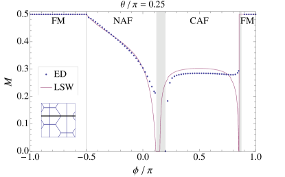
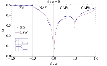
Figure 16: The extrapolated ordered moment as function of the frustration angle, for (top) the isotropic $\theta=\pi/4$ case and (bottom) the maximally anisotropic case with $\theta=0$. Those tiles with the maximum squareness are used for the scaling. The gray-shaded areas in the top plot represent the range of frustration angles $\phi$ where the relative error of $M^{2}(\vec{Q})$ is above $0.1$.

In Fig. 16 the extrapolated values for the ordered moment $M^{2}(\vec{Q})$ are plotted (with dots) as a function of the frustration angle $\phi$ at two different anisotropy parameters. The top (bottom) plot corresponds to the isotropic (maximally anisotropic) case. Again the overall agreement with linear spin-wave theory (solid lines in Fig. 16) is very good inside the ordered regimes of the phase diagram, and there are differences around the borders of the columnar phases. The gray-shaded areas in the upper plot denote the range of frustration angles $\phi$ with a relative error $\epsilon_{\text{rel}}>0.1$ (see Eq. (44)), indicating that in the magnetically disordered regions the numerical results tend to become unreliable.

In the spin-nematic region of the isotropic model, a qualitative difference exists between linear spin wave theory and exact diagonalization: With increasing $\phi$, the former yields a tiny region around the classical CAF/FM phase boundary where the ordered moment vanishes before jumping to saturation in the FM phase. In contrast, the extrapolated values for $M(\vec{Q})$ from our ED calculations remain finite at any frustration angle $\phi$.

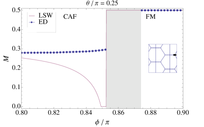
Figure 17: Ordered moment $M(\vec{Q})$ as a function of the frustration angle, for the isotropic $\theta=\pi/4$ case around the nematic region between columnar and FM phases. The solid line indicates the result from linear spin wave theory, the dots display the scaled ED values. The gray area shows the region where the relative error of the extrapolated value for $M^{2}(\vec{Q})$ is above 0.1.

This behavior is displayed with greater detail in Fig. 17, which shows $M(\vec{Q})$ as a function of $\phi$ around the classical phase boundary, both for linear spin-wave theory (solid line) and exact diagonalization (dots). The extrapolated moment shows a nearly constant $\phi$ dependence $M(\vec{Q}_{\text{CAFa}})\approx M^{\phi=0}(\vec{Q}_{\text{NAF}})$ in the columnar phase for $\phi/\pi\leq 0.855$, as it does in the FM phase with $M(\vec{Q}_{\text{FM}})=S$ for $\phi/\pi\geq 0.874$. However, for $0.855<\phi/\pi<0.874$, $M_{N}(\vec{Q})$ suddenly shows erratic behavior for different tile sizes (Fig. 11 shows this for the long-distance correlation function), correspondingly we have $\epsilon_{\text{rel}}>0.1$ (no significant digits for $M^{2}(\vec{Q})$) in that range of the frustration angle.

The point $\phi=0.874\pi$, where we can extrapolate $M_{N}(\vec{Q})$ to a stable limit (full polarization) again can be regarded as an upper bound of the border between spin nematic and FM phase. According to Fig. 11, the minimum value for $\phi$ where we get a stable $M(\vec{Q})=S$ decreases as a function of tile size, disregarding the smallest eight-site tile. However the true order parameter for the spin nematic phase is not of magnetic type, and therefore the behavior of $M(\vec{Q})$ cannot be used to understand the properties of this phase, in particular the parameter range within which it exists. Instead, one would have to calculate the spin nematic order parameter Shannon et al. (2006) in a similar way, which is beyond the scope of the present paper.

Finally, the dependence of the ordered moment on the anisotropy angle $\theta$ for the unfrustrated case with only nearest neighbor interaction ($\phi=0$, equivalent to $J_{2}=0$) is shown in Fig. 18. The dots display the ED extrapolation, the solid line shows the linear spin wave result. At the values $\theta=\pi/4$ and $\theta=-3/4\pi$, the isotropic model is recovered with the well-known values $M(\vec{Q}_{\text{NAF}})\approx 0.3$ and $M(\vec{Q}_{\text{FM}})=S=1/2$. We point out again that the points $\theta=0$ and $\theta=\pi/2$ at the borders of the Néel phase correspond to arrays of independent chains. Therefore the moment suppression at these points is not a frustration effect but a result of the effective one-dimensional character of the model, where no magnetic moment exists at any wave vector.

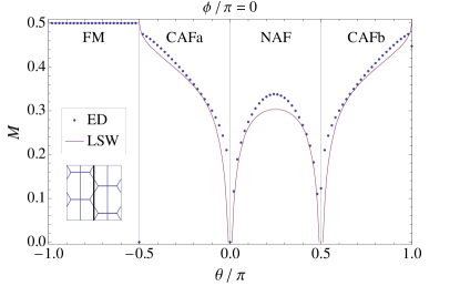
Figure 18: Ordered moment $M(\vec{Q})$ for fixed frustration angle $\phi=0$, equivalent to $J_{2}=0$, i. e., vanishing next-nearest neighbor exchange. Control parameter here is the anisotropy angle $\theta$; the points $\theta=\pi/4$ and $\theta=-3/4\pi$ denote the isotropic case. The solid line denotes the result from linear spin-wave theory, the dots display the values extrapolated from our ED calculations.

VI Summary

In this work we have investigated the anisotropic frustrated square lattice Heisenberg model using the exact diagonalization method for finite clusters applying a finite size scaling procedure. The latter is essential to obtain reliable values of ground state energy and ordered moment size in the thermodynamic limit. We have also compared the numerical results with those of linear spin wave theory Schmidt et al. (2010). The model which we have considered is characterized by an anisotropy parameter $\theta$ for the nearest neighbor interaction and a frustration angle $\phi$ characterizing the ratio of next nearest and nearest neighbor exchange.

The implementation of a stable finite size scaling procedure requires precise criteria for the usefulness of the many possible clusters of varying size and shape used to tile the lattice. We have introduced and described in great detail how all possible tilings with a given area $N$ of the square or rectangular lattice can be generated. Then we have classified the clusters according to their spatial symmetry, compatibility with classical magnetic phases and their geometrical compactness or squareness. We have found that a restriction to tiles which have compatibility with classical phases and maximal squareness lead to a very stable scaling behavior of ground state energy and ordered moment in the region of NAF and CAF phases. Close to the classical NAF/CAF and CAF/FM boundaries shown in Fig. 1 the relative error of energy and moment increases and the scaling procedure becomes unstable, because a systematic dependence of $E_{0N}$ and $M_{N}(\vec{Q})$ on the tile area $N$ ceases to exist. In these regions, a quantitative prediction of the size of the ordered moment becomes difficult, if not impossible. The frustration effects of competing exchange interactions lead to large quantum fluctuations which in turn cause the breakdown of magnetic order.

Using the scaling results we were able to calculate the systematic dependence of ground state energy and ordered moment as function of frustration and anisotropy angles $\phi$ and $\theta$ respectively. We found that in the columnar phases, introducing a spatial anisotropy strongly stabilizes the ordered moment. In fact it becomes larger than that of the conventional unfrustrated isotropic nearest neighbor NAF with $M(\vec{Q})\approx 0.3$. This stabilization effect becomes particularly pronounced in the CAF/FM transition region where the spin nematic phase of the isotropic model has been found.

The agreement of exact diagonalization results with spin wave calculations was found to be generally good. Both methods predict the breakdown of magnetic order in the transition regions at the borders of the columnar magnetic phases as function of frustration but also in the regions where the model attains effective quasi-one-dimensional character as function of the anisotropy for $J_{2}=0$. As in earlier investigations for the isotropic model, it remains difficult to quantify the exact size of the interval on the $\phi$ or $\theta$ axes where the ordered moment vanishes. Although not discussed here, the present work also has given a clear framework in which the field dependence of the ordered moment may be discussed.

Appendix A All distinct eight-site tilings of the square lattice

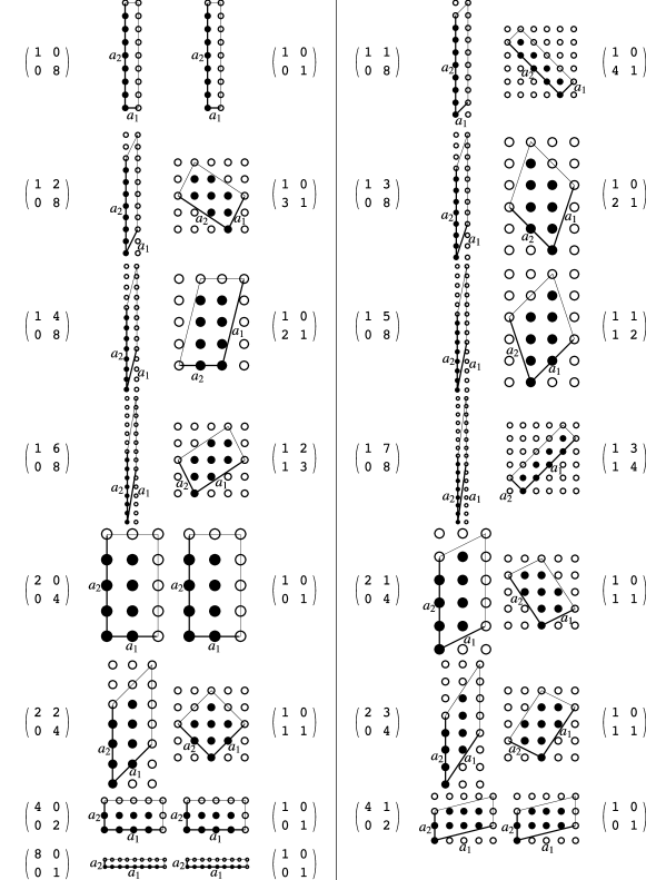
Figure 19: All 15 possible distinct square lattice tilings $\Lambda_{H}$ for a given tile size $N=8$. The columns display the HNF matrix $H$, a graphical sketch of the HNF tile, a graphical sketch of the corresponding compact tile, and the unimodular matrix $U^{-1}$ mapping $H$ onto $M_{\text{c}}$.

To demonstrate how to find all possible tilings with a given area $N$ of the square lattice, Fig. 19 displays a list of all the distinct lattice tilings for two-dimensional tiles of size $N=8$ created applying Eqs. (3) and (4). In each row, the HNF matrix $H$ is shown together with the HNF tile ${\cal T}_{H}$, the compact tile ${\cal T}_{M_{\text{c}}}$, and the unimodular matrix $U^{-1}$ needed to map $H$ onto $M_{\text{c}}$. Note that in order to discuss orthorhombic or trigonal symmetry breaking of the Hamiltonian, we do not regard tiles as identical which are related by a point-group operation on the square lattice.

References

- Melzi et al. (2000) R. Melzi, P. Carretta, A. Lascialfari, M. Mambrini, M. Troyer, P. Millet, and F. Mila, Phys. Rev. Lett., 85, 1318 (2000).
- Melzi et al. (2001) R. Melzi, S. Aldrovandi, F. Tedoldi, P. Carretta, P. Millet, and F. Mila, Phys. Rev. B, 64, 024409 (2001).
- Kaul et al. (2004) E. E. Kaul, H. Rosner, N. Shannon, R. V. Shpanchenko, and C. Geibel, J. Magn. Magn. Mat., 272-276, 922 (2004).
- Kaul (2005) E. Kaul, Experimental Investigation of new Low-Dimensional Spin Systems in Vanadium Oxides, Ph.D. thesis, Technische Universität Dresden, Dresden (2005).
- Kini et al. (2006) N. S. Kini, E. E. Kaul, and C. Geibel, J. Phys.: Cond. Mat., 18, 1303 (2006).
- Tsirlin and Rosner (2009) A. A. Tsirlin and H. Rosner, Phys. Rev. B, 79, 214417 (2009).
- Tsirlin et al. (2009) A. A. Tsirlin, B. Schmidt, Y. Skourski, R. Nath, C. Geibel, and H. Rosner, Phys. Rev. B, 80, 132407 (2009).
- Bombardi et al. (2004) A. Bombardi, J. Rodriguez-Carvajal, S. Di Matteo, F. de Bergevin, L. Paolasini, P. Carretta, P. Millet, and R. Caciuffo, Phys. Rev. Lett., 93, 027202 (2004).
- Skoulatos et al. (2007) M. Skoulatos, J. P. Goff, N. Shannon, E. E. Kaul, C. Geibel, A. P. Murani, M. Enderle, and A. R. Wildes, J. Magn. Magn. Mat., 310, 1257 (2007).
- Skoulatos et al. (2009) M. Skoulatos, J. P. Goff, C. Geibel, E. E. Kaul, R. Nath, N. Shannon, B. Schmidt, A. P. Murani, P. P. Deen, M. Enderle, and A. R. Wildes, Europhys. Lett., 88, 57005 (2009).
- Misguich et al. (2003) G. Misguich, B. Bernu, and L. Pierre, Phys. Rev. B, 68, 113409 (2003).
- Shannon et al. (2004) N. Shannon, B. Schmidt, K. Penc, and P. Thalmeier, Eur. Phys. J. B, 38, 599 (2004).
- Shannon et al. (2006) N. Shannon, T. Momoi, and P. Sindzingre, Phys. Rev. Lett., 96, 027213 (2006).
- Schmidt et al. (2007) B. Schmidt, P. Thalmeier, and N. Shannon, Phys. Rev. B, 76, 125113 (2007).
- Thalmeier et al. (2008) P. Thalmeier, M. E. Zhitomirsky, B. Schmidt, and N. Shannon, Phys. Rev. B, 77, 104441 (2008).
- Dagotto and Moreo (1989) E. Dagotto and A. Moreo, Phys. Rev. B, 39, 4744 (1989).
- Singh and Narayanan (1990) R. R. P. Singh and R. Narayanan, Phys. Rev. Lett., 65, 1072 (1990).
- Schulz and Ziman (1992) H. J. Schulz and T. A. L. Ziman, Europhys. Lett., 18, 355 (1992).
- Richter (1993) J. Richter, Phys. Rev. B, 47, 5794 (1993).
- Einarsson and Schulz (1995) T. Einarsson and H. J. Schulz, Phys. Rev. B, 51, 6151 (1995).
- Schulz et al. (1996) H. J. Schulz, T. A. L. Ziman, and D. Poilblanc, J. Phys. I France, 6, 675 (1996).
- Zhitomirsky et al. (2000) M. E. Zhitomirsky, A. Honecker, and O. A. Petrenko, Phys. Rev. Lett., 85, 3269 (2000).
- Honecker (2001) A. Honecker, Can. J. Phys., 79, 1557 (2001).
- Schmidt et al. (2010) B. Schmidt, M. Siahatgar, and P. Thalmeier, Phys. Rev. B, 81, 165101 (2010).
- Ceccatto et al. (1992) H. A. Ceccatto, C. J. Gazza, and A. E. Trumper, Phys. Rev. B, 45, 7832 (1992).
- Dotsenko and Sushkov (1994) A. V. Dotsenko and O. P. Sushkov, Phys. Rev. B, 50, 13821 (1994).
- Uhrig et al. (2009) G. S. Uhrig, M. Holt, J. Oitmaa, O. P. Sushkov, and R. R. P. Singh, Phys. Rev. B, 79, 092416 (2009).
- Gelfand et al. (1989) M. P. Gelfand, R. R. P. Singh, and D. A. Huse, Phys. Rev. B, 40, 10801 (1989).
- Oitmaa and Zheng (1996) J. Oitmaa and W. Zheng, Phys. Rev. B, 54, 3022 (1996).
- Oitmaa et al. (2006) J. Oitmaa, C. Hamer, and W. Zheng, Series Expansion Methods (Cambridge University Press, 2006).
- Read and Sachdev (1991) N. Read and S. Sachdev, Phys. Rev. Lett., 66, 1773 (1991).
- Sachdev and Read (1997) S. Sachdev and N. Read, Int. J. Mod. Phys. B, 5, 219 (1997).
- Singh et al. (1999) R. R. P. Singh, W. Zheng, C. J. Hamer, and J. Oitmaa, Phys. Rev. B, 60, 7278 (1999).
- Capriotti et al. (2001) L. Capriotti, F. Becca, A. Parola, and S. Sorella, Phys. Rev. Lett., 87, 097201 (2001).
- Capriotti et al. (2003) L. Capriotti, F. Becca, A. Parola, and S. Sorella, Phys. Rev. B, 67, 212402 (2003).
- Misguich and Lhuillier (2004) G. Misguich and C. Lhuillier, in Frustrated Spin Systems, edited by H. T. Diep (World Scientific, 2004).
- Sindzingre (2004) P. Sindzingre, Phys. Rev. B, 69, 094418 (2004).
- Bishop et al. (2008) R. F. Bishop, P. H. Y. Li, R. Darradi, and J. Richter, J. Phys.: Cond. Mat., 20, 255251 (2008).
- Moukouri (2004) S. Moukouri, Phys. Rev. B, 70, 014403 (2004).
- Ewings et al. (2008) R. A. Ewings, T. G. Perring, R. I. Bewley, T. Guidi, M. J. Pitcher, D. R. Parker, S. J. Clarke, and A. T. Boothroyd, Phys. Rev. B, 78, 220501(R) (2008).
- McQueeney et al. (2008) R. J. McQueeney, S. O. Diallo, V. P. Antropov, G. D. Samolyuk, C. Broholm, N. Ni, S. Nandi, M. Yethiraj, J. L. Zarestky, J. J. Pulikkotil, A. Kreyssig, M. D. Lumsden, B. N. Harmon, P. C. Canfield, and A. I. Goldman, Phys. Rev. Lett., 101, 227205 (2008).
- Diallo et al. (2009) S. O. Diallo, V. P. Antropov, T. G. Perring, C. Broholm, J. J. Pulikkotil, N. Ni, S. L. Bud’ko, P. C. Canfield, A. Kreyssig, A. I. Goldman, and R. J. McQueeney, Phys. Rev. Lett., 102, 187206 (2009).
- Zhao et al. (2009) J. Zhao, D. T. Adroja, D.-X. Yao, R. Bewley, S. Li, X. F. Wang, G. Wu, X. H. Chen, J. Hu, and P. Dai, Nat. Phys., 5, 555 (2009).
- Haan et al. (1992) O. Haan, J. U. Klaetke, and K. H. Mütter, Phys. Rev. B, 46, 5723 (1992).
- Betts et al. (1999) D. Betts, H. Lin, and J. Flynn, Can. J. Phys., 77, 353 (1999).
- Hasenfratz and Niedermayer (1993) P. Hasenfratz and F. Niedermayer, Z. Phys. B, 92, 91 (1993).
- Schrijver (1986) A. Schrijver, Theory of Linear and Integer Programming (John Wiley & Sons, Chichester, 1986).
- Domich et al. (1987) P. Domich, R. Kannan, and L. Trotter, Jr., Math. Oper. Res., 12, 50 (1987).
- Lyness et al. (1991) J. N. Lyness, T. Sørevik, and P. Keast, Math. Comp., 56, 243 (1991).
- Stewart et al. (1997) G. E. Stewart, D. D. Betts, and J. S. Flynn, J. Phys. Soc. Jpn., 66, 3231 (1997).
- Bernu et al. (1994) B. Bernu, P. Lecheminant, C. Lhuillier, and L. Pierre, Phys. Rev. B, 50, 10048 (1994).
- Sandvik (1997) A. W. Sandvik, Phys. Rev. B, 56, 11678 (1997).
- Note (1) For odd , tiles with squareness have four equivalent points with maximum distance from the origin.
- Golub and Loan (1996) G. Golub and C. Loan, Matrix Computations, Johns Hopkins studies in the mathematical sciences (Johns Hopkins University Press, 1996).
- Hulthén (1938) L. Hulthén, Arkiv för Matematik, Astronomi och Fysik, 26A, 1 (1938).