Liquid chromatography mass spectrometry-based proteomics: Biological and technological aspects

Abstract

Mass spectrometry-based proteomics has become the tool of choice for identifying and quantifying the proteome of an organism. Though recent years have seen a tremendous improvement in instrument performance and the computational tools used, significant challenges remain, and there are many opportunities for statisticians to make important contributions. In the most widely used “bottom-up” approach to proteomics, complex mixtures of proteins are first subjected to enzymatic cleavage, the resulting peptide products are separated based on chemical or physical properties and analyzed using a mass spectrometer. The two fundamental challenges in the analysis of bottom-up MS-based proteomics are as follows: (1) Identifying the proteins that are present in a sample, and (2) Quantifying the abundance levels of the identified proteins. Both of these challenges require knowledge of the biological and technological context that gives rise to observed data, as well as the application of sound statistical principles for estimation and inference. We present an overview of bottom-up proteomics and outline the key statistical issues that arise in protein identification and quantification.

T1Portions of this work were supported by the NIH R25-CA-90301 training grant in biostatistics and bioinformatics at TAMU, the National Institute of Allergy and Infectious Disease NIH/DHHS through interagency agreement Y1-AI-4894-01, National Center for Research Resources (NCRR) grant RR 18522, and were performed in the Environmental Molecular Science Laboratory, a United States Department of Energy (DOE) national scientific user facility at Pacific Northwest National Laboratory (PNNL) in Richland, WA. PNNL is operated for the DOE Battelle Memorial Institute under contract DE-AC05-76RLO01830.

, , , and

1 Introduction

The 1990s marked the emergence of genome sequencing and deoxyribonucleic acid (DNA) microarray technologies, giving rise to the “-omics” era of research. Proteomics is the logical continuation of the widely-used transcriptional profiling methodology [Wilkins et al. (1996)]. Proteomics involves the study of multiprotein systems in an organism, the complete protein complement of its genome, with the aim of understanding distinct proteins and their roles as a part of a larger networked system. This is a vital component of modern systems biology approaches, where the goal is to characterize the system behavior rather than the behavior of a single component. Measuring messenger ribonucleic acid (mRNA) levels as in DNA microarrays alone does not necessarily tell us much about the levels of corresponding proteins in a cell and their regulatory behavior, since proteins are subjected to many post-translational modifications and other modifications by environmental agents. Proteins are responsible for the structure, energy production, communications, movements and division of all cells, and are thus extremely important to a comprehensive understanding of systems biology.

While genome-wide microarrays are ubiquitous, proteins do not share the same hybridization properties of nucleic acids. In particular, interrogating many proteins at the same time is difficult due to the need for having an antibody developed for each protein, as well as the different binding conditions optimal for the proteins to bind to their corresponding antibodies. Protein microarrays are thus not widely used for whole proteome screening. Two-dimensional gel electrophoresis (2-DE) can be used in differential expression studies by comparing staining patterns of different gels. Quantitation of proteins using 2-DE has been limited due to the lack of robust and reproducible methods for detecting, matching and quantifying spots as well as some physical properties of the gels [Ong and Mann (2005)]. Although efforts have been made to provide methods for spot detection and quantification [Morris, Clark and Gutstein (2008)], 2-DE is not currently the most widely-used technology for protein quantitation in complex mixtures. Meanwhile, mass spectrometry (MS) has proven effective for the characterization of proteins and for the analysis of complex protein samples [Nesvizhskii, Vitek and Aebersold (2007)]. Several MS methods for interrogating the proteome have been developed: Surface Enhanced Laser Desorption Ionization (SELDI) [Tang, Tornatore and Weinberger (2004)], Matrix Assisted Laser Desorption Ionization (MALDI) [Karas et al. (1987)] coupled with time-of-flight (TOF) or other instruments, and gas chromatography MS (GC-MS) or liquid chromatography MS (LC-MS). SELDI and MALDI do not incorporate online separation during MS analysis, thus, separation of complex mixtures needs to be performed beforehand. MALDI is widely used in tissue imaging [Caprioli, Farmer and Gile (1997); Cornett et al. (2007); Stoeckli et al. (2001)]. GS-MS or LC-MS allow for online separation of complex samples and thus are much more widely used in high-throughput quantitative proteomics. Here we focus on the most widely-used “bottom-up” approach to MS-based proteomics, LC-MS.

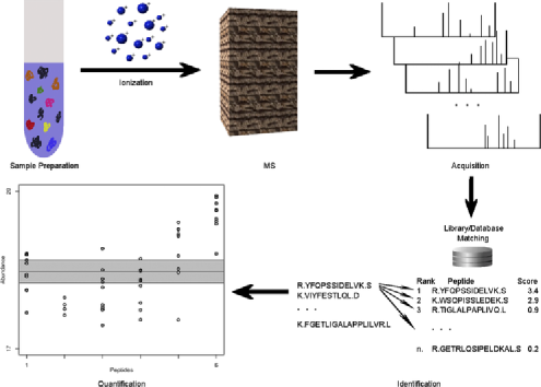
Figure 1: Overview of LC-MS-based proteomics. Proteins are extracted from biological samples, then digested and ionized prior to introduction to the mass spectrometer. Each MS scan results in a mass spectrum, measuring m/z values and peak intensities. Based on observed spectral information, database searching is typically employed to identify the peptides most likely responsible for high-abundance peaks. Finally, peptide information is rolled up to the protein level, and protein abundance is quantified using either peak intensities or spectral counts.

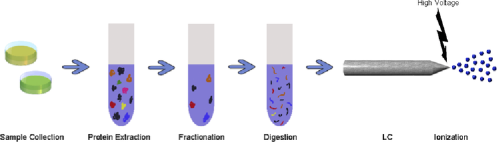
Figure 2: Sample preparation. Complex biological samples are first processed to extract proteins. Proteins are typically fractionated to eliminate high-abundance proteins or other proteins that are not of interest. The remaining proteins are then digested into peptides, which are commonly introduced to a liquid chromatography column for separation. Upon eluting from the LC column, peptides are ionized.

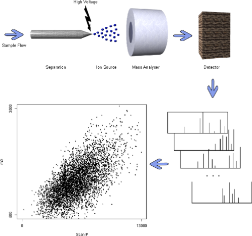
Figure 3: Mass spectrometry. The mass spectrometer consists of an ion source, responsible for ionizing peptides, the mass analyzer and the detector, responsible for recording m/z values and intensities, respectively, for each ion species. Each MS scan results in a mass spectrum, and a single sample may be subjected to thousands of scans.

In LC-MS-based proteomics, complex mixtures of proteins are first subjected to enzymatic cleavage, then the resulting peptide products are analyzed using a mass spectrometer; this is in contrast to “top-down” proteomics, which deals with intact proteins and is limited to simple protein mixtures [Han, Aslanian and Yates (2008)]. A standard bottom-up experiment has the following key steps (Figures 1–3): (a) extraction of proteins from a sample, (b) fractionation to remove contaminants and proteins that are not of interest, especially high abundance house-keeping proteins that are not usually indicative of the disease being studied, (c) digestion of proteins into peptides, (d) post-digestion separations to obtain a more homogeneous mixture of peptides, and (e) analysis by MS. The two fundamental challenges in the analysis of MS-based proteomics data are then the identification of the proteins present in a sample, and the quantification of the abundance levels of those proteins. There are a host of informatics tasks associated with each of these challenges (Figures 4–6).

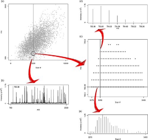
Figure 4: Data acquisition: (a) Scan numbers and m/z values for an example raw LC-MS data set. Each individual scan contains a single mass spectrum. (b) The mass spectrum for scan 5338. (c) A zoomed-in look at the scans 5275–5400 in m/z range 753–755.5. The cluster of dots is indicative of a single LC-MS “feature.” (d) The isotopic distribution for this feature in scan 5280. Peaks are separated by approximately $1/3$, indicating a charge state of $+3$. The monoisotopic mass is thus $753.36\times 3=2260.08$ Da. (e) The elution profile at m/z 753.36.

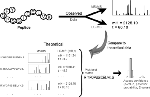
Figure 5: Protein identification. Peptide and protein identification is most commonly accomplished by matching observed spectral measurements to theoretical or previously-observed measurements in a database. In LC-MS/MS, measurements consist of fragmentation spectra, whereas mass and elution time alone are used in high-resolution LC-MS. Once a best match is found, one of the following methods for assessing confidence in the match is employed: decoy databases, empirical Bayes, or “expectation values.”

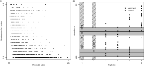
Figure 6: Protein quantitation. The left panel shows the proportion of missing values in an example data set as a function of the mean of the observed intensities for each peptide. There is a strong inverse relationship between these, suggesting that many missing intensities have been censored. The right panel shows an example protein found to be differentially expressed in a two-class human study. The protein had 6 peptides that were identified, although two were filtered out due to too many missing values (peptides 1 and 2, as indicated by the vertical shaded lines). Estimated protein abundances and confidence intervals are constructed from the peptide-level intensities by a censored likelihood model [Karpievitch et al. (2009a)].

The first step in protein identification is the identification of the constituent peptides. This is carried out by comparing observed features to entries in a database of theoretical or previously identified peptides (Figure 5). In tandem mass spectrometry (denoted by MS/MS), a parent ion possibly corresponding to a peptide is selected in MS¹ for further fragmentation in MS². Resulting fragmentation spectra are compared to fragmentation spectra in a database, using software like SEQUEST [Eng, McCormack and Yates (1994)], Mascot [Perkins et al. (1999)] or X!Tandem Alternatively, high-resolution MS instruments can be used to obtain extremely accurate mass measurements, and these can be compared to mass measurements in a database of peptides previously identified with high confidence via MS/MS [Pasa-Tolic et al. (2004)] using the same software tools above. In either case, a statistical assessment of the peptide identification confidence level is desired. Protein identification can be carried out by rolling up peptide-level identification confidence levels to the protein level, a process that is associated with a host of issues and complexities [Nesvizhskii et al. (2003)]. The goal of the identification process is generally to identify as many proteins as possible, while controlling the number of false identifications at a tolerable level. There are a myriad of options for the exact identification method used, including (i) the choice of a statistic for scoring the similarity between an observed spectral pattern and a database entry [Craig and Beavis (2004); Perkins et al. (1999)], and (ii) the choice of how to model the null distribution of the similarity metric [Elias and Gygi (2007); Keller et al. (2002)]. Two other methods of protein identification exist: de novo and hybrids of de novo and database matching. This is further explained in Section 5.

In quantitation experiments, protein abundances are inferred from the identified peptides. One of the most common and simplest methods is to count the number of times a peptide has been seen and accumulate those counts for all the peptides seen for a given protein. This gives a value that is proportional to the abundance of the protein, that is, a more abundant protein would be expected to have peptides that are observed more often [Liu, Sadygov and Yates (2004); Zhang et al. (2009)]. A more accurate method for quantifying the abundance of a peptide is to calculate the peak volume (or area) across its elution profile using its extracted ion chromatogram. Protein abundances are inferred from the corresponding peptide abundances (Figure 6). Peak capacity is a function of the number of ions detected for a particular peptide, and is related to peptide abundance [Old et al. (2005)]. Peptide abundances can be computed with or without the use of stable isotope labels [Gygi et al. (1999); Wang et al. (2003)]. In the case of isotopic labeled experiments, usually a ratio of the peak capacities of the two isotopically labeled components is reported. Regardless of the specific technology used to quantify peptide abundances, statistical models are required to roll peptide-level abundance estimates up to the protein level. Issues include widespread missing data due to low-abundance peptides, misidentified peptides, undersampling of peaks for fragmentation in MS/MS, and degenerate peptides that map to multiple proteins, among others. This is further explained in Section 6.

The purpose of this paper is to provide an accessible overview of LC-MS-based proteomics. Our template for this paper was a 2002 Biometrics paper of similar focus in the DNA microarray setting [Nguyen et al. (2002)]. It is our hope that this, like the 2002 paper for DNA microarrays, will serve as an entry-point for more statisticians to join the exciting research that is ongoing in the field of LC-MS-based proteomics.

2 Basic biological principles underlying proteomics

Proteins are the major structural and functional units of any cell. Proteins consist of amino acids arranged in a linear sequence, which is then folded to make a functional protein. The sequence of amino acids in proteins is encoded by genes stored in a DNA molecule. The transfer of information from genetic sequence to protein in eukaryotes proceeds by transcription and translation. In transcription, single-stranded mRNA representations of a gene are constructed. The mRNA leaves the nucleus and is processed into protein by the ribosome in the translation step. This information transfer, from DNA to mRNA to protein, is essential for cell viability and function. In genomic studies, microarray experiments measure gene expression levels by measuring the transcribed mRNA abundance. Such measurements can show the absence, under- or over-expression of genes under different conditions. However, protein levels do not always correspond to the mRNA levels due to a variety of factors such as alternative splicing or post translational modifications (PTMs). Thus, proteomics serves an important role in a systems-level understanding of biological systems.

A three-nucleotide sequence (codon) of mRNA encodes for one amino acid in a protein. The genetic code is said to be degenerate, as more than one codon can specify the same amino acid. In theory, mRNA could be read in three different reading frames producing distinct proteins. In practice, however, most mRNAs are read in one reading frame due to start and stop codon positions in the sequence. The raw polypeptide chain (a chain of amino acids constituting a protein) that emerges from the ribosome is not yet a functional protein, as it will need to fold into its 3-dimensional structure. In most organisms, proper protein folding is assisted by proteins called chaperones that stabilize the unfolded or partially folded proteins, preventing incorrect folding, as well as chaperonins that directly facilitate folding. Misfolded proteins are detected and either refolded or degraded. Proteins also undergo a variety of PTMs, such as phosphorilation, ubiquitination, methylation, acetylation, glycosylation, etc., which are additions/removals of specific chemical groups. PTMs can alter the function and activity level of a protein and play important roles in cellular regulation and response to disease or cellular damage.

A key challenge of proteomics is the high complexity of the proteome due to the one-to-many relationship between genes and proteins and the wide variety of PTMs. Furthermore, MS-based proteomics does not have the benefit of probe-directed assays like those used in microarrays. Although protein arrays are available, they (a) are challenging to design and implement and (b) are not well suited for protein discovery, and are thus not as widely used as MS-based technologies [Nesvizhskii, Vitek and Aebersold (2007)]. Several steps are involved in preparing samples for MS, such as protein extraction, fractionation, digestion, separation and ionization, and each contributes to the overall variation observed in proteomics data. In addition, technical factors like day-to-day and run-to-run variation in the complex experimental equipment can create systematic biases in the data-acquisition stage.

3 Experimental procedure

A LC-MS-based proteomic experiment requires several steps of sample preparation (Figure 2), including cell lysis to break cells apart, protein separation to spread out the collection of proteins into more homogenous groups, and protein digestion to break intact proteins into more manageable peptide components. Once this is complete, peptides are further separated, then ionized and introduced into the mass spectrometer.

3.1 Sample preparation

Analysis of the complete cell proteome usually involves collecting intact cells, washing them and adding a lysate buffer, containing a combination of chemicals that break the cell membrane and protease inhibitors that prevent protein degradation. Cells are homogenized and incubated with the buffer, after which centrifugation is used to separate the cellular debris and membrane from the supernatant, or cell lysate. The cell lysis step is unnecessary when analyzing bodily fluids such as blood serum. Blood samples are centrifuged, after which red blood cells pellet at the bottom of the tube, and plasma is collected at the top. Fibrinogen and other clotting factors are removed to obtain serum. High abundance proteins are also removed, as usually they do not play a role in disease. If some of the high abundance proteins are not removed, they may dominate spectral features and obscure less abundant proteins of interest. In LC-MS/MS, for example, the most abundant peptides are selected in the first MS step for further fragmentation in the following MS step, and only peptides selected for further fragmentation have a chance to be identified; see Section 3.2 for more details.

Because of the complexity of the proteome, separation steps are employed to spread out the proteins according to different chemical or physical characteristics, making it easier to observe a greater number of proteins in more detail. At the protein level, two-dimensional gel electrophoresis (2-DE) is often used to separate on the basis of both isoelectric point and mass [Berth et al. (2007); Gorg, Weiss and Dunn (2004)]. Proteins in the gel can be stained and extracted. Analyzing each stained region of the gel separately, for example, would allow for more detailed assessment of the total collection of proteins in the sample than if all proteins were analyzed at once. One of the main sources of error in the gel analysis is unequal precipitation of the proteins between gels. Thus, horizontal or vertical shifts and even diagonal stretching effects can be seen in two-dimensional (2-D) gels, necessitating alignment of all the gels to a reference gel. After gel alignment, spot detection is performed which may introduce further errors; see Section 7.2 for more details.

To facilitate protein identification, proteins are usually cleaved/digested chemically or enzymatically into fragments. Digestion overcomes many of the challenges associated with the complex structural characteristics of proteins, as the resulting peptide fragments are more tractable chemically, and their reduced size, compared to proteins, makes them more amenable to MS analysis. As examples of digestion agents, the trypsin enzyme cleaves at the carboxyl side of lysine and arginine residues, except when either is followed by proline, while chemical cyanogen bromide (CNBr) cleaves at the carboxyl site of methionine residues; trypsin is the most commonly used digestive enzyme. Specificity of the trypsin enzyme allows for the prediction of peptide fragments expected to be produced by the enzyme and create theoretical databases. Enzymatic digestion of proteins could be achieved in solution or gel, although digestion in solution is usually preferred, as gel is harder to separate from the sample after digestion. Missed cleavages can cause misidentified or missed peptides when searched against the database. Database searches can be adjusted to include one or more missed cleavages, but such searches take longer to complete.

Multiple distinct peptides can have very similar or identical molecular masses and thus produce a single intense peak in the initial MS (MS${}^{1})$ spectrum, making it difficult to identify the overlapping peptides. The use of separation techniques not only increases the overall dynamic range of measurements (i.e., the range of relative peptide abundances) but also greatly reduces the cases of coincident peptide masses simultaneously introduced into the mass spectrometer. We will describe one of the most commonly used separation techniques, high-performance liquid chromatography (HPLC), which is generally practiced in a capillary column format for proteomics. Other separation techniques exist and are similar in that they separate based on some molecular properties.

A HPLC system consists of a column packed with nonpolar (hydrophobic) beads, referred to as the stationary phase, a pump that creates pressure and moves the polar mobile phase through the column and a detector that captures the retention time. The sample is diluted in the aqueous solution and added to the mobile phase. As the peptides are pushed through the column, they bind to the beads proportionally to their hydrophobic segments. Thus, hydrophilic peptides will elute faster than hydrophobic peptides. HPLC separation allows for the introduction of only a small subset of peptides eluting from the LC column at a particular time into the mass spectrometer. Peptides of similar molecular mass but different hydrophobicity elute from the LC column and enter the mass spectrometer at different times, no longer overlapping in the initial MS analysis. The additional time required for the LC separation is well worth the effort, as the reduction in the overlap of the peptides of the same mass in MS¹ phase dramatically increases peak resolution (and hence, peak capacity). Note that LC columns must be regularly replaced, and it is common to observe systematic differences in the elution times of similar samples on difference columns. Thus, replacing a column during an experiment may contribute to technical variation in the resulting observed abundances between two columns.

Further separation techniques include sample fractionation prior to HPLC, and complementary techniques such as Ion Mobility Separation (IMS) after HPLC. Multidimensional LC has been successfully used to better separate peptides. Strong cation exchange (SCX) chromatography is usually used as a first separation step and reversed-phase chromatography (RPLC) as a secondary separation step because of its ability to remove salts and its compatibility with MS through electrospray ionization (ESI, described below) [Lee et al. (2006); Link et al. (1999); Peng et al. (2003); Sandra et al. (2009); Sandra et al. (2008)]. Combination of SCX with RPLC forms the basis of the Multidimensional Protein Identification Technology (MudPIT) approach [Washburn, Wolters and Yates (2001); Wolters, Washburn and Yates (2001)]. While multidimensional LC is capable of achieving greater separation, it requires larger sample quantities and more analysis time. In HPLC coupled with IMS, peptides eluting from the HPLC system are ionized using ESI, and the ions are injected into a drift tube containing neutral gas at controlled pressure. An electric field is applied, and the ions separate by colliding with the gas molecules. Larger ions experience more collisions with the gas and take longer to travel through the drift tube than smaller ions. IMS is very fast as compared with HPLC and, when used in conjunction with HPLC, achieves better separation than HPLC alone. IMS is not entirely orthogonal to HPLC, but it has been shown to increase the peak capacity (number of detected peaks) by an order of magnitude [Belov et al. (2007)]. While not currently in wide use, IMS technologies are rapidly evolving, and MS-based proteomics will likely involve multiple dimensions of separation based on both IMS and HPLC in the near future. New algorithms will need to be developed and existing ones modified to incorporate the extra separation dimensions.

3.2 Mass spectrometry

A mass spectrometer measures the mass-to-charge ratio (m/z) of ionized molecules. Recent years have seen a tremendous improvement in MS technology, and there are about 20 different mass spectrometers commercially available for proteomics. All mass spectrometers are designed to carry out the distinct functions of ionization and mass analysis. The key components of a mass spectrometer are the ion source, mass analyzer and ion detector (Figure 3). The ion source is responsible for assigning charge to each peptide. Mass analyzers take many different forms but ultimately measure the mass-to-charge (m/z) ratio of each ion. The detector captures the ions and measures the intensity of each ion species. In terms of a mass spectrum, the mass analyzer is responsible for the m/z information on the x-axis, and the detector is responsible for the peak intensity information on the y-axis.

Ionization methods include electron impact, chemical ionization, fast atom bombardment, field desorption, electrospray ionization (ESI) and laser desorption, and they usually operate by the addition of protons to the peptides. ESI and matrix assisted laser desorption/ionization (MALDI) are the most widely used methods in proteomics. In the ESI method, the sample is prepared in liquid form at atmospheric pressure and flows into a very fine needle that is subjected to a high voltage. Due to the electrostatic repulsion, the solvent drops leaving the needle tip dissociate to form a fine spray of highly charged droplets. As the solvent evaporates, the droplets disappear, leaving highly charged molecules. ESI is the most effective interface for LC-MS, as it naturally accommodates peptides in liquid solution. ESI is a soft ionization method, in that it achieves ionization without breaking chemical bonds and further fragmenting the peptides. In MALDI analysis, the biological molecules are dispersed in a crystalline matrix. A UV laser pulse is then directed at the matrix, which causes the ionized molecules to eject so that they can be extracted into a mass spectrometer.

The mass analyzer is key to the sensitivity, resolution and mass accuracy of an instrument. Sensitivity describes an instrument’s ability to detect low-abundance peptides, resolution to its ability to distinguish ions of very similar m/z values, and mass accuracy to its ability to obtain mass measurements that are very close to the truth. There are several basic mass analyzer types: quadrupole (Q), ion-trap (IT), time-of-flight (TOF), Fourier transform ion cyclotron resonance (FTICR), and the orbitrap. Different analyzers are commonly combined to achieve the best utilization as a single mass spectrometer (e.g., Q-TOF, triple-Q). We do not go into the details of the different mass analyzer types; interested readers are pointed elsewhere [Domon and Aebersold (2006); Siuzdak (2003)].

In tandem MS (referred to as MS/MS or MSⁿ), multiple rounds of MS are carried out on the same sample. This results in detailed signatures for detected features, which can be used for identification. Most MS/MS instruments can automatically select several of the most intense (high abundance) peaks from a parent MS (MS${}^{1})$ scan and subjects the corresponding ions (precursor or parent ions) for each to further fragmentation, followed by further scans. This process is repeated until all candidate peaks of a parent scan are exhausted [Domon and Aebersold (2006); Zhang et al. (2005)]. This results in a fragmentation pattern for each selected peptide, providing detailed information on the chemical makeup of the peptide. While the resulting fragmentation patterns are the basis for identification, MS/MS suffers from undersampling, in that relatively few (and generally only higher intensity) precursor ions are selected for fragmentation [Domon and Aebersold (2006); Garza and Moini (2006); Zhang et al. (2005)]. The issue of undersampling is not serious enough to steer away from using MSⁿ for protein identification and quantitation, but researchers should remember that not all peptides will have equal chances of being selected for fragmentation and thus may not be observed in the subsequent MS scans. Furthermore, MS/MS is time-intensive and thus not always ideal for high-throughput analysis [Masselon et al. (2008)]. Nevertheless, MS/MS is widely used for quantitative MS-based proteomics and forms the basis for most peptide and protein identification procedures (Section 5). Typically, MS/MS is preceded by LC separation and can more accurately be denoted by LC-MS/MS.

High-resolution LC-MS instruments (e.g., FTICR) are very fast and can achieve mass measurements that are sufficiently accurate for identification purposes. Furthermore, since fragmentation and repeated scans are not required, the undersampling issues due to peptide selection for MS/MS are avoided. Still, fragmentation patterns are valuable for identification, and so hybrid platforms involving both LC-MS/MS and high-resolution LC-MS are increasingly being used. One such example is the Accurate Mass and Time (AMT) tag approach [Pasa-Tolic et al. (2004); Tolmachev et al. (2008); Yanofsky et al. (2008)]. In the AMT tag approach, MS/MS analysis is used to create an AMT database of peptide theoretical mass and predicted elution time, based on high-confidence identifications from fragmentation patterns, followed by a single MS run on FTICR to obtain highly accurate mass measurements, as well as liquid chromatography elution times; peptide identification is then made by comparing the observed mass measurements and elution times to the AMT database entries. We note that an AMT database is typically constructed using many LC-MS/MS runs, resulting in a nearly complete database of proteotypic peptides [Mallick et al. (2007)]. Because in the AMT-based approach LC-MS spectra are matched to the database built from previous multiple MS/MS scans, the undersampling associated with LC-MS/MS on individual samples is avoided.

4 Data acquisition

In LC-MS, each sample may give rise to thousands of scans, each containing a mass spectrum [Figure 4(a)]. The mass spectrum for a single MS scan can be summarized by a plot of m/z values versus peak intensities [Figure 4(b)]. Buried in these data are signals that are specific to individual peptides. As a first step toward identifying and quantifying those peptides, features need to be identified in the data and, for example, distinguished from background noise. The first step in this is MS peak detection. Many approaches to peak detection have been proposed, as this is an old problem in the field of signal processing. Our lab employs a simple filter on the signal-to-noise ratio of a peak relative to its local background [Jaitly et al. (2009)]. Each peptide gives an envelope of peaks due to a peptide’s constituent amino acids. The presence of a peptide can be characterized by the m/z value corresponding to the peak arising from the most common isotope, referred to as the monoisotopic mass. While there are several isotopes of the elements that make up amino acids, ¹³C is the most abundant, constituting about 1.11% of all carbon species. Since the mass difference between ¹³C and ¹²C is approximately 1 Da, the monoisotopic peak for a peptide will be separated from an isotope with a single ¹³C by approximately $1/z$, where $z$ is the charge state of that peptide. Similarly, isotopes with additional copies of ¹³C will be separated in units of approximately $1/z$. [Figure 4(d)].

The process of deisotoping a spectrum is often used to simplify the data by removing the redundant information from isotopic peaks and involves (i) locating isotopic distributions in a MS scan, (ii) computing the charge state of each peptide based on the distance between the peaks in its isotopic distribution, and (iii) extracting each peptide’s monoisotopic mass. Note that this step is only possible if sufficiently high-resolution mass measurements have been obtained, as otherwise isotopic peaks can not be resolved. For (i), detected peaks are considered as possible members of an isotopic distribution, and theoretical isotopic distributions, derived from a database of peptide sequences, are overlaid with the observed spectra. A measure of fit is computed, and the peaks are called an isotopic distribution if the fit is good enough. One of the challenges encountered in deisotoping is the presence of overlapping isotopic distributions from different peptides. There are many algorithms available for peak detection and deisotoping, including commercial software from vendors such as Agilent, Rosetta Biosoftware and Thermo Fisher. Our lab uses Decon2LS [Jaitly et al. (2009)], open-source software that implements a variation of the THRASH algorithm [Horn, Zubarev and McLafferty (2000)]; the Decon2LS publication contains an extensive discussion of the above issues, as well as many helpful references for the interested reader.

A peptide will likely elute from the HPLC over multiple scans, creating an elution profile [Figure 4(e)]. Elution profiles for peptides are typically relatively short in duration, and serve to define a feature in LC-MS data sets. However, there are often contaminants present in an LC-MS sample with very long elution profiles, and these are filtered out in preprocessing steps. Various approaches to summarizing an elution profile are available. Our lab computes a normalized elution time (NET) [Petritis et al. (2006)]. At this stage, an LC-MS sample has been resolved into a list of LC-MS features, each with an assigned monoisotopic mass and an elution time. However, due to mass measurement errors and the random nature of elution times, (mass, elution time) assigned pairs will vary between LC-MS samples. Alignment is often performed to line up the LC-MS features in different samples. There are several algorithms for LC-MS alignment; examples include Crawdad [Finney et al. (2008)] and LCMSWarp [Jaitly et al. (2006)].

As with all high-throughput -omics technologies, MS-based proteomic data is typically subjected to substantial preprocessing and normalization. Systematic biases are often seen in mass measurements, elution times and peak intensities [Callister et al. (2006); Petyuk et al. (2008)]. Filtering of poor-quality proteins and peptides is also common [Karpievitch et al. (2009a)]. In normalization, care must be taken to separate biological signal from technical bias [Dabney and Storey (2006)]. Widely-used normalization techniques in high-throughput genomic or proteomic studies involve some variation of global scaling, scatterplot smoothing or ANOVA [Quackenbush (2002)]. Global scaling generally involves shifting all the measurements for a single sample by a constant amount, so that the means, medians or total ion currents (TICs) of all samples are equivalent. Since common technical biases are more complex than simple shifts between samples, global scaling is unable to capture complex bias features. Scatterplot smoothing, TIC and ANOVA normalization methods are sample-specific and hence more flexible. However, more complex preprocessing steps can result in overfitting, causing errors in downstream inference. For example, fitting a complex preprocessing model may use up substantial degrees of freedom, and analyzing the processed data, assuming that no degrees of freedom have been used, may result in overly optimistic accuracy levels and overestimated statistical significance; specific examples can be seen in Karpievitch et al. (2009b). Ideally, preprocessing would be carried out simultaneously with inference, or the downstream inferential steps would incorporate knowledge of what preprocessing was done [Leek and Storey (2007)]. A recently proposed method, called EigenMS, removes bias of arbitrary complexity by the use of the singular value decomposition to capture and remove biases from LC-MS peak intensity measurements [Karpievitch et al. (2009b)]. EigenMS removes biases of arbitrary complexity and adjusts the normalized intensities to correct the p-values after normalization (ensuring that null p-values are uniformly distributed).

Mass spectrometer manufacturers have developed a variety of proprietary binary data formats to store instrument output. Examples include .baf (Bruker), .Raw (Thermo) and .PKM (Applied Biosystems). Handling data in different proprietary formats typically requires corresponding proprietary software, making it difficult to share datasets. Several open-source, XML-based vendor-independent data formats have recently been developed to address this limitation: mzXML [Lin et al. (2005); Pedrioli et al. (2004)], mzData [Orchard et al. (2007)] and mzML [Deutsch (2008); Orchard et al. (2009)]. mzML 1.0 was released in June 2009 and is considered a merge of the best of mzData and mzXML. The format can store spectral information, instrument information, instrument settings and data processing details. mzML also has extensions such as chromatograms and multiple reaction monitoring (MRM) profile capture, and it now replaces both mzData and mzXML.

5 Protein identification

In bottom-up proteomics protein identification is usually accomplished by first comparing observed MS features to a database of predicted or previously identified features (e.g., by MS/MS or on the basis of previous analysis of a well characterized sample, Figure 5). The most widely-used approach is tandem MS with database searching [Nesvizhskii, Vitek and Aebersold (2007)], in which peptide fragmentation patterns are compared to theoretical patterns in a database using software like Sequest [Eng, McCormack and Yates (1994)], X!Tandem [Craig and Beavis (2004)] and Mascot [Perkins et al. (1999)]. With high-resolution LC-MS instruments, identifications can be made on the basis of mass and elution time alone, or in conjunction with MS/MS fragmentation patterns [Pasa-Tolic et al. (2004)]. Alternatives to database-searching include (i) de novo peptide sequencing [Dancik et al. (1999); Johnson et al. (2005); Lu and Chen (2003); Standing (2003)] and (ii) hybrids of the de novo and database searching approaches [Frank and Pevzner (2005); Sunyaev et al. (2003); Tabb, Saraf and Yates (2003); Tanner et al. (2005)]. For detailed reviews of the database searching algorithms see Kapp and Schutz (2007), Nesvizhskii (2007), Nesvizhskii, Vitek and Aebersold (2007), Sadygov, Cociorva and Yates (2004) and Yates (1998).

In tandem MS, precursor ions for the most abundant peaks in a scan are fragmented and scanned again. In collision-induced dissociation (CID), precursor ions are fragmented by collision with a neutral gas [Laskin and Futrell (2003); Pittenauer and Allmaier (2009); Sleno and Volmer (2004); Wells and McLuckey (2005)]. Subsequent MS analysis measures the m/z and intensity of the fragment ions (product or daughter ions), creating a fragmentation pattern (Figure 5). CID usually leads to b- and y-ions through breakage of the amide bond along the peptide backbone. b-ions are formed when the charge is retained by the amino-terminal fragment, and y-ions are formed when charge is retained by the carboxy-terminal fragment. Breaks near the amino acids glutamic acid (E), aspartic acid (D) and proline (P) are more common, as well as breaking of the side-chains [Sobott et al. (2009)]. Other fragmentation patterns are possible, such as a-, c-, x- and z-types. Electron capture dissociation (ECD) produces c- and z-ions and leaves side-chains intact. The fragmentation pattern is like a fingerprint for a peptide. It is a function of amino acid sequence and can therefore be predicted. The observed fragmentation pattern should match well with its theoretical pattern, assuming that its peptide sequence is included in the search database.

A search database is created by specifying a list of proteins expected to contain any proteins present in a sample. In human studies, for example, the complete known proteome can be specified with a FASTA file, which can then be used to create peptide fragment sequences by simulating digestion with trypsin. For each resulting peptide, a theoretical fragmentation pattern is then created. For details on protein digestion and fragmentation see Siuzdak (2003). Several software programs are available for database matching (e.g., SEQUEST, X!Tandem and Mascot). Each has its own algorithm for assessing the fit between observed and theoretical spectra, and there can be surprisingly little overlap in their results [Searle, Turner and Nesvizhskii (2008)]. Note that a correct match can only be made if the correct sequence is in the database in the first place. If an organism’s genome is incomplete or has errors, this will not be the case. Furthermore, because of undersampling issues in MS/MS, only a small percentage of peptides present in a sample will even be considered for identification. This is due to the fact that only a small portion of higher abundance peaks (for example, the 10 most abundant peaks) are selected from the spectra in the first MS step for fragmentation in the second MS analysis. Thus, lower abundance proteins are obscured by the presence of the high abundance ones.

High-resolution LC-MS instruments can be used to identify peptides on the basis of extremely accurate mass measurements and LC elution times. A database is again required, containing theoretical or previously-observed mass and elution time measurements. In hybrid approaches, like the AMT tag approach [Pasa-Tolic et al. (2004)], identifications from MS/MS are used to create a database of putative mass and time tags for comparison with high-resolution LC-MS data. Since MS/MS is sample- and time-intensive, hybrid approaches allow for higher-throughput analysis, subjecting only a subset of the sample to MS/MS and the rest to rapid LC-MS. Alternatively, previously-observed MS/MS fragmentation patterns can be used to create a mass and time tag database. By using many LC-MS/MS datasets in the creation of the database, the undersampling issues associated with LC-MS/MS are avoided.

In each of the above approaches, there is a statistical problem of assessing confidence in database matches. This is typically dealt with in one of two ways. The first involves modeling a collection of database match scores as a mixture of a correct-match distribution and an incorrect-match distribution. The confidence of each match is assessed by its estimated posterior probability of having come from the correct-match distribution, conditional on its observed score [Käll et al. (2008b)]; PeptideProphet is a widely-used example [Keller et al. (2002)]. Improvements have been made to PeptideProphet to avoid fixed coefficients in computation of discriminant search score and utilization of only one top scoring peptide assignment per spectrum [Ding, Choi and Nesvizhskii (2008)]. Decoy databases are an alternative approach, in which the search database is scrambled so that any matches to the decoy database can be assumed to be false [Choi, Ghosh and Nesvizhskii (2008); Käll et al. (2008a)]. The distribution of decoy matches is then used as the null distribution for the observed scores for matches to the search database, and p-values are computed as simple proportions of decoy matches as strong or stronger than the observed matches from the search database. A hybrid approach that combines mixture models with decoy database search can also be used [Choi and Nesvizhskii (2008b)]. Whether working from posterior probabilities or p-values, lists of high-confidence peptide identifications can be selected in terms of false discovery rates [Choi and Nesvizhskii (2008a); Storey and Tibshirani (2003)]. Both decoy database matching and empirical Bayes approaches are global, in that they model the distribution of database match scores for all spectra at the same time. An “expectation value” is an alternative significance value, which models the distribution of scores for a single experimental spectrum with all peptide match scores from the theoretical database [Fenyö and Beavis (2003)].

An alternative to database search approaches is de novo sequencing [Dancik et al. (1999); Frank and Pevzner (2005); Johnson et al. (2005); Lu and Chen (2003); Standing (2003); Tabb, Saraf and Yates (2003)]. De novo sequencing involves assembling the amino acid sequences of peptides based on direct inspection of spectral patterns. For a given amino acid sequence, the possible fragmentation ions and masses can be enumerated, as well as the expected frequency with which each type of fragment ion would be formed. De novo sequencing therefore tries to find the sequence for which an observed spectral pattern is most likely. The key distinction from database-search approaches is that there is no need for a priori sequence knowledge. Suppose, for example, that we are studying human samples. With database-search, we would load a human proteome FASTA file and only have access to amino acid sequences generated therein. With de novo sequencing, any amino acid sequence could be considered. This can be important when studying organisms with incomplete or imperfect genome information [Ram et al. (2005)]. Drawbacks include increased computational expense as well as the need for relatively large sample quantities.

Combinations of de novo sequence tag generation and database searching (hybrid methods) are widely used in PTM identification [Mann and Wilm (1994)]. The de novo approach infers a peptide sequence tag (not the full-length peptide) from the spectrum without searching the protein database. These sequence tags can then be used to filter the database to reduce its size, which in turn speeds up the calculation of the spectrum matches with all possible PTMs. InsPect is a widely used tool for identification of PTMs [Tanner et al. (2005)]. Lui et al. proposed a similar sequence tag-based approach with a deterministic finite automaton model for searching a peptide sequence database [Liu et al. (2006)].

While bottom-up MS-based proteomics deals with peptides, the real goal is to identify proteins present in a sample. In most cases, a peptide amino acid sequence can be used to identify the protein from which it was derived. Software like ProteinProphet can translate peptide-level identifications to the protein level and assign each resulting protein identification a confidence measure [Nesvizhskii et al. (2003)]. A key challenge in translating peptide identifications to the protein level is degeneracy. A degenerate peptide is one that could have come from multiple proteins; this is most common for peptides with short amino acid sequences or ones that come from homologous proteins (where homology refers to a similarity in amino acid sequences). Based on the information present in an individual degenerate peptide, it is not necessarily clear how to decide between multiple proteins. However, by taking the information present in uniquely identified and degenerate peptides that were identified as belonging to multiple proteins into account, sensible model-based decisions can be achieved [Shen et al. (2008)]. PeptideProphet shares degenerate peptides among their corresponding proteins and produces a minimal protein list that accounts for such peptides. Another challenge is due to the fact that correctly identified peptides usually belong to a small set of proteins, but incorrectly identified peptides match randomly to a large variety of proteins. Thus, a small number of incorrectly identified peptides (with high scores) can make it difficult to determine the correct parent protein, especially in a single-peptide identification, and may result in a much higher error rate at the protein level [Nesvizhskii and Aebersold (2004)].

6 Protein quantitation

Quantitative proteomics is concerned with quantifying and comparing protein abundances in different conditions (Figure 6). There are two main approaches: stable isotope labeling and label free. In all cases, as in the identification setting, there is the challenge of rolling peptide-level information up to the protein level. This can be viewed as an analogous problem to the probe-set summarization step required with many DNA microarrays [Li and Wong (2001)].

In label-based quantitative LC-MS, chemical, metabolic or enzymatic stable isotope labels are incorporated into control and experimental samples, the samples are mixed together and then analyzed with LC-MS [Goshe and Smith (2003); Guerrera and Kleiner (2005); Gygi et al. (1999)]. In chemical labeling, such as isotope-coded affinity tag (ICAT), Cystine (Cys) residues are labeled [Gygi et al. (1999)]. In metabolic labeling, cells from two different conditions are grown in media with either normal amino acids (¹H/¹²C/¹⁴N) or stable isotope amino acids (²H/¹³C/¹⁵N) [Oda et al. (1999); Ong et al. (2002)]. This approach is not applicable to human or most mammalian protein profiling. In enzymatic labeling, proteins from two groups are digested in the presence of normal water (H${}_{2}{}^{16}$O) or isotopically labeled water (H${}_{2}{}^{18}$O) [Schnolzer, Jedrzejewski and Lehmann (1996); Ye et al. (2009)]. In all of the above methods, differences in label weight create a shift in m/z values for the same peptide under the two conditions. After tandem mass analysis (LC-MS/MS), spectra are matched against a database, and ratios of peptide abundances in the two conditions are determined by integrating the areas under the peaks of each labeled ion that was detected. Strong linear agreement has been shown between true concentrations and those estimated by label-based approaches [Old et al. (2005)]. Of the two quantitation methods considered here, label-based methods are able to achieve the most precise estimates of relative abundance. Limitations include the following: (i) its restriction to two comparison groups, (ii) associated difficulties with incorporating future samples into an existing data set, and (iii) expense. A newer method that allows for the comparison of four treatment samples at a time and avoids the cystine-selective affinity of ICAT is iTRAQ [Ross et al. (2004); Thompson et al. (2003); Wiese et al. (2007)]. iTRAQ uses isobaric labels at N-terminus which have two components: reporter and balance moieties. Combined reporter and balance moieties always have masses of 145 Da. For example, if for treatment group one we use reporter of mass 114 and balance of mass 31, then for another treatment group we can use reporter of mass 116 and balance of mass 29. Precursor ions from all treatment groups appear as a single peak of the same weight in MS¹. After further fragmentation, peptides break down into smaller pieces and separate balance and reporter ions. Reporter ions thus appear as distinct masses, and peptide abundances are determined from those. iTRAQ is limited to four or eight group comparisons, but limitations (ii) and (iii) above still apply.

Label-free quantitative analysis measures relative protein abundances without the use of stable isotopic labels. In contrast to label-based methods, samples from different comparison groups are analyzed separately, allowing for more complex experiments as well as the addition of subsequent samples to an analysis; label-free methods are also faster than label-based methods. Label-free quantification can be grouped into two categories: spectral feature analysis and spectral counting. In spectral feature analysis, peak areas of identified peptides are used for abundance estimates. The peak areas are sometimes normalized to the peak area of an internal standard protein spiked into the sample at a known concentration level. Good linear correlation between estimated and true relative abundances has been shown for this method of peptide quantification [Bondarenko, Chelius and Shaler (2002); Chelius and Bondarenko (2002); Old et al. (2005); Wang et al. (2003)]. In spectral counting, peptide abundances for one sample are estimated by the count of MS/MS fragmentation spectra that were observed for each identified peptide [Choi, Fermin and Nesvizhskii (2008)]. Repeated identifications of the same peptide in the same sample are due to its presence in several proximal scans constituting its elution profile. Good linear correlation between true and estimated relative abundance from spectral counting have been shown [Ghaemmaghami et al. (2003); Liu, Sadygov and Yates (2004)]. Spectral counts are easy to collect and do not require peak area integration like spectral peak analysis or label-based methods.

Missing peptides are common in MS-based proteomic data. In fact, it is common to have 20–40% of all attempted intensity measures missing. Abundance measurements are missed if, for example, a peptide was identified in some samples but not in others. This can happen in several ways: (i) the peptide is present in low abundances, and in some samples the peak intensities are not high enough to be detected or for the corresponding ions to be selected for MS/MS fragmentation, (ii) competition for charge in the ionization process, by which some ion species are liable to be dominated by others, and (iii) peptides whose chemical or physical structure cause them to get trapped in the LC column, among others. Mechanism (i) is essentially a censoring mechanism and appears to be responsible for the vast majority of missing values [Figure 6(a)]. This complicates intensity-based quantitation, as simple solutions will tend to be biased. For example, analysis of only the observed intensities will tend to overestimate abundances and underestimate variances. Simple imputation routines like row-means or k-nearest-neighbors suffer from similar limitations. Statistical models are needed to address these issues, as well as to handle the peptide-to-protein rollup [Karpievitch et al. (2009a); Wang et al. (2006); also, see Figure 6(b)]. Note that a further benefit of spectral counting is that it is less sensitive to missing values.

We note that protein identification and quantitation are complementary exercises. Unidentified proteins cannot be quantified, and the confidence with which a protein was identified should perhaps be incorporated into that protein’s abundance estimate. Degenerate peptides, for example, present problems for both identification and quantitation, but evidence for the presence of sibling peptides from one protein in high abundance can be useful in deciding between multiple possible protein identities.

7 Other technologies

7.1 MALDI and mass fingerprinting

MALDI (matrix assisted lazed desorption ionization) is mostly used for single MS, typically using a TOF mass analyzer. MALDI refers to the method of ionization, in which a laser is pulsed at a crystalline matrix containing the sample (analyte) [Guerrera and Kleiner (2005); Karas et al. (1987)]. The analyte is mixed with the matrix solution, spotted in a well on a MALDI plate and allowed to crystallize. The matrix consists of small organic molecules that absorb light at the wavelength of the laser radiation. Upon absorption, the matrix molecules transfer energy to the sample molecules to permit ionization and desorption of even large molecules as intact gas-phase ions; the matrix also serves to protect the analyte from being destroyed by the laser pulse. MALDI is considered a soft ionization technique, resulting in very little analyte fragmentation. Crystallized samples can be stored for some time before analysis or for repeated analysis.

While MALDI MS/MS instruments exist, MALDI is most commonly used for mass fingerprinting, where spectral patterns are identified for discriminating samples from different conditions (e.g., cancer vs. normal). Machine learning techniques, such as linear discriminant analysis, Random Forest and Support Vector Machine, among others, are typically used to build classifiers in hopes of finding tools for the early detection of a disease. Disease biomarkers (specific m/z values) can be identified from the set of the differentially expressed features. However, to date, the success rate for identification of true biomarkers is low, in part due to the poor reproducibility of the experiments in time and between labs [Baggerly, Morris and Coombes (2004); Petricoin et al. (2002)].

7.2 2-D gels

2-D gel electrophoresis (2-DE) is an alternative technique for protein separation [Gorg, Weiss and Dunn (2004); Klose and Kobalz (1995); Weiss and Gorg (2009)], first introduced in 1975 [Klose (1975); O’Farrell (1975)]. Here, two orthogonal separations are used: proteins are first separated based on their isoelectric point (pI), then based on their size (mass). The first dimension utilizes the fact that the net charge of the protein is pH-dependent. Proteins are loaded into the pH gradient (variable pH) and subjected to high voltage. Each protein migrates to the pH location in the gradient where its charge is zero and becomes immobilized there. The second dimension gel contains SDS, detergent molecules with hydrophobic tails and negatively charged heads. SDS denatures (unfolds) the proteins and adds negative charge in proportion to the size of the protein. An electric field is applied to move negatively charged proteins toward the positively charged electrode, smaller proteins migrating through the gel faster than larger ones. Multiple copies of the proteins will generally move at the same speed and will end up fixated in bulk at a certain spot on the gel.

Protein detection is performed with staining (most common) or radio-labeling. Proteins can then be quantified based on their spot intensity. The staining intensity is approximately a linear function of the amount of protein present. Images of the 2-D gels can be compared between different comparison groups to study protein variations between the groups and identify biomarkers. The following steps are generally required before quantitative and comparative analysis can be done, not necessarily in this order: (a) denoising, (b) background correction, (c) spot detection, (d) spot matching/gel alignment, (e) spot quantification. Although all steps are needed, spot matching is the most important, as proteins can shift along the axis from image to image (gel to gel) as well as exhibit a pattern of stretching along the diagonals. Examples of programs designed to perform the above steps are Progenesis (Nonlinear Dynamics Ltd., Newcastle-upon-Tyne, UK) and PDQuest Version 8.0 (Bio-Rad Laboratories, Hercules, CA, USA), both of which are proprietary. Pinnacle is an open source program that performs spot detection and quantification in the aligned gels [Morris, Clark and Gutstein (2008)].

8 Discussion

While the field of LC-MS-based proteomics has seen rapid advancements in recent years, there are still significant challenges in proteomic analysis. The complexity of the proteome and the myriad of computational tasks that must be carried out to translate samples into data can lead to poor reproducibility. Advancements in mass spectrometry and separation technologies will surely help, but there will continue to be a crucial role for statisticians in the design of experiments and methods specific to this setting. Careful assessments of the capabilities of current LC-MS-based proteomics to achieve certain levels of sensitivity and specificity, based on instrument configuration, experimental protocol, experimental design, sample size, etc., would be extremely valuable for assisting in the establishment of best-practices, as well as for gauging the capabilities of the technology; the National Cancer Institute’s Clinical Proteomic Technologies for Cancer program is an example. It is likely the case that very large studies will be required for true breakthrough findings (e.g., biomarkers) in systems biology using proteomics.

Specific methodological areas that can use additional input from statisticians include the development of statistical models for rolling up from peptides to proteins; determination of protein networks; construction of confidence levels with which we identify peptides and subsequently proteins; alignment of LC-MS runs and assurance of quality of those alignments, that is, assigning a p-value to a set of aligned LC-MS runs to assess “correctness” of alignment. Furthermore, as additional dimensions of separation (as in IMS-LC-MS) are introduced, more flexible and generalizable preprocessing, estimation and inferential methods will be required. In general, statisticians can play a pivotal role in LC-MS-based proteomics (as well as other -omics technologies) by participating in interdisciplinary research teams and assisting with the application of classical statistical concepts [Oberg and Vitek (2009)]. In particular, the statistician can contribute by ensuring that well-planned experimental designs are employed, assumptions required for reliable inference are met, and proper interpretation of statistical estimates and inferences are used [Dougherty (2009); Hand (2006)]. These contributions are arguably more valuable than the development of additional algorithms and computational methods. Due to the great complexity of high-throughput -omics technologies and the data that result, careful statistical reasoning is imperative.

References

- Baggerly, Morris and Coombes (2004) Baggerly, K. A., Morris, J. S. and Coombes, K. R. (2004). Reproducibility of SELDI-TOF protein patterns in serum: Comparing datasets from different experiments. Bioinformatics 20 777–785.
- Belov et al. (2007) Belov, M. E. et al. (2007). Multiplexed ion mobility spectrometry-orthogonal time-of-flight mass spectrometry. Anal. Chem. 79 2451–2462.
- Berth et al. (2007) Berth, M. et al. (2007). The state of the art in the analysis of two-dimensional gel electrophoresis images. Appl. Microbiol. Biotechnol. 76 1223–1243.
- Bondarenko, Chelius and Shaler (2002) Bondarenko, P. V., Chelius, D. and Shaler, T. A. (2002). Identification and relative quantitation of protein mixtures by enzymatic digestion followed by capillary reversed–phase liquid chromatography–tandem mass spectrometry. Anal. Chem. 74 4741–4749.
- Callister et al. (2006) Callister, S. J. et al. (2006). Normalization approaches for removing systematic biases associated with mass spectrometry and label-free proteomics. J. Proteome Res. 5 277–286.
- Caprioli, Farmer and Gile (1997) Caprioli, R. M., Farmer, T. B. and Gile, J. (1997). Molecular imaging of biological samples: Localization of peptides and proteins using MALDI-TOF MS. Anal. Chem. 69 4751–4760.
- Chelius and Bondarenko (2002) Chelius, D. and Bondarenko, P. V. (2002). Quantitative profiling of proteins in complex mixtures using liquid chromatography and mass spectrometry. J. Proteome Res. 1 317–323.
- Choi, Fermin and Nesvizhskii (2008) Choi, H., Fermin, D. and Nesvizhskii, A. I. (2008). Significance analysis of spectral count data in label-free shotgun proteomics. Mol. Cell. Proteomics 7 2373–2385.
- Choi, Ghosh and Nesvizhskii (2008) Choi, H., Ghosh, D. and Nesvizhskii, A. I. (2008). Statistical validation of peptide identifications in large-scale proteomics using the target-decoy database search strategy and flexible mixture modeling. J. Proteome Res. 7 286–292.
- Choi and Nesvizhskii (2008a) Choi, H. and Nesvizhskii, A. I. (2008a). Semisupervised model-based validation of peptide identifications in mass spectrometry-based proteomics. J. Proteome Res. 7 254–265.
- Choi and Nesvizhskii (2008b) Choi, H. and Nesvizhskii, A. I. (2008b). False discovery rates and related statistical concepts in mass spectrometry-based proteomics. J. Proteome Res. 7 47–50.
- Cornett et al. (2007) Cornett, D. S. et al. (2007). MALDI imaging mass spectrometry: Molecular snapshots of biochemical systems. Nat. Methods 4 828–833.
- Craig and Beavis (2004) Craig, R. and Beavis, R. C. (2004). TANDEM: Matching proteins with tandem mass spectra. Bioinformatics 20 1466–1467.
- Dabney and Storey (2006) Dabney, A. R. and Storey, J. D. (2006). A reanalysis of a published Affymetrix GeneChip control dataset. Genome Biol. 7 401.
- Dancik et al. (1999) Dancik, V. et al. (1999). De novo peptide sequencing via tandem mass spectrometry. J. Comput. Biol. 6 327–342.
- Deutsch (2008) Deutsch, E. (2008). mzML: A single, unifying data format for mass spectrometer output. Proteomics 8 2776–2777.
- Ding, Choi and Nesvizhskii (2008) Ding, Y., Choi, H. and Nesvizhskii, A. I. (2008). Adaptive discriminant function analysis and reranking of MS/MS database search results for improved peptide identification in shotgun proteomics. J. Proteome Res. 7 4878–4889.
- Domon and Aebersold (2006) Domon, B. and Aebersold, R. (2006). Mass spectrometry and protein analysis. Science 312 212–217.
- Dougherty (2009) Dougherty, E. R. (2009). Translational science: Epistemology and the investigative process. Current Genomics 10 102–109.
- Elias and Gygi (2007) Elias, J. E. and Gygi, S. P. (2007). Target-decoy search strategy for increased confidence in large-scale protein identifications by mass spectrometry. Nat. Methods 4 207–214.
- Eng, McCormack and Yates (1994) Eng, J. K., McCormack, A. L. and Yates, J. R., 3rd. (1994). An approach to correlate MS/MS data to amino acid sequences in a protein database. J. Am. Soc. Mass Spectrom. 5 976–989.
- Fenyö and Beavis (2003) Fenyö, D. and Beavis, R. C. (2003). A method for assessing the statistical significance of mass spectrometry-based protein identifications using general scoring schemes. Anal. Chem. 75 768–774.
- Finney et al. (2008) Finney, G. L. et al. (2008). Label-free comparative analysis of proteomics mixtures using chromatographic alignment of high-resolution muLC-MS data. Anal. Chem. 80 961–971.
- Frank and Pevzner (2005) Frank, A. and Pevzner, P. (2005). PepNovo: De novo peptide sequencing via probabilistic network modeling. Anal. Chem. 77 964–973.
- Garza and Moini (2006) Garza, S. and Moini, M. (2006). Analysis of complex protein mixtures with improved sequence coverage using (CE-MS/MS)n. Anal. Chem. 78 7309–7316.
- Ghaemmaghami et al. (2003) Ghaemmaghami, S. et al. (2003). Global analysis of protein expression in yeast. Nature 425 737–741.
- Gorg, Weiss and Dunn (2004) Gorg, A., Weiss, W. and Dunn, M. J. (2004). Current two-dimensional electrophoresis technology for proteomics. Proteomics 4 3665–3685.
- Goshe and Smith (2003) Goshe, M. B. and Smith, R. D. (2003). Stable isotope-coded proteomic mass spectrometry. Curr. Opin. Biotechnol. 14 101–109.
- Guerrera and Kleiner (2005) Guerrera, I. C. and Kleiner, O. (2005). Application of mass spectrometry in proteomics. Biosci. Rep. 25 71–93.
- Gygi et al. (1999) Gygi, S. P. et al. (1999). Quantitative analysis of complex protein mixtures using isotope-coded affinity tags. Nat. Biotechnol. 17 994–999.
- Han, Aslanian and Yates (2008) Han, X., Aslanian, A. and Yates, J. R., 3rd. (2008). Mass spectrometry for proteomics. Curr. Opin. Chem. Biol. 12 483–490.
- Hand (2006) Hand, D. J. (2006). Classifier technology and the illusion of progress. Statist. Sci. 21 1–15. \MR2275965
- Horn, Zubarev and McLafferty (2000) Horn, D. M., Zubarev, R. A. and McLafferty, F. W. (2000). Automated reduction and interpretation of high resolution electrospray mass spectra of large molecules. J. Am. Soc. Mass Spectrom. 11 320–332.
- Jaitly et al. (2006) Jaitly, N. et al. (2006). Robust algorithm for alignment of liquid chromatography–mass spectrometry analyses in an accurate mass and time tag data analysis pipeline. Anal. Chem. 78 7397–7409.
- Jaitly et al. (2009) Jaitly, N. et al. (2009). Decon2LS: An open-source software package for automated processing and visualization of high resolution mass spectrometry data. BMC Bioinformatics 10 87.
- Johnson et al. (2005) Johnson, R. S. et al. (2005). Informatics for protein identification by mass spectrometry. Methods 35 223–236.
- Käll et al. (2008a) Käll, L. et al. (2008a). Posterior error probabilities and false discovery rates: Two sides of the same coin. J. Proteome Res. 7 40–44.
- Käll et al. (2008b) Käll, L. et al. (2008b). Assigning significance to peptides identified by tandem mass spectrometry using decoy databases. J. Proteome Res. 7 29–34.
- Kapp and Schutz (2007) Kapp, E. and Schutz, F. (2007). Overview of tandem mass spectrometry (MS/MS) database search algorithms. Curr. Protoc. Protein. Sci. Chapter 25 Unit25 22.
- Karas et al. (1987) Karas, M. et al. (1987). Matrix-assisted ultraviolet laser desorption of non-volatile compounds. International Journal of Mass Spectrometry and Ion Processes 78 53–68.
- Karpievitch et al. (2009a) Karpievitch, Y. et al. (2009a). A statistical framework for protein quantitation in bottom-up MS-based proteomics. Bioinformatics 25 2028–2034.
- Karpievitch et al. (2009b) Karpievitch, Y. V. et al. (2009b). Normalization of peak intensities in bottom-up MS-based proteomics using singular value decomposition. Bioinformatics 25 2573–2580.
- Keller et al. (2002) Keller, A. et al. (2002). Empirical statistical model to estimate the accuracy of peptide identifications made by MS/MS and database search. Anal. Chem. 74 5383–5392.
- Klose (1975) Klose, J. (1975). Protein mapping by combined isoelectric focusing and electrophoresis of mouse tissues. A novel approach to testing for induced point mutations in mammals. Humangenetik 26 231–243.
- Klose and Kobalz (1995) Klose, J. and Kobalz, U. (1995). Two-dimensional electrophoresis of proteins: An updated protocol and implications for a functional analysis of the genome. Electrophoresis 16 1034–1059.
- Laskin and Futrell (2003) Laskin, J. and Futrell, J. H. (2003). Collisional activation of peptide ions in FT-ICR mass spectrometry. Mass Spectrom. Rev. 22 158–181.
- Lee et al. (2006) Lee, H. J. et al. (2006). Biomarker discovery from the plasma proteome using multidimensional fractionation proteomics. Curr. Opin. Chem. Biol. 10 42–49.
- Leek and Storey (2007) Leek, J. T. and Storey J. D. (2007). Capturing heterogeneity in gene expression studies by surrogate variable analysis. PLoS Genet. 3 1724–1735.
- Li and Wong (2001) Li, C. and Wong, W. (2001). Model-based analysis of oligonucleotide arrays: Expression index computation and outlier detection. Proc. Natl. Acad. Sci. 98 31–36.
- Lin et al. (2005) Lin, S. M. et al. (2005). What is mzXML good for?. Expert Rev. Proteomics 2 839–845.
- Link et al. (1999) Link, A. J. et al. (1999). Direct analysis of protein complexes using mass spectrometry. Nat. Biotechnol. 17 676–682.
- Liu et al. (2006) Liu, C. et al. (2006). Peptide sequence tag-based blind identification of post-translational modifications with point process model. Bioinformatics 22 e307–313.
- Liu, Sadygov and Yates (2004) Liu, H., Sadygov, R. G. and Yates, J. R., 3rd (2004). A model for random sampling and estimation of relative protein abundance in shotgun proteomics. Anal. Chem. 76 4193–4201.
- Lu and Chen (2003) Lu, B. and Chen, T. (2003). A suboptimal algorithm for de novo peptide sequencing via tandem mass spectrometry. J. Comput. Biol. 10 1–12.
- Mallick et al. (2007) Mallick, P. et al. (2007). Computational prediction of proteotypic peptides for quantitative proteomics. Nat. Biotechnol. 25 125–131.
- Mann and Wilm (1994) Mann, M. and Wilm, M. (1994). Error-tolerant identification of peptides in sequence databases by peptide sequence tags. Anal. Chem. 66 4390–4399.
- Masselon et al. (2008) Masselon, C. D. et al. (2008). Influence of mass resolution on species matching in accurate mass and retention time (AMT) tag proteomics experiments. Rapid Commun. Mass Spectrom. 22 986–992.
- Morris, Clark and Gutstein (2008) Morris, J. S., Clark, B. N. and Gutstein, H. B. (2008). Pinnacle: A fast, automatic and accurate method for detecting and quantifying protein spots in 2-dimensional gel electrophoresis data. Bioinformatics 24 529–536.
- Nesvizhskii (2007) Nesvizhskii, A. I. (2007). Protein identification by tandem mass spectrometry and sequence database searching. Methods Mol. Biol. 367 87–119.
- Nesvizhskii and Aebersold (2004) Nesvizhskii, A. I. and Aebersold, R. (2004). Analysis, statistical validation and dissemination of large-scale proteomics datasets generated by tandem MS. Drug Discov. Today 9 173–181.
- Nesvizhskii et al. (2003) Nesvizhskii, A. I. et al. (2003). A statistical model for identifying proteins by tandem mass spectrometry. Anal. Chem. 75 4646–4658.
- Nesvizhskii, Vitek and Aebersold (2007) Nesvizhskii, A. I., Vitek, O. and Aebersold, R. (2007). Analysis and validation of proteomic data generated by tandem mass spectrometry. Nat. Methods 4 787–797.
- Nguyen et al. (2002) Nguyen, D. V. et al. (2002). DNA microarray experiments: Biological and technological aspects. Biometrics 58 701–717. \MR1939398
- O’Farrell (1975) O’Farrell, P. H. (1975). High resolution two-dimensional electrophoresis of proteins. J. Biol. Chem. 250 4007–4021.
- Oberg and Vitek (2009) Oberg, A. L. and Vitek, O. (2009). Statistical design of quantitative mass spectrometry-based proteomic experiments. J. Proteome Res. 8 2144–2156.
- Oda et al. (1999) Oda, Y. et al. (1999). Accurate quantitation of protein expression and site-specific phosphorylation. Proc. Natl. Acad. Sci. USA 96 6591–6596.
- Old et al. (2005) Old, W. M. et al. (2005). Comparison of label-free methods for quantifying human proteins by shotgun proteomics. Mol. Cell. Proteomics 4 1487–1502.
- Ong et al. (2002) Ong, S. E. et al. (2002). Stable isotope labeling by amino acids in cell culture, SILAC, as a simple and accurate approach to expression proteomics. Mol. Cell. Proteomics 1 376–386.
- Ong and Mann (2005) Ong, S. E. and Mann, M. (2005). Mass spectrometry-based proteomics turns quantitative. Nat. Chem. Biol. 1 252–262.
- Orchard et al. (2009) Orchard, S. et al. (2009). Managing the data explosion. A report on the HUPO-PSI Workshop. August 2008, Amsterdam, The Netherlands. Proteomics 9 499–501.
- Orchard et al. (2007) Orchard, S. et al. (2007). Proteomic data exchange and storage: The need for common standards and public repositories. Methods Mol. Biol. 367 261–270.
- Pasa-Tolic et al. (2004) Pasa-Tolic, L. et al. (2004). Proteomic analyses using an accurate mass and time tag strategy. BioTechniques 37 621–624, 626–633, 636 passim.
- Pedrioli et al. (2004) Pedrioli, P. G. et al. (2004). A common open representation of mass spectrometry data and its application to proteomics research. Nat. Biotechnol. 22 1459–1466.
- Peng et al. (2003) Peng, J. et al. (2003). Evaluation of multidimensional chromatography coupled with tandem mass spectrometry (LC/LC-MS/MS) for large-scale protein analysis: The yeast proteome. J. Proteome Res. 2 43–50.
- Perkins et al. (1999) Perkins, D. N. et al. (1999). Probability-based protein identification by searching sequence databases using mass spectrometry data. Electrophoresis 20 3551–3567.
- Petricoin et al. (2002) Petricoin, E. F. et al. (2002). Use of proteomic patterns in serum to identify ovarian cancer. Lancet 359 572–577.
- Petritis et al. (2006) Petritis, K. et al. (2006). Improved peptide elution time prediction for reversed-phase liquid chromatography-MS by incorporating peptide sequence information. Anal. Chem. 78 5026–5039.
- Petyuk et al. (2008) Petyuk, V. A. et al. (2008). Elimination of systematic mass measurement errors in liquid chromatography–mass spectrometry based proteomics using regression models and a priori partial knowledge of the sample content. Anal. Chem. 80 693–706.
- Pittenauer and Allmaier (2009) Pittenauer, E. and Allmaier, G. (2009). High-energy collision induced dissociation of biomolecules: MALDI-TOF/RTOF mass spectrometry in comparison to tandem sector mass spectrometry. Comb. Chem. High Throughput Screen 12 137–155.
- Quackenbush (2002) Quackenbush, J. (2002). Microarray data normalization and transformation. Nat. Genet. 32 Suppl 496–501.
- Ram et al. (2005) Ram, R. J. et al. (2005). Community proteomics of a natural microbial biofilm. Science 308 1915–1920.
- Ross et al. (2004) Ross, P. L. et al. (2004). Multiplexed protein quantitation in Saccharomyces cerevisiae using amine-reactive isobaric tagging reagents. Mol. Cell. Proteomics 3 1154–1169.
- Sadygov, Cociorva and Yates (2004) Sadygov, R. G., Cociorva, D. and Yates, J. R., 3rd. (2004). Large-scale database searching using tandem mass spectra: Looking up the answer in the back of the book. Nat. Methods 1 195–202.
- Sandra et al. (2008) Sandra, K. et al. (2008). Highly efficient peptide separations in proteomics. Part 1. Unidimensional high performance liquid chromatography. J. Chromatogr. B Analyt. Technol. Biomed. Life Sci. 866 48–63.
- Sandra et al. (2009) Sandra, K. et al. (2009). Highly efficient peptide separations in proteomics. Part 2: Bi- and multidimensional liquid-based separation techniques. J. Chromatogr. B Analyt. Technol. Biomed. Life Sci. 877 1019–1039.
- Schnolzer, Jedrzejewski and Lehmann (1996) Schnolzer, M., Jedrzejewski, P. and Lehmann, W. D. (1996). Protease-catalyzed incorporation of 18O into peptide fragments and its application for protein sequencing by electrospray and matrix-assisted laser desorption/ionization mass spectrometry. Electrophoresis 17 945–953.
- Searle, Turner and Nesvizhskii (2008) Searle, B. C., Turner, M. and Nesvizhskii, A. I. (2008). Improving sensitivity by probabilistically combining results from multiple MS/MS search methodologies. J. Proteome Res. 7 245–253.
- Shen et al. (2008) Shen, C. et al. (2008). A hierarchical statistical model to assess the confidence of peptides and proteins inferred from tandem mass spectrometry. Bioinformatics 24 202–208.
- Siuzdak (2003) Siuzdak, G. (2003). The Expanding Role of Mass Spectrometry in Biotechnology. MCC Press, San Diego.
- Sleno and Volmer (2004) Sleno, L. and Volmer, D. A. (2004). Ion activation methods for tandem mass spectrometry. J. Mass Spectrom. 39 1091–1112.
- Sobott et al. (2009) Sobott, F. et al. (2009). Comparison of CID versus ETD based MS/MS fragmentation for the analysis of protein ubiquitination. J. Am. Soc. Mass Spectrom. 20 1652–1659.
- Standing (2003) Standing, K. G. (2003). Peptide and protein de novo sequencing by mass spectrometry. Curr. Opin. Struct. Biol. 13 595–601.
- Stoeckli et al. (2001) Stoeckli, M. et al. (2001). Imaging mass spectrometry: A new technology for the analysis of protein expression in mammalian tissues. Nat. Med. 7 493–496.
- Storey and Tibshirani (2003) Storey, J. D. and Tibshirani, R. (2003). Statistical significance for genomewide studies. Proc. Natl. Acad. Sci. USA 100 9440–9445. \MR1994856
- Sunyaev et al. (2003) Sunyaev, S. et al. (2003). MultiTag: Multiple error-tolerant sequence tag search for the sequence-similarity identification of proteins by mass spectrometry. Anal. Chem. 75 1307–1315.
- Tabb, Saraf and Yates (2003) Tabb, D. L., Saraf, A. and Yates, J. R., 3rd. (2003). GutenTag: High-throughput sequence tagging via an empirically derived fragmentation model. Anal. Chem. 75 6415–6421.
- Tang, Tornatore and Weinberger (2004) Tang, N., Tornatore, P. and Weinberger, S. R. (2004). Current developments in SELDI affinity technology. Mass Spectrom. Rev. 23 34–44.
- Tanner et al. (2005) Tanner, S. et al. (2005). InsPecT: Identification of posttranslationally modified peptides from tandem mass spectra. Anal. Chem. 77 4626–4639.
- Thompson et al. (2003) Thompson, A. et al. (2003). Tandem mass tags: A novel quantification strategy for comparative analysis of complex protein mixtures by MS/MS. Anal. Chem. 75 1895–1904.
- Tolmachev et al. (2008) Tolmachev, A. V. et al. (2008). Characterization of strategies for obtaining confident identifications in bottom-up proteomics measurements using hybrid FTMS instruments. Anal. Chem. 80 8514–8525.
- Wang et al. (2006) Wang, P. et al. (2006). Normalization regarding non-random missing values in high-throughput mass spectrometry data. Pacific Symposium of Biocomputing 315–326.
- Wang et al. (2003) Wang, W. et al. (2003). Quantification of proteins and metabolites by mass spectrometry without isotopic labeling or spiked standards. Anal. Chem. 75 4818–4826.
- Washburn, Wolters and Yates (2001) Washburn, M. P., Wolters, D. and Yates, J. R., 3rd. (2001). Large-scale analysis of the yeast proteome by multidimensional protein identification technology. Nat. Biotechnol. 19 242–247.
- Weiss and Gorg (2009) Weiss, W. and Gorg, A. (2009). High-resolution two-dimensional electrophoresis. Methods Mol. Biol. 564 13–32.
- Wells and McLuckey (2005) Wells, J. M. and McLuckey, S. A. (2005). Collision-induced dissociation (CID) of peptides and proteins. Methods Enzymol. 402 148–185.
- Wiese et al. (2007) Wiese, S. et al. (2007). Protein labeling by iTRAQ: A new tool for quantitative mass spectrometry in proteome research. Proteomics 7 340–350.
- Wilkins et al. (1996) Wilkins, M. et al. (1996). Progress with proteome projects: Why all proteins expressed by a genome should be identified and how to do it. Biotechnol. Genet. Eng. Rev. 13 19–50.
- Wolters, Washburn and Yates (2001) Wolters, D. A., Washburn, M. P. and Yates, J. R., 3rd. (2001). An automated multidimensional protein identification technology for shotgun proteomics. Anal. Chem. 73 5683–5690.
- Yanofsky et al. (2008) Yanofsky, C. M. et al. (2008). A Bayesian approach to peptide identification using accurate mass and time tags from LC-FTICR-MS proteomics experiments. Conf. Proc. IEEE Eng. Med. Biol. Soc. 2008 3775–3778.
- Yates (1998) Yates, J. R., 3rd. (1998). Database searching using mass spectrometry data. Electrophoresis 19 893–900.
- Ye et al. (2009) Ye, X. et al. (2009). 18O stable isotope labeling in MS-based proteomics. Brief Funct. Genomic Proteomic 8 136–144.
- Zhang et al. (2005) Zhang, H. et al. (2005). High throughput quantitative analysis of serum proteins using glycopeptide capture and liquid chromatography mass spectrometry. Mol. Cell. Proteomics 4 144–155.
- Zhang et al. (2009) Zhang, Y. et al. (2009). Effect of dynamic exclusion duration on spectral count based quantitative proteomics. Anal. Chem.