Effects of gradient coupling on amplitude death in nonidentical oscillators

Abstract

In this work, we investigate gradient coupling effect on amplitude death in an array of $N$ coupled nonidentical oscillators with no-flux boundary conditions and periodic boundary conditions respectively. We find that the effects of gradient coupling on amplitude death in diffusive coupled nonidentical oscillators is quite different between those two boundaries conditions. With no-flux boundary conditions, there is a system size related critical gradient coupling $r_{c}$ within which the gradient coupling tends to monotonically enlarge the amplitude death domain in the parameter space. With the periodical boundary conditions, there is an optimal gradient coupling constant $r_{o}$ to realize largest AD domain. The gradient coupling first enlarges then decreases the amplitude death domain of diffusive coupled oscillators. The amplitude death domain of parameter space are analytically predicted for small number of gradient coupled oscillators.

I. Introduction

The model of coupled nonlinear oscillators provides a simple but powerful paradigm for understanding of collective behaviors such as emergent behavior which are widely explored in the interacting large number of natural oscillators. Therefore, the study of coupled nonlinear oscillators has become a very hot topic in nonlinear sciences and many other interdisciplinary fields such as physical, chemical, biological, and even social scienceswin ; kur ; pik .

Ensembles consisted of different types of coupled oscillators exhibit various of collective behaviors. Among, the amplitude death(AD), which refers to a situation where individual oscillators cease oscillating when coupled and go to an equilibrium solution instead, has been actively investigated since the appearance of Refbar . AD plays a crucial role in a lot of real systems, for instance, it has been extensively found in synthetic genetic networksull ; kos1 ; kos2 , where the AD implies a constant protein expression and the system multi-stability with AD is believed to improve the adaptability and robustness of the cellular population. Significant progress was achieved in theoretical and numerical analysis of AD in systems of oscillators with various coupling schemes such as all-to-all couplingerm ,diffusively couplingyang ; rub ; atay even in the complex networks where the effects of topological properties of the network on partial AD dynamics are exploredhou ; liu . AD can be eliminated by introducing random links and the influence of spatial disorder on AD in oscillator arrays with local couplings was extended. The desynchronization-induced AD are weakened considerably by introducing the random deviation from a linear trend of frequencies in array of diffusively coupled limit-cycle oscillators with a regular monotonic trend of natural frequenciesrub .

The gradient coupling, one of anisotropic coupling, is of practical importance in many situations, such as in hydrodynamics flows with sloping channels and in plasma systems with electromagnetic fields. The gradient coupling has effects in the control of spatiotemporal chaotic systems xiao1 ; xiao2 and in the synchronization of coupled nonlinear oscillators zhan1 ; zhan2 ; zhan3 . It is observed that as the gradient coupling constant increases, the networks’ synchronizability is possibly enhanced or decreased or even a optimal value of coupling constant exists for best synchronizability mot ; xin ; xin1 . Therefore, it is also significant to explore the effects of gradient coupling on another collective behavior, the AD dynamics, in array of diffusively coupled oscillators. However, most of previous studies on AD have been confined only to the cases of coupled oscillators with a homogeneous identical coupling from their neighbors, and the effect of anisotropic coupling has seldom been studied until in the recent published articlezou , the effects of gradient coupling on the time-delay induced AD is explored. The gradient coupling tends to monotonically reduce the domain of delay-induced death island. Typically for the occurrence of AD, one of the following two conditions is needed: the time-delayed coupling ram or the parameter mismatcheshou ; yang ; liu . In addition to these two general conditions, recent studies revealed that AD may also happen by dynamic coupling kon or conjugate coupling zou1 ; kar . Since frequency mismatches is widely existing in the natural world. It is meaningful to ask how does the gradient coupling influence the frequency mismatches induced AD in the array of diffusively couple oscillators. Is the anisotropic coupling beneficial to decrease the minimal frequency mismatch needed for AD for given diffusive coupling? To answer those question, the influences of gradient coupling on the AD domain of oscillators with frequency mismatches are explored. We find that the effects of gradient coupling on AD in diffusive coupled oscillators is strongly related to the boundary conditions which has effects on the synchronization ability of the diffusively coupled oscillators as discussed in Ref.wen . With no-flux boundary conditions, the gradient coupling constant monotonically enlarge the AD domain until it is larger than the system size related critical value $r_{c}$. with periodic boundary conditions, the increasing gradient coupling first enlarge then decrease the domain of AD. There is an optimal system size related gradient coupling constant $r_{o}$ to realize largest AD domain. The parameter space of AD are analytically predicted for small number of gradient coupled oscillators.

II. Gradient coupling model

Consider the general form of N gradient coupled nonidentical oscillators with

$$\dot{X_{j}} = f(\omega_{j},X_{j})+(\epsilon+r)(X_{j+1}-X_{j})+(\epsilon-r)(X_{j-1}-X_{j})$$ (1)

for $j=1,...,N$($N\geq 3$), where $X_{j}$ represents the state vector of the $jth$ element; $\epsilon$ and r are the diffusive and gradient coupling strengths respectively. The uncoupled units $\dot{X_{j}}=f(\omega_{j},X_{j})$ have non-stationary behaviors and meanwhile, accompanying an unstable focus $X^{*}$. $\omega_{j}$ is the natural frequencies of uncoupled oscillators. With the frequency mismatches, the AD may occur in certain range of coupling constant region when the coupling interaction turns the formerly unstable focus $X^{*}$ stable. The distribution of the frequencies has great effect on the AD dynamics. i.e. Ref. rub , the AD in the diffusively coupled oscillators with a regular monotonic trend of natural frequencies can be weakened by the disorder of frequencies distribution. The transition process from partial AD to complete AD in diffusively coupled oscillators with frequency mismatches are explored in Ref. yang . For the random distribution frequencies, the frequency deviation has greatly influenced the AD behaviors. Without losing generality, we consider $N$ coupled nonidentical Landau-Stuart oscillators with the no-flux boundary condition $z_{N+1}=z_{N},z_{0}=z_{1}$ and the periodical boundary condition $z_{N+1}=z_{1},z_{0}=z_{N}$ respectively. The coupled system is presented as follows.

$$\dot{z_{j}} = (1+i\omega_{j}+|z_{j}|^{2})z_{j}+(\epsilon+r)(z_{j+1}-z_{j})+(\epsilon-r)(z_{j-1}-z_{j}),j=1,...,N$$ (2)

where $i$ is the imaginary, $z_{j}$ is the complex variables, $w_{j}$ are the intrinsic frequencies of single uncoupled oscillators. For simplicity, we suppose the coupled oscillators have a regular monotonic trend of natural frequencies $w_{j}=w_{1}+(j-1)\delta\omega,j=1,2,...,N,w_{1}=1$,$\delta\omega>0$. In the absence of coupling, each oscillator has an unstable focus at the origin $|z_{j}|=0$ and an attracting limit cycle $z_{j}(t)=e^{i\omega_{j}t}=x(t)+iy(t)$ with different oscillating frequencies $\omega_{j}$.

For $r=0$, Eq.2 is diffusive coupled system as discussed in Ref. rub ; yang , where the necessary condition of AD is $\epsilon>0.5$. To explore the influence of gradient coupling on the domain of AD, the stability of the complete AD can be analyzed by linearizing the Eq. 2 at $|z_{j}|=0,j=1,2,...,N$.

$$\dot{\eta}_{j}(t)=(1-2\epsilon+i\omega_{j})\eta_{j}(t)+(\epsilon+r)\eta_{j+1}(t)+(\epsilon-r)\eta_{j-1}(t)$$ (3)

With denotations of $\eta(t)=(\eta_{1}(t),\eta_{2}(t),...,\eta_{n}(t))^{\prime}$ , the above equations can be rewritten as follows.

$$\dot{\eta}(t)=B\eta(t)$$ (4)

where for non-flux boundary condition

$B=B_{n}=\left(\begin{array}[]{ccccc}1-2\epsilon+i\omega_{1}&\epsilon+r&&\\ \epsilon-r&1-2\epsilon+i\omega_{2}&\epsilon+r,&\\ &\epsilon-r&1-2\epsilon+i\omega_{3}&\epsilon+r\\ &...&...&...&\\ &&\epsilon-r&1-2\epsilon+i\omega_{N}&\end{array}\right)$.

or for periodical boundary condition

$B=B_{p}=\left(\begin{array}[]{ccccc}1-2\epsilon+i\omega_{1}&\epsilon+r&&\epsilon-r\\ \epsilon-r&1-2\epsilon+i\omega_{2}&\epsilon+r&\\ &\epsilon-r&1-2\epsilon+i\omega_{3}&\epsilon+r\\ &...&...&...&\\ \epsilon+r&&\epsilon-r&1-2\epsilon+i\omega_{N}&\end{array}\right)$

Assume that B can be diagonalized by the matrix P:

$$P^{-1}BP=diag(\lambda_{0},\lambda_{1},...,\lambda_{N-1})$$ (5)

where $\lambda_{k},k=0,1,...,N-1$ are the eigenvalues of the matrix B. The necessary condition for AD of Eq.2 is that all real part of the eigenvalues $Re(\lambda_{k})<0,k=0,1,...,N-1$. Therefore, the region of AD state is completely determined by the critical line of all $Re(\lambda_{k})<0,k=0,1,...,N-1$. However, it is difficult to diagonalize the matrix B analytically when $N$ is large. To investigate the effects of gradient coupling on AD domain, we mainly resort to numerical simulations for large $N$. Moreover, the AD domain can be analytically presented for small system size $N$.

III. The non-flux boundary condition

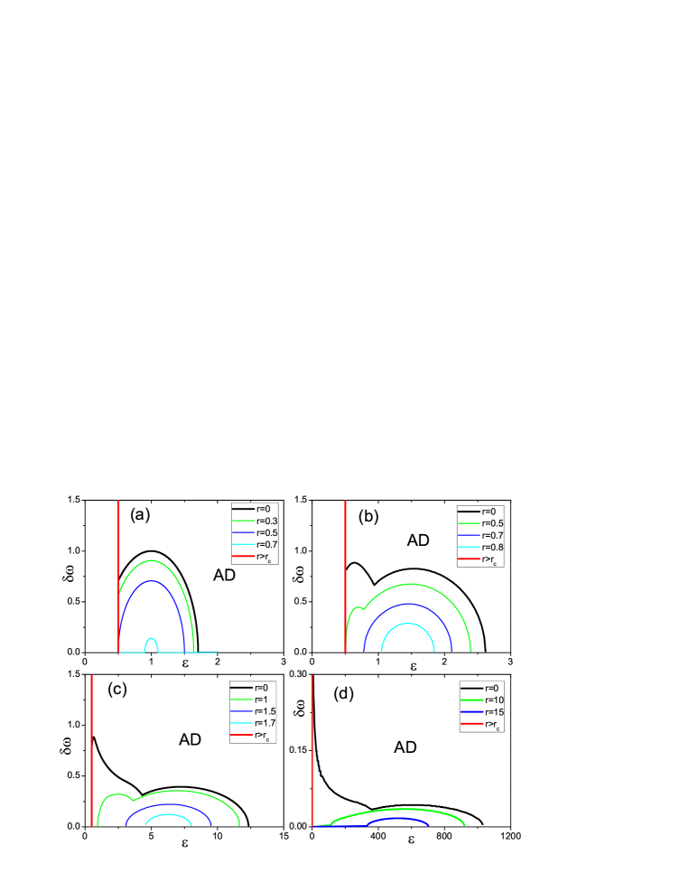
Figure 1: (Color online) The critical line of the AD in coupled system with non-flux boundary condition. The AD domain is the right and up part of the area enclosed by the line $\epsilon>0.5,\delta\omega>0$ and the critical lines of corresponding $r$. (a) $N=3$,$r=0$(black line),r=0.3 (green line),r=0.5 (blue line),r=0.7 (cyan line); (b) $N=4$,$r=0$ (black line),r=0.5 (green line),r=0.7(blue line),r=0.8 (cyan line); (c)$N=10$, $r=0$ (black line),r=1 (green line),r=1.5 (blue line),r=1.7 (cyan line); (d)$N=100$,$r=0$ (black line),r=1 (green line),r=2 (blue line),r=3 (cyan line),r=5 (magenta line).

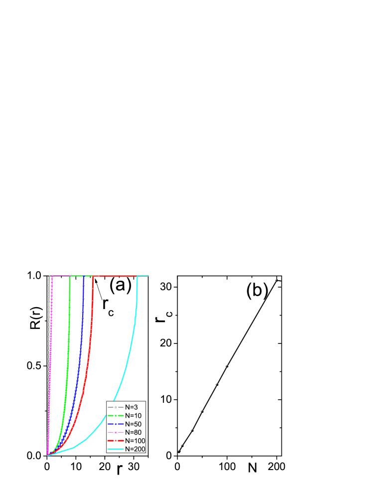
Figure 2: (Color online) (a) The normalized scaling factor $R(r)$ vs r for $N=3,10,50,80,100,200$, respectively. $R(r)=1-S(r)/S(0)$ with $S(r)$ standing for the area of non-AD island in parameter space $\epsilon\sim\delta\omega$ for $\epsilon>0.5$. For each given system size N, a monotonic increasing of R(r) vs r and a critical value $r_{c}$ are clear. All the data are numerically obtained by directly integrating the coupled system Eq.2. (b) The critical gradient coupling constant $r_{c}$ vs system size N. $r_{c}$ is linearly increasing with N.

Let’s firstly consider the gradient coupling effects on AD in the coupled system with non-flux boundary condition. The AD domain of parameter space $\epsilon\sim\delta\omega$ are calculated for different $N$ , $r$ in Eq.2 as shown in Fig.1(a)$\sim$(d) for $(N=3,4,10,100)$ respectively. The AD domain is the right and above part of area enclosed by $\epsilon\geq 0.5$(red solid line) and the curve line of corresponding $r$. The area enclosed by $\epsilon>0.5$ and the black solid curve for $r=0$ (marked with AD) in Fig.1 are the AD domain for $r=0$ which is right the AD domain of diffusive coupled system. Interestingly, we find that the AD region is monotonically expanding as the gradient coupling $r$ is gradually increasing until $r=r_{c}$, where $r_{c}$ is related to the systems size $N$. Thus, for an arbitrary given system size $N$, the gradient coupling may monotonically increase the AD domain for $r<r_{c}$. However, when $r\geq r_{c}$, the AD domain becomes the area enclosed by all $\epsilon>0.5$ and $\delta\omega>0$ and keeps constant for increasing gradient coupling strength $r$. Therefore, the gradient coupling tends to minimize the frequency mismatch needed for AD in diffusively coupled oscillators. According to Fig.1, there is another remarkable thing that smaller frequency mismatches $\delta\omega$ and larger diffusive coupling strength is needed for AD in the gradient coupled system with larger system size $N$ for arbitrary given constant $r$. However, based on these observations, we may predict the critical gradient coupling $r_{c}$ for each $N$. A normalized scaling factor is defined as $R(r)=1-S(r)/S(0)$, where $S(r)$ denotes the area of non-amplitude death island in the parameter space $\epsilon\sim\delta\omega$ for $\epsilon>0.5$. Obviously, $R(0)=0$. The relationship between $R(r)$ and r are presented in Fig.2(a) for different system size $N$. $R(r)$ monotonically increases with increasing $r$ until $r=r_{c}$, $R(r_{c})=1$. The critical gradient coupling $r_{c}$ has positive linear relationship with the system size $N$ as shown in Fig.2(b).

The AD domain of the gradient coupled system can be analytically presented according to $Re(\lambda_{i})<0$(the eigenvalues of matrix $B_{n}$) when the size $N$ is small, for example, $N=3,4$. When $N=3$, the eigenvalues of matrix $B_{n}$ are presented as follows,

$$\lambda_{1} = 1-2\epsilon+i(1+\delta\omega),$$

$$\lambda_{2,3} = 1-2\epsilon\pm\sqrt{2\epsilon^{2}-2r^{2}-\delta\omega^{2}}+i(1+\delta\omega)$$ (6)

Let $Re(\lambda_{i})<0$, the boundaries of the AD domain can be determined by following equations.
(1). Area I, if

$$\delta\omega^{2}\geq 2\epsilon^{2}-2r^{2}$$ (7)

then $\epsilon>0.5$
(2). Area II, if

$$\delta\omega^{2}<2\epsilon^{2}-2r^{2}$$ (8)

then

$$\epsilon > 0.5,$$

$$\delta\omega^{2} > 1-2(\epsilon-1)^{2}-2r^{2}$$ (9)

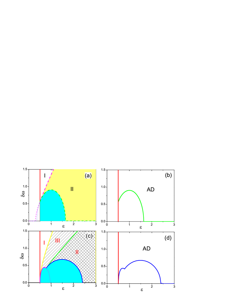
Figure 3: (Color online) The boundary line of the AD domain in coupled system with non-flux boundary condition. (a)Analytical results of the AD domain for $N=3r=0.3$(area I and II). magenta dashed line is Eq.7, green dashed line is Eq.Effects of gradient coupling on amplitude death in nonidentical oscillators. (b) Simulation results with parameters corresponding to (a). (c) Analytical results of the AD domain for $N=4,r=0.5$(area I,II and III). (d) Simulation results with parameters corresponding to (c)

Therefore, the AD domain for arbitrary given $r$ is composed of area I and II(AD domain for $r=0.3$ is presented in Fig.3(a), which is completely consistent with the numerical results as presented in Fig.3(b)). As $r$ increase from zero to $r_{c}$, the AD area II enclosed by Eq.Effects of gradient coupling on amplitude death in nonidentical oscillators enlarges monotonically. As $r>r_{c}$, AD is stable for all $\epsilon>0.5$ and $\delta\omega>0$ and keeps constant to increasing $r$. From Eq.Effects of gradient coupling on amplitude death in nonidentical oscillators, the critical gradient coupling $r_{c}$ of $N=3$ can be theoretically calculated as $\delta\omega^{2}\geq 0$ for all $\epsilon>0.5$, that is, $1-2r^{2}=0$,($r_{c}=\sqrt{1/2}=0.707$).

In the case of $N=4$, the eigenvalues of matrix $B_{n}$ can be given as

$$\lambda_{1,2,3,4} = 1-2\epsilon\pm 0.5\sqrt{Q_{1,2}}+i(1+3\delta\omega/2),$$

$$Q_{1,2} = 6\epsilon^{2}-6r^{2}-5\delta\omega^{2}\pm 2\sqrt{P},$$

$$P = (\epsilon^{2}-r^{2}-2\delta\omega^{2})(\epsilon^{2}-r^{2}-0.4\delta\omega^{2})$$ (10)

The boundaries of the AD domain can also be presented as areas I, II, and III according to $Re(\lambda_{1,2,3,4})\leq 0$.

(1) Area I, enclosed by Eq.Effects of gradient coupling on amplitude death in nonidentical oscillators;

$$\delta\omega^{2} \geq (\epsilon^{2}-r^{2})/0.4,$$

$$\epsilon > 0.5$$ (11)

(2) Area II, enclosed by Eq.Effects of gradient coupling on amplitude death in nonidentical oscillators.

$$\epsilon>0.5,$$

$$\delta\omega^{2}\leq(\epsilon^{2}-r^{2})/2,$$

$$\delta\omega^{2}>\frac{1}{9}(-20-6r^{2}+80\epsilon-74\epsilon^{2}$$

$$+2\sqrt{1584\epsilon^{2}-512\epsilon-2240\epsilon^{3}+192\epsilon r^{2}+64-48r^{2}+1189\epsilon^{4}-138\epsilon^{2}r^{2}-27r^{4}})$$ (12)

(3) Area III, enclosed by Eq.Effects of gradient coupling on amplitude death in nonidentical oscillators.

$$\epsilon > 0.5,$$

$$(\epsilon^{2}-r^{2})/2 < \delta\omega^{2}<(\epsilon^{2}-r^{2})/0.4,$$

$$\delta\omega^{2} > \frac{1}{4}(-10-6r^{2}-34\epsilon^{2}+40\epsilon$$

$$+2\sqrt{4r^{4}+16\epsilon^{2}r^{2}-24\epsilon r^{2}+6r^{2}+124\epsilon^{4}-264\epsilon^{3}+210\epsilon^{2}-72\epsilon+9}$$ (13)

The AD domain for $r=0.5$ is marked as area I, II and III in Fig.3(c) which is coincided with the numerical results in Fig.3(d) well. According to Eq.Effects of gradient coupling on amplitude death in nonidentical oscillators, the critical gradient coupling $r_{c}$ of $N=4$ can be determined by Eq.Effects of gradient coupling on amplitude death in nonidentical oscillators.

$$\frac{1}{9}(-20-6r^{2}+80\epsilon-74\epsilon^{2}$$

$$+2\sqrt{1584\epsilon^{2}-512\epsilon-2240\epsilon^{3}+192\epsilon r^{2}+64-48r^{2}+1189\epsilon^{4}-138\epsilon^{2}r^{2}-27r^{4}})=0$$ (14)

The solution of Eq.Effects of gradient coupling on amplitude death in nonidentical oscillators is Eq.15.

$$\epsilon=1\pm\frac{\sqrt{5}}{5}\pm\sqrt{0.7+0.3\sqrt{5}-(1+0.4\sqrt{5})r^{2}}$$ (15)

Since $\epsilon$ is real, then $0.7+0.3\sqrt{5}-(1+0.4\sqrt{5})r^{2}\geq 0$, that is $r_{c}=\sqrt{\frac{0.7+0.3\sqrt{5}}{(1+0.4\sqrt{5}}}=0.8507$.

IV. The periodical boundary condition

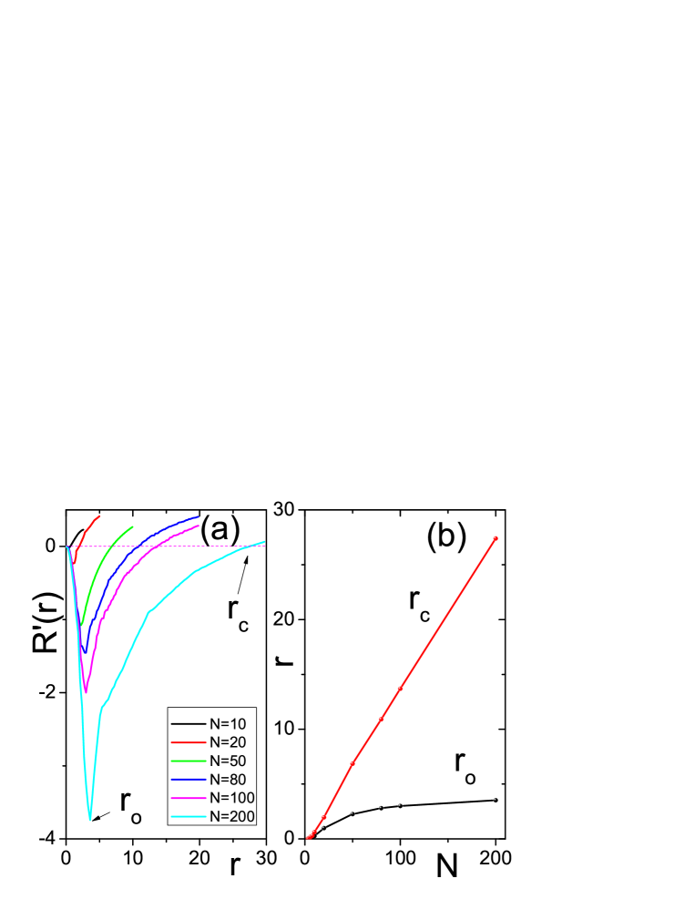
Figure 5: (Color online)(a) The factor $R^{\prime}(r)$ vs r for $N=10,20,50,80,100,200$ respectively. $R^{\prime}(r)=1-S(0)/S(r)$ with $S(r)$ standing for the area of non-AD island in parameter space $\epsilon\sim\delta\omega$ for $\epsilon\in(0.5,20),\delta\omega\in(0,20)$. For each given system size $N(N\geq 5)$, $R^{\prime}(r)$ firstly decrease to negative then increase to positive. There is a optimal gradient coupling constant $r_{o}$ which satisfy $R^{\prime}(r_{o})=R^{\prime}_{min}$ and a critical gradient coupling constant $r_{c}$ which satisfy $R^{\prime}(r_{c})=0$. (b) The optimal gradient coupling constant $r_{o}$ and the critical gradient coupling constant $r_{c}$ versus system size $N$($r_{o}=0$ when $N=3,4)$.

Now let’s explore the gradient coupled oscillators with periodical boundary condition. By checking the AD domain of parameter space $\epsilon\sim\delta\omega$ which is similar to that in Fig. 1 for $N=3,4,10,100$ as shown in Fig.4(a)$\sim$(d), where the AD region is the above part of area enclosed by line $\epsilon>0.5$ and the curve line of corresponding $r$. One may find that when $N=3,4$, the gradient coupling tends to decrease the AD domain monotonically as shown in Fig.4(a)(b), while for $N=10,100$, there is a critical gradient coupling constant $r_{c}$, within which the gradient coupling first increase then decrease the AD domain. That is to say, there is an optimal gradient coupling constant $r_{o}$ with which the coupled system has the largest AD domain in parameter space $\epsilon\sim\delta\omega$. However, when $r>r_{c}$, the gradient coupling begin to shrink the AD domain of formally diffusively coupled system. To quantified the critical gradient coupling constant $r_{c}$ and the optimal gradient coupling constant $r_{o}$ for different size $N$, a factor is defined as $R^{\prime}(r)=1-S(0)/S(r)$, where $S(r)$ is the area of the non-AD domain of corresponding $r$ for $\epsilon\in(0.5,20),\delta\omega\in(0,20)$. (Obviously, $R^{\prime}(0)=0$; $\frac{dR^{\prime}(r)}{dr}<0$ means the increasing $r$ enlarges AD domain; When $R^{\prime}(r)>R^{\prime}(0)$, the gradient coupling have smaller AD domain than the formally diffusively coupled system). Then $r_{c}$ is determined by $R^{\prime}(r_{c})=0$ and the optimal gradient coupling constant $r_{o}$ are determined by $\frac{dR^{\prime}(r)}{dr}|_{r=r_{o}}=0$. The relationship between $R^{\prime}(r)$ and $r$ for different system size $N$ are presented in Fig.5(a). Obviously, there is system size related $r_{o}$ and $r_{c}$. The detail relationship between $r_{o}$ and $r_{c}$ and system $N$ are presented in Fig.5(b). $r_{c}$ is linearly increase with $N$. $r_{o}=0$ for $N=3,4$ and increases nonlinearly with increasing $N$.

Accordingly, the AD domain can be predicted for small system size for example $N=4$. The eigenvalue of $B_{p}$ can be presented as follows,

$$\lambda_{1,2,3,4} = 1-2\epsilon\pm 0.5\sqrt{T_{1,2}}+i(1+1.5\delta\omega),$$

$$T_{1,2} = 8\epsilon^{2}-8r^{2}-5\delta\omega^{2}\pm 4\sqrt{S},$$

$$S = \delta\omega^{4}-4\delta\omega^{2}(\epsilon^{2}-r^{2})+4(\epsilon^{2}+r^{2})^{2}.$$ (16)

The boundaries of the AD domain are determined by $Re(\lambda_{1,2,3,4})<0$. The value of $Re(\lambda_{1,2,3,4})$ has various forms for corresponding parameters.
(1) if $T<0$, i.e.

$$\delta\omega^{2}>\frac{4}{9}(-2r^{2}+2\epsilon^{2}+2\sqrt{r^{4}+34e^{2}r^{2}+e^{4}})$$ (17)

then $Re(\lambda_{1,2,3,4})=1-2\epsilon$
(2) if $T\geq 0$, i.e.

$$\delta\omega^{2}\leq\frac{4}{9}(-2r^{2}+2\epsilon^{2}+2\sqrt{r^{4}+34e^{2}r^{2}+e^{4}})$$ (18)

then

$$Re(\lambda_{1,2,3,4}) = 1-2\epsilon\pm 0.5\sqrt{T_{1,2}},$$

$$T_{1,2} = 8\epsilon^{2}-8r^{2}-5\delta\omega^{2}\pm 4\sqrt{\delta\omega^{4}-4\delta\omega^{2}(\epsilon^{2}-r^{2})+4(\epsilon^{2}+r^{2})^{2}}$$ (19)

Thus, the critical line of AD domain can be found by solving the equations $Re(\lambda_{1,2,3,4})\leq 0$. The AD domain consist of two areas
(1) Area I enclosed by solution of $\epsilon>0.5$ and Eq.17;
(2) Area II enclosed by solution of Eq.18 and Eq.Effects of gradient coupling on amplitude death in nonidentical oscillators($Re(\lambda_{1,2,3,4})\leq 0$ in Eq.Effects of gradient coupling on amplitude death in nonidentical oscillators)

$$\delta\omega^{2} \geq g(\epsilon,r),$$

$$g(\epsilon,r) = \frac{2}{3}(-18\epsilon^{2}+20\epsilon-2r^{2}-5$$

$$+2\sqrt{81\epsilon^{4}-144\epsilon^{3}+18\epsilon^{2}r^{2}+100\epsilon^{2}+16r^{2}\epsilon-32\epsilon+r^{4}-4r^{2}+4})$$ (20)

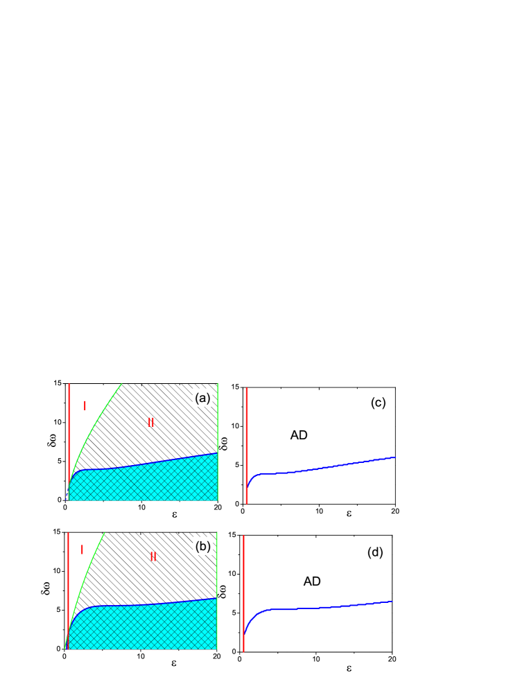
Figure 6: (Color online) (a)(b)Analytical result of the critical line of the AD domain in coupled system with periodical boundary condition and $N=4$. $r=5$,$r=10$ respectively. The AD domain is consisted of area I and area II. (c)(d) The simulation results of AD domain with parameter corresponding to (a) (b) respectively. The analytical results are consistent with the simulation results.

The AD domain of $r=5,10$ is presented as area I and II in Fig.6(a)(b), where area I is enclosed by $\epsilon>0.5$ and Eq.17, while area II is enclosed by Eq.18 and Eq.Effects of gradient coupling on amplitude death in nonidentical oscillators. It is also well consistent with the numerical results as shown in Fig.6(c)(d) respectively.

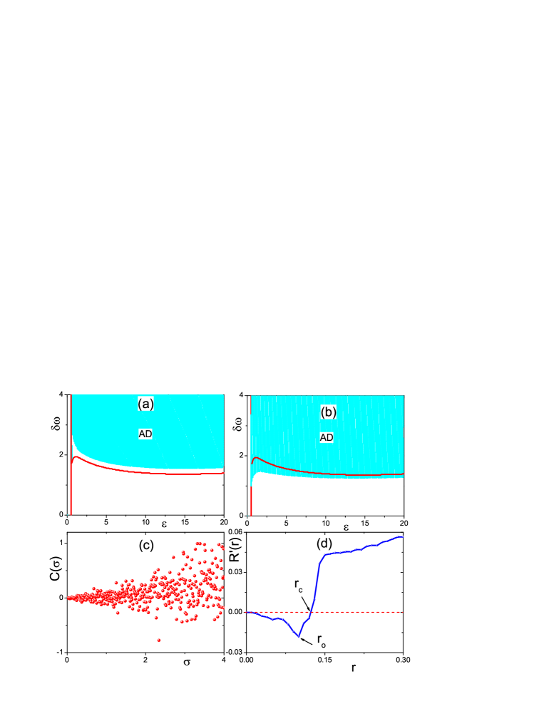
Figure 7: (Color online) (a)(b) The effects of noise intensity on AD domain for gradient coupled oscillators with periodical boundary conditions($N=10$,$r=5$), AD domain of two realizations of noise with intensity $\sigma=2$(cyan region). The red curve is the boundary of AD without noise. The noise can either enlarge or shrink AD domain. (c)Factors $C(\sigma)=1-S(\sigma)/S(0)$ versus noise intensity $\sigma$. $S(\sigma)$ is the area of non-AD domain with noise intensity $\sigma$. The deviation of $C(\sigma)$ is increasing with deviation of AD domain area. The stronger noise increase the deviation of AD domain. (d) $R^{\prime}(r)$ versus r of the gradient coupled Rossler oscillators with periodical boundary conditions and $N=10$, where $r_{c}=0.124,r_{o}=0.1$.

It is necessary to make some discussion. For convenience of analysis, the frequency distribution is set as regular monotonic trend as in Ref.rub . To explore the influence of frequency distribution on the AD domain, the noise is added to each frequency. Set $w_{j}=w_{1}+(\delta\omega(j-1)+\xi)$, where $\xi$ is the gauss noise with strength $\sigma$, namely, $\langle\xi_{i}\rangle=0$,$\langle\xi_{i}(t)\xi_{j}(t^{\prime})\rangle=\sigma\delta_{ij}\delta(t-t^{\prime})$. The AD domain of $N=10$,$\sigma=2$,$r=5$ is presented in Fig.7(a)(b) for different realization of noise. Where the noise may either enlarge or shrink the AD domain for different realization of noise. To see the effects of the noise strength $\sigma$ on AD domain area, the factor $C(\sigma)=1-S(\sigma)/S(0)$ versus $\sigma$ is presented in Fig.7(c), where $S(\sigma)$ is the non-AD domain area for noise constant $\sigma$ for $\epsilon\in(0.5,1.5),\delta\omega\in(0,2)$. Obviously, with increasing noise intensity, the noise tends to enlarge the deviation of the factor $C(\sigma)$, the effects of noise on the AD domain deviation is positively related to the noise intensity $\sigma$. Secondly, we may point out that the gradient coupling effects on AD domain is not exclusively existing in the coupled periodical oscillators but also existing in gradient coupled chaotic oscillators such as Rossler system $dx/dt=wy-z,dy/dt=wx+0.165z,dz/dt=0.2+z(x-10)$ with the coupling scheme as described in Eq.1, where $w_{j}=1+(j-1)\delta\omega,j=1,2,...,N$. The factor $R^{\prime}(r)$ defined above ($S(r)$ is the non-AD domain area for corresponding $r$ for $\epsilon\in(0.5,1.5),\delta\omega\in(0,2)$) versus gradient coupling constant $r$ for $N=10$ coupled Rossler oscillators with periodical boundary condition is presented in Fig.7(d) where the increasing $r$ firstly decreases then increases $R^{\prime}(r)$, which indicate that the gradient coupling first enlarge then shrink the AD domain area of coupled Rossler system. Moreover, there is also an optimal gradient coupling constant $r_{o}=0.1$ and a critical gradient coupling constant $r_{c}=0.124$.

Conclusion

The effects of gradient coupling effect on AD domain in an array of coupled nonidentical is strongly related to the boundary conditions. With no-flux boundary conditions, the gradient coupling tends to monotonically enlarge the AD domain in the parameter space $\epsilon\sim\delta\omega$ within the critical gradient coupling constant $r_{c}$. When $r>r_{c}$, the gradient coupling has no effects on AD domain any more. With the periodical boundary conditions, there is also a critical gradient coupling constant $r_{c}$. When $r>r_{c}$, the gradient coupling tends to shrink the AD domain. When $r\leq r_{c}$, it first enlarges then decreases the AD domain, that is, there is an optimal gradient coupling constant $r_{o}$ to realize largest AD domain for $N\geq 5$. The AD domain of those gradient coupled system are analytically predicted for small system size number. The remarkable thing is that the effects of gradient coupling on frequency mismatches caused AD is quite different with that on the time-delay induced ADzou where gradient coupling monotonically decreases the AD domain till completely eliminates AD. Ref.rub point out that the frequency mismatch $\delta\omega$ is beneficial to the AD, that is, larger $\delta\omega$ is easier to become AD in diffusively coupled array of oscillators. In this work, one may find that the gradient coupling is helpful to AD dynamics since smaller frequency mismatches $\delta\omega$ is needed for AD with proper gradient coupling constant. The gradient effects on the AD in coupled non-identical oscillators would be practically valuable to the dynamics control.

Acknowledgement

Weiqing Liu is supported by NSFC (Grant Nos 10947117,11062002) and Science and Technology Project of Educational Department Jiangxi Province(Grant No. GJJ10162); Lixiang Li is supported by the Foundation for the Author of National Excellent Doctoral Dissertation of PR China (FANEDD) (Grant No. 200951), and Specialized Research Fund for the Doctoral Program of Higher Education (No. 20100005110002).

Reference

Figure 4: (Color online) The critical line of the AD in coupled system with periodical boundary condition. The AD domain is the right and up part of the area enclosed by the line $\epsilon>0.5$ and the critical curve lines of corresponding $r$.(a) $r=0,5,10,15$ ,$N=3$. (b) $r=0,5,10,15$, N=4. (c) $r=0,0.4,1,5,10$, N=10; (d) $r=0,0.5,1,2,5,10,15$,N=100.

References

- (1) Winfree A T 1980 The Geometry of Biological Time Springer-Verlag, New York
- (2) Kuramoto Y 1984 Chemical Oscillations, Waves and Turbulence Springer, Berlin
- (3) Pikovsky A, Rosenblum M and Kurths J 2001 Synchronization: A Universal Concept in Nonlinear Dynamics Cambridge University Press, Cambridge, England
- (4) Bar-Eli K 1985 Physica D 14 242
- (5) Ullner E, Zaikin A, Volkov E I and Garc a-Ojalvo J 2007 Phys. Rev. Lett. 99 148103
- (6) Koseska A,Volkov E and Kurths J 2009 Europhys. Lett. 85 28002
- (7) Koseska A, Volkov E and Kurths J 2010 Chaos 20 023132
- (8) Ermentrout G B 1990 Physica D 41 219-231
- (9) Rubchinsky L and Sushchik M 2000 Phys. Rev. E 62 6440
- (10) Yang J Z, 2007 Phys. Rev. E 76 016204
- (11) Fatihcan M A, 2003 Physica D 183 1 C18
- (12) Hou Z and Xin H 2003 Phys. Rev. E 68 055103R
- (13) Liu W Q, Wang X G , Guan S and Lai C-H 2009 New J. Phys. 11 093016
- (14) Yang J Z, Hu G and Xiao J H 1998 Phys. Rev. Lett. 80 496
- (15) Xiao J H, Hu G, Yang J Z and Gao J H 1998 Phys. Rev. Lett. 81 5552
- (16) Zhan M, Hu G and Yang J Z 2000 Phys. Rev. E 62 2963
- (17) Zhan M, Gao J H, Wu Y and Xiao J H 2007 Phys. Rev. E 76 036203
- (18) Zou W and Zhan M 2008 Europhys. Lett. 81 10006
- (19) Motter A E, Zhou C S and Kurths J 2005 Europhys. Lett. 69 334; 2005 Phys. Rev. E 71 016116
- (20) Wang X G, Liang H, Lai Y C and Lai C H 2007 Phys. Rev. E 76 056113
- (21) Xingang Wang, Cangtao Zhou and Choy Heng Lai, 2008 Phys. Rev. E 77 056208
- (22) Zou W, Yao C G and Zhan M 2010 Phys. Rev. E 82 056203
- (23) Ramana Reddy D V, Sen A and Johnston G L 1998 Phys. Rev. Lett. 80 5109
- (24) Konishi K 2003 Phys. Rev. E 68 067202
- (25) Karnatak R, Ramaswamy R and Prasad A 2007 Phys. Rev. E 76 035201R
- (26) Zou W, Wang X G, Zhao Q and Zhan M 2009 Fron. Phys. China 4 97
- (27) Liu W Y, Xiao J H and Yang J Z 2004 Phys.Rev.E 7 0 066211