SNUTP10-008
Holography of mass-deformed M2-branes
Sangmo Cheon, Hee-Cheol Kim and Seok Kim
Department of Physics and Astronomy & Center for
Theoretical Physics,
Seoul National University, Seoul 151-747, Korea.
E-mails: sangmocheon@gmail.com, heecheol1@gmail.com, skim@phya.snu.ac.kr
We find and study the gravity duals of the supersymmetric vacua of mass-deformed Chern-Simons-matter theory for M2-branes. The classical solution extends that of Lin, Lunin and Maldacena by introducing a quotient and discrete torsions. The gravity vacua perfectly map to the recently identified supersymmetric field theory vacua. We calculate the masses of BPS charged particles in the weakly coupled field theory, which agree with the classical open membrane analysis when both calculations are reliable. We also comment on how non-relativistic conformal symmetry is realized in our gravity duals in a non-geometric way.
1 Introduction
With recent advance in M2-brane physics from Chern-Simons-matter theories [1, 2], it became clear that many essential aspects of M2-branes can be understood only when we have good controls over strongly coupled quantum field theories. The strong coupling physics is crucial in supersymmetry enhancement and appearance of M-theory states from monopole operators [2, 3, 4, 5, 6, 7], the partition function and Wilson loops on [8], determination of exact R-symmetry in theories [9], the degrees of freedom [10, 11, 12], to list a few examples. Analogous phenomena are either absent or turn out to be substantially simpler in 4 dimensional Yang-Mills theories for D3-branes. Also, the physics often depends on the Chern-Simons level in a more nontrivial way than the Yang-Mills coupling constant.
The roles of strong coupling dynamics turn out to be even more important for understanding M2-brane systems with mass gap. The simplest M2-brane theory with a mass gap is the mass-deformed Chern-Simons-matter theory [13]. This theory has many discrete supersymmetric vacua, whose classical solutions are first found in [14] and refined in [15]. When Chern-Simons level is , the gravity duals of the supersymmetric vacua are found by Lin, Lunin and Maldacena [16]. See also [17]. A puzzle was that the number of the gravity solutions is much smaller than that of the classical field theory vacua found in [14]. This puzzle was recently resolved in [15]. Many classically supersymmetric vacua of [14, 15] dynamically break supersymmetry, after which one obtains a perfect agreement between the supersymmetric vacua of gauge theory and gravity at .111It might sound surprising that the theory admits dynamical supersymmetry breaking. The analysis of [15] is from the ‘UV completion’ of this theory (Yang-Mills Chern-Simons-matter theory) which can have no more than supersymmetry. The result remains the same as one flows to IR, continuously taking the Yang-Mills mass scale back to infinity.
The analysis of [15] provides the partition function (or more precisely, the index) of supersymmetric vacua at arbitrary Chern-Simons level , whose gravity duals are not well understood. The goal of this paper is to identify and study the gravity duals of mass-deformed theory at general coupling .
Our results are very simple. The gravity duals for general can be obtained from those for [16] by introducing quotients, similar to the conformal Chern-Simons-matter theory [2]. This fact has been already noticed and partially studied in [18]. Another important aspect is that, contrary to the orbifold of , the orbifold of the mass-deformed geometry has fixed points of the local form . To correctly understand the gravity duals, one has to take into account the degrees of freedom localized on these fixed points. We find that fractional M2-branes [19] are stuck to some of these fixed points, which appear in the gravity solutions as discrete torsions. We find a set of gravity vacua which are in 1-to-1 map to the field theory vacua of [15], showing correct properties to be the gravity duals of the latter.
Having obtained the precise map between the gravity backgrounds and the field theory vacua, it could be possible to precisely address many questions on the gauge/gravity duality of this system. For instance, the vortex solitons [20, 18] in this theory have been studied from the gravity duals [18] using the probe D0-brane analysis at large . The results of this paper may help resolve some of the puzzles concerning these objects, raised in [18].
M2-brane systems with mass-gap could also have potential applications to low dimensional condensed matter systems. For instance, it is well known that quantum Hall systems admit a low energy description based on Chern-Simons theory. Addition of quasi-particles to this system would yield a Chern-Simons theory coupled to massive charged matters. There are some studies of (fractional) quantum Hall systems based on conformal Chern-Simons-matter theories [21]. As the quantum Hall systems are gapped in the bulk, it should be interesting to see if one can refine these studies with the mass-deformed M2-brane systems.
Having such future directions aside, we study some basic properties of various vacua, such as the spectrum of elementary excitations. After some part of the gauge symmetry is Higgsed in a vacuum, the unbroken part of the gauge group sometimes exhibits non-perturbative dynamics, similar to the confinement in Yang-Mills Chern-Simons theories studied in [22, 23]. This fact can be captured by recently studied Seiberg-like dualities in 3 dimensions [19], and also is correctly encoded in our gravity dual. We also study the gravity duals of massive charged particles, given by open membranes connecting various fractional M2-branes at the orbifold fixed points. The perturbative field theory analysis of BPS charged particles is reliable when the ’t Hooft couplings of unbroken gauge groups are small, while classical open M2-brane analysis is reliable when the membrane is macroscopic. We find a good agreement between the two spectra when both calculations are reliable. Although we only discuss BPS particles in this paper, similar comparison can be made with non-BPS particles.
The remaining part of this paper is organized as follows. In section 2, we first explain the results of [15] which identifies the supersymmetric vacua of the field theory. Then after explaining the gravity duals of the field theory vacua at , we introduce a orbifold and discrete torsions for general Chern-Simons level . Taking the fractional M2-branes into account, we show that the supersymmetric ground states of the gravity solutions perfectly map to the field theory vacua, with correct quantitative properties like symmetry or M2-brane charges. The general considerations are illustrated by some examples in section 3. In section 4, we study some elementary excitations in the context of gauge-gravity duality. A brief comment on non-relativistic conformal symmetry is also given. In section 5, we conclude with discussions on future directions. Appendix A summarizes the supersymmetry of gravity solutions and various probe branes. Appendix B explains the tensor description of the classical vacua. Appendix C presents the mass calculation of charged particles from the field theory.
2 The gravity soluions of mass-deformed M2-branes
Chern-Simons-matter theory with mass deformation preserving Poincare supersymmetry was constructed and discussed in [13, 14]. The theory has four complex scalars in bi-fundamental representations of the gauge group, where the subscripts and denote the Chern-Simons levels. The classical and quantum supersymmetric vacua of this theory have been studied in [14] and [15], respectively. At , the gravity duals of the quantum supersymmetric vacua are constructed in [16], which are asymptotic to in UV and exhibit complicated ‘bubbles’ of M2-branes polarized into M5-branes [24]. After semi-classical quantization of the 4-form fluxes, the discretized gravity solutions are in 1-to-1 correspondence to the supersymmetric vacua [15].
In this section, we review the supersymmetric vacua of the field theory identified in [15] for general , explain the gravity duals for obtained in [16], and present the generalization for arbitrary . Then we propose the map between the gravity solutions and the field theory vacua with various evidences.
2.1 Supersymmetric vacua of the field theory
Before mass deformation, there is an R-symmetry which rotates the four complex scalars (for ) in the fundamental representation. The mass deformation breaks this R-symmetry to , where and rotate and as doublets, respectively. See [13, 14, 15] for the details.
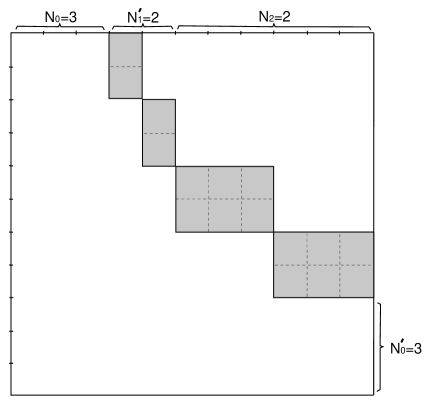
The classical supersymmetric vacua are given by scalar configurations with vanishing bosonic potential. The general solution is given by a direct sum of the following blocks. The blocks of first type are rectangular matrices with one more column, with . The blocks with denote empty columns. In this block, two scalars are taken to be zero, while the other two scalars are ( is the mass parameter [15])
| (2.1) |
Below, we shall call this the ’th block of first type. The blocks of second type are rectangular matrices with one more row, again with . Blocks with denote empty rows. Here the two scalars are zero, while
| (2.2) |
We shall call this the ’th block of second type. The classical supersymmetric vacua are parametrized by specifying how many blocks of different types and sizes are included in the direct sum. We denote by the number of the ’th block of first type, and by that of the ’th block of second type. An example of our parametrization is shown in Fig 1. As the direct sum (including empty rows and empty columns) should form an matrix, we obtain the following constraints on these ‘occupation numbers’ :
| (2.3) |
The first and second conditions are restrictions on the numbers of rows and columns. Equivalently, we obtain the following two constraints
| (2.4) |
which will be a more suggestive form for later interpretation.
Among these classical zero energy solutions, only some of them remain to be exactly supersymmetric at the quantum level. We take the Chern-Simons level to be positive without losing generality. The vacua which survive to be supersymmetric quantum mechanically should satisfy [15]
| (2.5) |
for all occupation numbers. Furthermore, when these restrictions are satisfied, the degeneracy (or more precisely the Witten index) of the supersymmetric vacua is
| (2.6) |
for given [15]. The total number of supersymmetric vacua with given rank (i.e. for a given theory) is the summation of the degeneracy of the form (2.6), taken for all occupation numbers satisfying (2.4) and (2.5).
One can also generalize the identification of supersymmetric vacua in [15] to the mass-deformed theory with gauge group, where [19]. The only change for the classical supersymmetric vacua is to replace (2.4) by
| (2.7) |
while the conditions (2.5) and the degeneracy (2.6) remain the same.
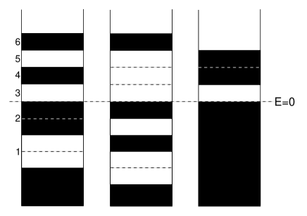

Another way of viewing these supersymmetric vacua is to use species of fermions, or ‘colored’ fermions, with occupation numbers , (for ) being either or . Being blind to the ‘color’ quantum numbers, one obtains the combinatoric factor (2.6) in the degeneracy by taking , . The first condition of (2.4) about the rank is simply the overall energy condition for pairs of chiral fermions in dimensions. As the energy level is half-integral, the fermions are in the Neveu-Schwarz sector. The second condition of (2.4) becomes the overall singlet condition for the sum over the color charges, where the particles with the occupation numbers carry charge and anti-particles with occupation numbers carry charge . In other words, this condition sets the sum of Fermi energy levels to be . For the theory with nonzero , the last condition modifies to setting the sum of Fermi levels to be . Such fermion viewpoint of the occupations can be illustrated as ‘droplets’ like Fig.2. In each droplet, an occupied sector with or is represented by filling the ’th level above/beneath the Fermi level (denoted by ) with a black/white stripe, respectively. In this example, the field theory occupation numbers are , , , , , , , and others zero.
One can also bosonize the colored fermions to chiral bosons on a circle, namely to compact bosons. The charges become the quantized momenta (for ) of bosons on the circle. The neutrality of overall (or sum of Fermi levels being ) corresponds to the restriction
| (2.8) |
The possible excitations of the bosons map to the so-called colored partitions of , which consists of Young diagrams with charges . The first condition of (2.4) on the energy of fermions can be rewritten in the bosonized picture as
| (2.9) |
where are excitations of the bosonic oscillators (not to be confused with fermionic occupations with same notation above), and are subject to the constraint (2.8). Note that the first term on the right hand side of (2.9) is the kinetic energy of zero modes.
In the bosonized picture, it is easy to calculate the partition function for the supersymmetric vacua, which trades the energy with the chemical potential as . The partition function for the compact bosons with net momentum is
| (2.10) |
The first factor comes from the Young diagrams, while the second factor is from the kinetic energy of zero modes. This is a generalization of the result of [15] for . For , agrees with the degeneracy of the gravity solutions of [16], as shown in [15]. Strictly speaking, the above vacua are obtained by deforming the theory appropriately, under which only the Witten index is invariant. So this partition function is the Witten index of the field theory.
2.2 Gravity solutions
The gravity solutions for the supersymmetric mass-deformed M2-branes at Chern-Simons level , all asymptotic to , are obtained in [16]. The metric and the 4-form field are given by 222The 4-form flux corrects the expression in [16], which we think should contain typos. In particular, we explicitly checked that the latter 4-form is not closed.
| (2.11) | |||||
where , denote length elements or volume 3-forms of unit round 3-spheres, which we call , . Various functions in the solution are determined by two functions , ,
| (2.12) |
The functions and are given by , . Note that, compared to the solutions presented in [16], a parameter with dimension of mass is restored. This could be eliminated to, say , by using the asymptotic conformal symmetry. will be identified with the mass paremeter appearing in the field theory [15] as .

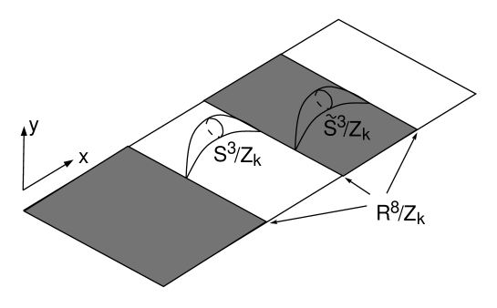
From the metric in (2.2), is proportional to the product of the square-radii of and . Therefore, at least one of the two 3-spheres shrink at . For the geometry to be smooth with a shrinking 3-sphere, the 3-sphere should combine with the radial direction () to form . This requires the function in (2.12) to have the boundary condition , where or shrinks for sign, respectively [16]. At the line parametrized by at , we therefore denote the parts with boundary behaviors by black/white regions, as shown in Fig 3. To visualize the regions better, we add a fictitious line segment to make the line look like an infinite strip of ‘droplet.’ In type IIB dual, this extra segment has the meaning of a spatial direction called in [16], which is T-dualized to one of the spatial coordinates of in (2.2). To have asymptotic , one should have a semi-infinite black region at one end and a white region at the other end. At the boundary of the adjacent black and white regions (call it for ), both 3-spheres shrink and appears near , by combining the two 3-spheres with .
There are various topological 4-cycles in this solution. Consider first a segment in the plane ending on different black regions at , and attach the 3-sphere to it, like the cycle on the left side of Fig 3. As shrinks at the ends of the segment, the 4-cycle smoothly wraps up, forming a 4-sphere. Similarly, one can consider a segment ending on different white regions at and attach to it, which also becomes a 4-sphere as shown by the cycle on the right side of Fig 3. Nonzero 4-form fluxes are applied through these 4-spheres, which have to be quantized. Below, we explain this quantization directly in M-theory. Similar discussion was provided in [16] from the type IIB duals.
Consider a 4-sphere containing which surrounds a black region () between and , where : see the cycle on the right side of Fig 3. As the 4-form field is closed, we can deform the 4-sphere without changing the 4-form flux over the cycle. We take the two points of the 4-sphere at to end exactly at the boundaries of the black region. We also deform the whole 4-sphere to . Near this black region, with small , one obtains
| (2.13) |
Other functions are given by
| (2.14) |
Here, from
| (2.15) |
one finds that
| (2.16) |
One can easily check that for , implying that is an increasing function there. The case with (with ) can be regarded as the semi-infinite black region, in which only the upper boundary exists at . The 4-form flux through the 4-sphere surrounding ’th black region is given by
| (2.17) | |||||
where we integrated by parts at the last step, using . For , one finds that the boundary contribution from the first term is zero, and the flux is proportional to the ‘length’ of the black strip. This is basically the result of [16] from the type IIB dual. For , the boundary term from is nontrivial. We temporarily set large but finite as a regulator. contribution there is expanded as
| (2.18) |
Thus, the flux through this non-compact 4-cycle is given by
| (2.19) |
times the total lengths of all finite black regions. The type IIB picture [16] that the flux is proportional to the area (or length in our case) of the black region is true only for finite 4-cycles.
Similarly, one can calculate the flux through 4-spheres containing which surround white regions. On the white region between and (, where the last entry is the semi-infinite white region), the functions are expanded near as
| (2.20) |
where the functions now satisfy . Other functions are given by , . The flux is given by
| (2.21) |
For with finite white regions, the boundary terms are zero so that minus of the length of the strip gives the flux. For the semi-infinite white region with , one obtains
| (2.22) |
which is the total length of the finite white strips.
The quantization condition of the 4-form fluxes on the 4-spheres is
| (2.23) |
where is the Planck length. The lengths of finite black/white regions are thus quantized as
| (2.24) |
In terms of the M2-brane tension , one obtains
| (2.25) |
We shall later use the rescaled coordinates of the boundaries
| (2.26) |
The distances between all boundaries are integers in the last coordinate.
2.3 Discrete torsions and fractional M2-branes
So far we have reviewed the solutions dual to vacua. For general , obvious solutions preserving the desired supersymmetry are the orbifolds of the above solutions. See appendix A for the reduction of supersymmetry. We are not aware of an argument that such orbifolds should give all geometries. Here we simply assume this fact and show in later sections that they are sufficient to understand aspects of dual field theory (e.g. vacua, symmetry, elementary excitations), which strongly implies that orbifolds of (2.2) are enough.
To take the orbifold, we consider the Hopf fibrations of , , and take the two angles of the fibers to be periodic , . The orbifold acts as
| (2.27) |
In the asymptotic region, in which and combine with one of the , coordinates to form a round 7-sphere, this orbifold acts freely on the Hopf fiber angle of , which is the known orbifold of [2]. However, the orbifold has fixed points in the full mass-deformed geometry (2.2). Namely, near and at the boundaries of black/white regions, and combine to form , where can shrink. The origin of is a fixed point of the orbifold.
With quotient, let us reconsider the 4-form fluxes through various 4-cycles. Considering the covering space of , the flux quantization over 4-cycles still requires (2.24) for the droplet. When the two ends of the segment for the 4-cycle are placed exactly at the boundaries of black/white regions as shown in Fig 4,
one can also consider the 4-cycle which wraps only. Such ‘4-cycles’ have two orbifold singularities of the form inherited from at the two ends, which we call north and south poles of . The 4-form flux through this is an integer divided by , which is fractional in general. This fractional flux through can be consistent with the flux quantization as one can turn on nonzero discrete torsions of the 3-form field at the two [19]. Discrete torsion on is given by the holonomy of on the torsion 3-cycle ,
| (2.28) |
where is an integer which can be put in, say, by a gauge transformation . The shift is recently claimed to be important [25] due to the so-called Freed-Witten anomaly, which is also consistent with the large gauge transformation of Page charges. times this expression, , is the ‘Page charge’ for the M5-branes wrapping a collapsing 3-cycle in [25]. One can turn on such a discrete torsion at each fixed point. Let us call the discrete torsion at the fixed point . The discrete torsions and on the adjacent fixed points in direction are related, due to the flux conditions on cycles just mentioned. The flux on the orbifolded 4-cycle stretched between and is
| (2.29) |
where the integrals on the right hand sides are taken with the outgoing orientations from the north/south poles. The left hand side is an integer divided by . As the two terms on the right hand sides are torsions at , up to integer shifts, we arrive at the recursion relation between adjacent discrete torsions
| (2.30) |
where the signs are for the black/white regions, respectively. From these relations, all torsions on the fixed points can be decided once we know the discrete torsion of the asymptotic , either at , .
The asymptotic discrete torsion at , which we call , is related to the rank of the gauge group in the dual field theory [19]. Namely, taking the torsion in with , the field theory comes with group.333We work with the convention of [25], which is different from [19], related to the sign choice in (2.28). Using (2.30), one can start from at and proceed by increasing , determining in turn. As the recursion formula (2.30) is given in the ‘outgoing’ convention from the edge, we should change before applying this formula. The torsion at is given by
| (2.31) |
Next, since the flux on the first white region is , one obtains
| (2.32) |
and so on. One can continue this analysis to obtain
modulo , where (black)i and (white)i denote the quantized lengths of the ’th black and white regions. In particular, the torsion at is given by
From , we find that the torsion at is in the outgoing orientation from infinity towards the droplet, agreeing with the torsion at .
In [19], it was argued that discrete torsions on can be interpreted as fractional M2-branes at the orbifold. In our case, we should be careful to identify whether discrete torsions are to be identified as fractional M2-branes or anti M2-branes. By anti M2-branes, we mean those which carry negative M2-brane charges in the convention that the total M2-charge of the gravity solution is positive. As the issue of orientation is same for both full and fractional M2-branes, we consider full M2-branes to understand the charge signs of fractional M2-branes.
Let us first consider the dynamics of probe M2-branes (full branes, not fractional) in the background (2.2). These M2-branes are extended in with two possible orientations, and are transverse in the 8 dimensional space spanned by and , . One obtains the following potential energy density from the Nambu-Goto action and the Wess-Zumino coupling,
| (2.33) |
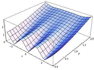
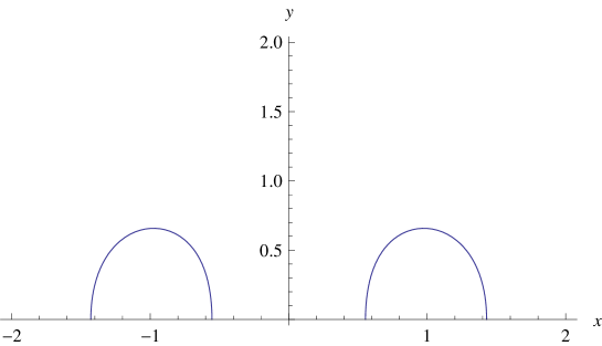
where the upper/lower signs are for the M2- and anti M2-branes, respectively. The signs for M2- and anti M2-branes can be easily determined by demanding the two contributions from and have more cancelation for M2’s than anti-M2’s in the UV region. This should be the case since the former has two contributions exactly canceling with each other in without mass deformation. From these potentials, one finds that M2-branes stabilize at and , while anti M2-branes stabilize at and . Fig 5 shows the potentials for M2- and anti M2-branes for the droplet with 5 edges.
The supersymmetry analysis of appendix A shows that both M2-branes (at odd edges ) and anti M2-branes (at even edges ) are supersymmetric. This is because the supersymmetry condition of the gravity solution reduces to with different signs at odd and even edges, making M2’s and anti-M2’s supersymmetric there. Therefore, we conclude that the fractional M2-branes at odd and even edges have same orientations as the full branes there. The BPS M2-branes with negative charge have a natural interpretation, on which we shall elaborate in section 3. As we shall illustrate in more detail there, we claim that gravity solutions containing negatively charged fractional M2-branes have to be excluded for comparing with the field theory vacua. A simple reasoning is that (either full or fractional) anti M2-branes with negative M2-charge in a background with positive charge can be geometrized to yield a solution which contains only positively charged fractional M2-branes. Therefore, solutions containing negatively charged M2-branes provide redundant descriptions of the field theory vacua.
Below in this subsection and also in section 2.4, we concentrate on the gravity solutions containing positively charged fractional M2’s only and show that they perfectly map to the supersymmetric field theory vacua with correct physical properties.
At a fixed point with torsion , the low energy effective description for these fractional M2-branes is pure Chern-Simons theory [19] with , in the convention of [25] that we are advocating. More precisely, this was derived with supersymmetric UV theory given by Yang-Mills Chern-Simons theory. In [19], this theory was argued to be Seiberg-dual to theory, by studying the D-brane realization of this system. In particular, this implies that the theory is dual to nothing. This could be closely related to the fact that Yang-Mills Chern-Simons theory with [22] and [23] gauge groups are confining. This aspect will be very important for us later when we try to map the gravity solutions to the field theory, as the low energy description of a field theory vacuum will also be given by Chern-Simons theories with products of like groups. We should have in mind that, the field theory factors of would be dual to nothing and thus absent in the gravity duals. Or oppositely, for the convenience of comparing our gravity solutions to the field theory vacua, we may work in the gravity dual side with some formally assigned ‘fictitious ’ Chern-Simons sectors as they are dual to nothing: the meaning of the last point will be clear below.
The droplets with nonzero torsions only at the ‘odd edges’ have a simple structure which will be useful later when comparing them to field theory. To simplify the story, we restrict our interest in the remaining part of this paper to the case in which the asymptotic torsion at is zero, with gauge group : the generalization to the case with is straightforward. We first note that, as even edges support zero torsions, the quantized distances between the even edges are all multiples of . This is easily seen from the recursion relation (2.30),
| (2.34) |
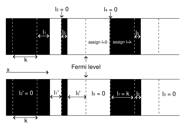
since all are . Therefore, we naturally divide the droplet into strips of length , as shown in the upper droplet of Fig 6 (where divisions are denoted by dashed lines). By construction, all even edges are boundaries of these strips. There could also be some boundaries of these strips which simply cut a long black or white regions into length strips. In each strip of length , there is a black strip of length on the left side and a white strip of length on the right side, for . The case with or happens when the whole strip of length is just white or black. When in a given length strip, is the torsion at or the number of fractional M2-branes, from (2.34). They are described by Chern-Simons theory. When or , we do not have to assign any such degree, as the fractional M2-branes are either absent or dual to nothing. Just for convenience, we also formally assign Chern-Simons theories even there: this will not affect the physics anywhere, as long as one remembers that theory is dual to nothing. In this way, we assign type Chern-Simons theories (or discrete torsion ) to all strips of length , not to the edges.
It is helpful to label the above strips of length by introducing the notion of Fermi level, which is obtained by taking all black strips down to fill the white regions below them, to get a droplet with one semi-infinite black and white regions only. The location of the boundary between the two semi-infinite regions is called the Fermi level. One can easily prove that the Fermi level is at one of the boundaries of the above strips of length , namely at a dashed line in Fig 6. To show this, recall that the torsion at is minus of the total quantized lengths of all black strips above (mod ), given by (2.31). The distance from to the other end of the neighboring white region is , so
| (2.35) |
from the relation between adjacent torsions. Since , one finds that
| (2.36) |
where the second equation is from (2.31). Now trying to pull down all black regions to fill in the whites below them, one first uses some of the black regions to fill the first white region of length . The remaining total lengths of finite black regions that can be pulled down is a multiple of , from the second equation in (2.36). Thus, after these remaining blacks are pulled down, the height of the Fermi level is a multiple of plus , which is at the boundary of the above strips of length , as claimed.
Now we parametrize the strips of length from the Fermi level. The strips above the Fermi level are labeled by non-negative integers , where increases as we get farther from the Fermi level. The strips below the Fermi level are labeled similarly, again by increasing non-negative integers as we move down away from the Fermi level. In each strip, the length of the black region contained in this strip is the discrete torsion assigned to this strip. Let us relabel the discrete torsions by denoting by the torsion in the ’th strip above the Fermi level, and by the torsion in the ’th strip below the Fermi level. When a strip consists of black or white regions only, we call the corresponding torsion to be or , respectively: remember that both are equivalent to no fractional M2’s.
At low energy, the fractional M2-branes in the bulk are described by pure Chern-Simons theory (having supersymmetric UV completion) with gauge group and level
| (2.37) |
One can also perform Seiberg duality transformations of [19] to obtain a different description, which will be more directly related to the field theory later. Performing this duality for all fractional branes below the Fermi level, and defining , one obtains a Chern-Simons theory with
| (2.38) |
gauge group and levels. An example of such a parametrization is given in the lower droplet of Fig 6. Below the Fermi level after Seiberg duality, the torsions assigned to a strip of length is given by the length of the white region in the strip. (2.38) takes the same form as the unbroken gauge symmetry of the field theory side [15], if one identifies , . More will be addressed about this map in the next subsection.
2.4 M2 charge, symmetry and map to the field theory vacua
Now we turn to the problem of mapping the gravity solutions to the field theory vacua explained in section 2.1. In this subsection, we provide three supporting evidences for our proposed map: symmetry, M2-brane charges, and the degeneracy of the vacua for given . In section 4, more evidence will be provided by comparing the spectra of elementary excitations of field theory and open membranes in the gravity duals.
We start by recalling that the low energy description in a field theory vacuum with first type blocks of size and second type blocks of size () is given by the Chern-Simons theory with gauge group and Chern-Simons levels [15]
| (2.39) |
Comparing this with the low energy Chern-Simons theory for fractional M2-branes in the gravity dual with gauge group (2.38), one is naturally led to consider the map
| (2.40) |
As both parameters and range between and , (2.40) provides a map between the classical gravity solution and a classical field theory vacuum solution which do not dynamically break supersymmetry. With this map, the gauge theory and gravity sides have same low energy descriptions with same symmetry groups and Chern-Simons levels.
Obviously, as the low energy descriptions are same on both sides, the vacuum degeneracy of the field theory and gravity precisely match with each other. For each factor of Chern-Simons theory, we consider it with a supersymmetric UV completion of an supersymmetric Yang-Mills Chern-Simons theory. The vacuum degeneracy of this Chern-Simons theory is given by [22, 26]
| (2.41) |
Therefore, both degeneracies from gauge theory and gravity are given by
| (2.42) |
agreeing with each other.
As the gauge group rank is given in terms of by (2.4), and as are identified with the torsions in the gravity solutions, one should also see if the M2-brane number calculated from gravity is consistent with (2.4). Discrete torsions (or fractional M2-branes) at various orbifold fixed points contribute to the M2-brane charge. This has been calculated rather recently in [27, 25]. We are interested in the Maxwell M2-brane charge,
| (2.43) |
where denotes the 7-sphere in the asymptotic region. If one computes this at asymptotic infinity, the calculation is the same as that obtained in without mass deformations. The result is [25] (see also [27])
| (2.44) |
where is the torsion. appearing in the first parenthesis is the M2-brane Page charge, with quantized [25]. In our case, with , one finds that
| (2.45) |
The number is the rank of the gauge group in the field theory.
On the other hand, in the full mass-deformed geometry, the M2-brane charge can also be computed with the IR data, from the droplets and torsions. To find this expression, we deform the integration 7-manifold in (2.43) to the IR region . As the Maxwell charge is not localized due to the equation of motion for ,
| (2.46) |
one obtains
| (2.47) |
is the shrinking region with , and is an 8 dimensional space spanned by and two 3-spheres, which has as its boundary. For , as the geometry is smooth, is void and the charge can be calculated solely from the last term of (2.47). For general , can be taken to be the union of small regions surrounding the singularities at the edges of black/white regions , .
The second contribution of (2.47) proportional to can be computed from the covering space of our quotient solution, which should be divided by . From the Young diagram picture of the droplet, this is simply given by the number of boxes in the Young diagram. See our section 2.1 as well as [16] for this conversion. From the ‘fermion droplet’ picture, the Young diagram size is the total ‘energy’ of all particles (black region above the Fermi level) and holes (white region below Fermi level) in the NS sector, as explained in section 2.1. For the droplet parametrized by , this quantity is given by
| (2.48) |
where shifts in all parentheses appear as fermions are in the NS sector.
With fixed points, there appear extra contributions from the singularities and discrete torsions contained in regions surrounded by . These have been computed in [27, 25] for each factor of , which also take the form of (2.44). Let us consider the contribution from a singularity at odd edges and even edges in turn. At an odd edge , there are no full M2-branes. Combining other contributions to , one obtains from (2.44)
| (2.49) |
where is the torsion ranged in . On the other hand, at even edges , the assigned torsion is zero from the requirement that no fractional anti M2-branes be there. So the only contribution is coming from the curvature at the singularity [27]. One can easily check that the curvature contribution comes with a relative minus sign compared to the odd edges,
| (2.50) |
One way to see this is continuously deforming the droplet to place an even edge on top of an adjacent odd edge. This can be done, ignoring the quantization of droplets, as the curvature contribution to can be obtained solely from classical considerations. As the two edges merge and annihilate, the curvature contributions from the two fixed points cancel, leading to the above sign flip. Summing over all contributions from the singularities, one obtains
| (2.51) |
In our new parametrization of the droplet/torsions with reference to the Fermi level, the torsions are to be identified with either or in our new parametrization introduced around (2.37). Although the latter set of torsions also include formally assigned extra torsions or , equivalent to nothing, they do not affect the expression in the summation as is zero for both . Also, this expression does not change by shifting to a Seiberg-dual description, changing to . One thus obtains
| (2.52) |
Adding this to (2.48), one obtains
| (2.53) |
Comparing this with the expression (2.45) obtained from UV, one obtains
| (2.54) |
This relation is exactly the same as the first equation in (2.4) for the field theory vacua, if we identify the torsions with the field theory occupation numbers . We find this is a very nontrivial consistency check of our proposal for the following reason. Our map was first based on the requirement that two low energy descriptions agree. However, the constraint from the same low energy descriptions is quite weak since one suffices to demand and with arbitrarily shuffled order. On the other hand, (2.54) demands that the subscripts of and be equal to have same .
The ‘level matching condition,’ the second equation in (2.4), can also be obtained from the gravity solution. Namely, is the length of the black region in ’th strip of length above the Fermi level, while is the length of the white region in ’th strip below Fermi level. By definition of the Fermi level, the total length of the black regions above the Fermi level equals that of the white regions below the Fermi level, leading to
| (2.55) |
This agrees with the second condition of (2.4).
We end this section with a comment on the unpolarized vacuum, where the classical expectation values of all scalars are zero. In this case, the only nonzero occupation numbers are and . This vacuum breaks supersymmetry if , namely when the gravity dual has a chance to be weakly curved. On the other hand, for , the unpolarized vacuum for M2-branes remains supersymmetric and is included in our gravity solutions. They necessarily have string scale curvature. Firstly in the UV region, this is true as the radius of curvature in the string unit is proportional to [2]. One can also check that the IR radii of curvatures in the region of various 2-spheres are small in the string scale. Extending one’s interest to vacua which spontaneously break supersymmetry, it should be interesting to find and study the gravity solution for the unpolarized vacuum with , trying to address the gravity duals of nonrelativistic conformal theories. See section 4.2 as well as the discussion section for more comments.
3 Examples
In this section, we provide concrete examples of the gravity solutions and their map to the field theory vacua, to supplement the formal considerations in the previous section. With various examples, we also argue why the gravity solutions containing negatively charged fractional M2-branes should be regarded as redundant solutions.
We start by noting that droplets can be equivalently described by Young diagrams, as explained in section 2.1 with Fig 2. The black/white regions map to the vertical/horizontal edges of the Young diagram. We use the compact Young diagram description for the illustration.

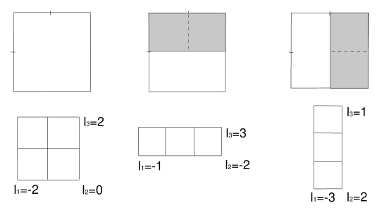
The examples for with various M2-brane charge are given as follows. Firstly, for , there is only one field theory vacuum . The corresponding Young diagram is made of one box, and its discrete torsion data is shown in Fig 8. After using to bring all torsions to be either or , the odd torsions carry M2-brane charge , while even torsions carry M2-brane charge . The numbers at the corners of the Young diagram are the discrete torsions , , at the singularities, which are defined mod 2. These can be obtained from the recursion relation (2.30).
For , there are three classical supersymmetric vacua which survive to be supersymmetric at the quantum level. The three vacua are given by , and . As scalar matrices, they look like the upper figures in Fig 8. The shaded boxes denote insertions of nonzero blocks. The Young diagrams have various numbers of boxes, which together with M2-charge from torsions should satisfy . Nonzero discrete torsions at convex corners of the Young diagram (i.e. even edges of the droplet) correspond to fractional anti M2-branes, carrying negative M2-brane charges. The gravity solutions which do not have fractional anti M2-branes are listed in the lower figures of Fig 8: each Young diagram map to the classical vacuum at the same column.

There are more gravity solutions with fractional anti M2-branes at the convex corners. These solutions at are shown in Fig 9. The torsion ranged in at a convex corner carries the M2-charge for anti M2-branes. For instance, the last Young diagram in Fig 9 has the M2-charge
| (3.1) |
Similar calculations yield for all other cases.
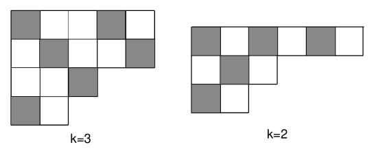
For all gravity solutions illustrated in Figs 8, 8, 9 by Young diagrams, and also for many other examples that we have checked with higher and , we empirically find that the M2-brane number is always given by the size of the so-called blended Young diagram with charge (the Chern-Simons level). The size of a -blended Young diagram is the number of boxes in a diagram forming diagonal lines with separation , as shown in Fig 10. For instance, for the left Young diagram at , we find and
| (3.2) |
which equals the size of the 3-blended partition (number of grey boxes). See, for instance, [28, 29] for more explanations on the blended Young diagrams.

Now let us consider the meaning of the gravity solutions which contain negatively charged fractional M2-branes. It is illustrative to start from a simpler case at , and put some full probe M2- and/or anti M2-branes in the background of [16]. An M2-brane in a background given by a droplet (Young diagram) is stabilized at one of the concave corners of the Young diagram, as the latter correspond to the odd edges of the droplet. As the full set of ground states is given by the solution of [16] parametrized by Young diagrams, adding an extra probe M2-brane at a concave corner provides a redundant description of the ground states. One can naturally identify the corresponding gravity solution which fully geometrizes the probe M2-brane. In the example shown on the left side of Fig 11, one geometrizes the probe by removing it and attaching an extra box at the same concave corner. Similarly, a BPS anti M2-brane with negative M2-brane charge at a convex corner can be geometrized by eliminating one box at that corner. Obviously, both configurations with probe M2- or anti M2-branes are redundant.
At general , fractional anti M2-branes cannot be fully geometrized, as we have been discussing in section 2. Positively charged fractional M2’s are indeed very essential for obtaining the gravity solutions dual to the field theory vacua. However, we find that all negatively charged fractional M2’s at convex corners can be eliminated to yield a geometry (Young diagram) with less boxes plus some extra fractional M2’s at concave corners. For instance, at , one can eliminate a box at each convex corner hosting nonzero torsion from the six Young diagrams in Fig 9, to obtain one of the Young diagrams in Fig 8. They reduce to
| (3.3) |
For , one sometimes has to eliminate more than one box at a convex corner. For instance, at , we find the reduction
| (3.4) |
The number of black dots in a diagram is the M2-brane number ( in this case) from the blended Young diagram for . On the left/right side, the discrete torsions are
| (3.5) |
where the bold-faced numbers are for anti M2-branes. The general rule that we find for eliminating the boxes from convex corners is to remove the maximal number of boxes without removing any box which contains a black dot.
4 Charged particles and their gravity duals
Having studied the vacua of this theory, it is then of interest to study the elementary excitations. In particular, we would first like to study the massive particles in various vacua, charged under the unbroken gauge group (2.39). When all ’t Hooft coupling constants , are small, one can simply diagonalize the mass matrix to understand their spectrum classically. This is subject to quantum correction when some couplings are large. For the BPS particles in the supersymmetric vacua with , one may expect to understand or test some aspects of the gauge/gravity duals that we proposed in the previous sections without much difficulty, hopefully relying on the weakly coupled field theory results.
However, even the BPS spectrum should also be studied with care. The first signal for the subtlety is that the Chern-Simons theory with gauge group and level (with supersymmetric UV completion given by Yang-Mills Chern-Simons theory) is dual to nothing [19] at low energy. This happens when the ’t Hooft coupling becomes . Therefore, naive classical spectrum for charged particles at small ’t Hooft coupling should break down even for BPS modes, whenever the relevant gauge group becomes . It is possible that the BPS spectrum could be nontrivial for particles charged under when . On the other hand, in some strongly coupled regime, the Seiberg like duality could allow one to study the spectra in dual descriptions with small coupling constants.
Turning to the charged particles from the gravity dual, it is natural to seek for such states from open M2-branes having two ends on fractional M2-branes in the background. In particular, we would like to have them wrap the ‘M-theory circle’ which is subject to the orbifold. By doing so, the open M2-branes reduce to fundamental strings heading towards two singularities at large . Near the tips of the orbifolds, the world-volumes of open M2’s ending on fractional M2-branes will be locally same as the open membranes dual to W-bosons in the Coulomb phase of conformal Chern-Simons-matter theories, studied in [30].
In section 4.1, we study classical configurations for the probe open membranes preserving half of the supersymmetry (6 real). Classically, their masses are given by the area of the membranes. There could in principle be subtle corrections from the two end points, over which we have little control. The classical analysis would be reliable when the membranes are macroscopic. In this case, one finds a good agreement with the results from weakly coupled field theory. See our section 4.1 for the subtle subleading terms and some comments on them.
In section 4.2, we briefly discuss possible non-relativistic conformal field theories in this gauge/gravity duality, as they have to do with taking the low energy limit keeping a subset of these massive particles. At each vacuum, one can take the non-relativistic limit keeping either ‘particle’ or ‘anti-particle’ modes with respect to a symmetry (to be identified with the particle number symmetry). The geometric realizations [31, 32] of holographic non-relativistic conformal symmetry do not appear to be relevant in our context, implying broader possibilities of holographic non-relativistic systems than those studied so far.
4.1 Spectrum of charged particles
Before presenting the analysis for the BPS spectrum of charged particles, we note that the vacua preserve global R-symmetry by mixing them with some global parts of the gauge symmetry. For the matrix block of first type, is realized on the and rows and columns of the gauge indices as totally symmetric representations. Similarly, for the matrix block of second type, is realized on the and rows and columns as totally symmetric representations. Detail on the tensor representations of the irreducible blocks is explained in appendix B.
We first study the massive vectors modes, which acquire nonzero masses through Higgs mechanism. We start by considering a classical vacuum containing an irreducible block of first type which is an matrix, and another block of first type which is an matrix. We find that the ‘off-diagonal’ matrix in and the matrix in mix with each other in the Gauss’ law, which becomes the classical equation of motion for massive vectors. The modes solving the Gauss’ law equation, after an appropriate gauge-fixing for scalars to be eaten up by vectors, have following masses and representations under :
| (4.1) |
where half-integral denotes the ‘total angular momentum’ quantum number for , and an integer runs over . Namely, there are two representations with given quantum number with different masses. Exceptionally, there is a representation with (i.e. ) with the mass . See appendix B for the derivation. One can do a similar analysis for the complex conjugate modes, after which we obtain the same representations and masses: this is obvious from the complex conjugation of the results above. After quantization, with the Chern-Simons term providing the symplectic 2-form, one of the conjugate pair would become the creation operator while the other becomes the annihilation operator.
The above result contains both BPS and non-BPS modes. The modes preserving some supersymmetry can be analyzed by studying the fermion supersymmetry variations. In the convention of appendix C, the supersymmetry is labeled by spinors with in the anti-symmetric representation of , broken to by the mass deformation. The spinor is subject to the reality condition . We investigate the -BPS modes preserving and its conjugate , where the subscript denotes the spatial spin part which diagonalizes . As analyzed in appendix A, these -BPS particles correspond to open M2-branes (or fundamental strings in the type IIA limit) which are smeared along base of . The open M2-branes localized on these 2-spheres are shown to be -BPS from the gravity dual, which is broken to after this smearing.444This is very similar to -BPS Wilson loops in smeared on . See appendix A. As we shall see in appendix C, our charged particles carry definite charges, inevitably delocalized on the 2-spheres. The modes preserving this supersymmetry exist only when , and among the above two representations, only one with
| (4.2) |
is BPS. This shall be reproduced from gravity when the classical membrane analysis is reliable.
The analysis of massive vector modes connecting two irreducible blocks of second type, with sizes and , is completely analogous to the above modes connecting two first type blocks of vacuum. The BPS mass is again given by for .
The massive vectors connecting an irreducible block of first type and an block of the second type come from the matrix part of , and also from matrix of . The numbers of rows and columns of the latter two matrices are the dimensions of irreducible representations of and , respectively. All masses are given by
| (4.3) |
Similar analysis can be done for the complex conjugate block of and block of , where we (obviously) obtain the same mass. Combining the conjugate modes and after quantization, one finds that only half of the two possible modes remain BPS. See again appendix C for the details.
Similar analysis for the BPS scalar modes can be done. The modes connecting two first type blocks, or two second type blocks, of sizes and have mass
| (4.4) |
while the modes connecting one first type and one second type blocks of sizes , have mass
| (4.5) |
The BPS masses are the same as the corresponding vector modes. See appendix C.
Now we study the same charged objects from the gravity dual. From the identification of the gauge symmetry, the natural candidates are the open M2-branes connecting fractional M2-branes at the orbifold fixed points. Such states exist only when . The open M2’s should be extended along a line in the plane and wrap the M-theory circle (i.e. diagonal direction of the two Hopf fibers of two 3-spheres). The resulting 2-dimensional spatial manifold is topologically . From the Nambu-Goto action, the energy of this open M2-brane is
| (4.6) |
The last line integral is the ‘length’ of the curve in the plane with the Euclidean measure. As the two ends of the curve are at where fractional M2-branes are located, the energy is minimized when the curve is a straight line . To compare this result with the field theory, let us Seiberg-dualize all the gauge groups below the Fermi level and label the fractional branes above/below the Fermi level by as explained in section 2.3, to go to the same duality frame as the field theory. For the open M2 connecting ’th and ’th fractional M2-branes above the Fermi level (with ), the mass is given by
| (4.7) |
Upon identifying , the first two terms in the parenthesis agrees with the weakly coupled field theory spectrum. The last two terms are 1-loop corrections. We are not completely sure which of the two calculations are valid between classical field theory and gravity at this subleading level. Strictly speaking, both calculations are valid when : otherwise, as there are sectors of strongly coupled Chern-Simons theory both from field theory and gravity sides, both calculations might be unreliable. Also, for classical M2-brane calculation to be reliable, we should have for the worldvolume of open M2’s to be macroscopic. When all the requirements for the validity of gauge/gravity calculations are satisfied, we find that the two results agree with each other.
At this point, we should mention that there are examples in which BPS masses receive quantum corrections at 1-loop level. In particular, in the context of Chern-Simons-matter theories, such a phenomenon is observed for BPS vortices when a symmetry is broken, together with the same correction to the central charge.555 We thank Choonkyu Lee for informing us of this result, which is in his unpublished work. It is not clear whether this implies that subleading terms in (4.7) should be seriously considered. More comments about the exact BPS spectrum is given at the end of this subsection, and also in the discussion section.
Similar analysis for the charged particles can be done for the open M2’s connecting fractional M2-branes below the Fermi level. The analysis is completely analogous to the above.
The last case to discuss is the modes connecting ’th fractional M2-brane above the Fermi level, and ’th fractional M2-brane below the Fermi level. Repeating the analysis above, one obtains the following mass from the classical M2-branes:
| (4.8) |
Comparing with the field theory spectrum , we first find a discrepancy proportional to the ’t Hooft couplings, which can be ignored in the weak coupling limit. Even after ignoring this part, another difference is that the field theory spectrum has compared to the classical gravity result. This is again subleading in the limit in which classical membrane analysis is reliable, again implying agreement between the two calculations.
Again it could be that the last subleading discrepancy between the field theory and gravity may have to be considered seriously, and one may want to clarify which of the two calculations has to be refined. As the field theory calculation is obviously reliable when ’t Hooft couplings are small, we suspect that classical gravity calculation has to be corrected, perhaps by taking into account some effects from the boundary of open M2-branes. A similar subleading discrepancy was observed in the conformal Chern-Simons-matter theory, in the study of the field theory dual of giant M2-brane torus. The last object can be regarded as open strings connecting spherical D2-brane dual giant gravitons [33], somewhat similar to our open M2’s as they are connecting spherically polarized M5-branes in the probe limit [24].
As shown in appendix A, the open M2-branes localized on base of are -BPS. On the other hand, as we smear the open M2-branes along the transverse 2-sphere, one only obtains -BPS solutions. The supersymmetry of the gravity and field theory sides thus agree with each other.
We remark that we have not clarified the degeneracies of various BPS particles from the gravity dual. One point which could be important is that open membranes are transverse to one of the two 2-spheres spanned by either or R-symmetries. By examining the 4-form flux of (2.2), we find that open M2’s effectively behave as charged particles moving on in nonzero magnetic fields. There are nontrivial degeneracies from the lowest magnetic monopole spherical harmonics. It could be possible to understand the degeneracies from the gravity dual in this way, which we leave as a future work.
Another point worth a consideration is that the gravity solution does not see the ‘Fermi level’ at all. Before performing Seiberg-like dualities for some fractional M2-branes in section 2.3, all fractional M2-branes are described by type Chern-Simons theories, where is the torsion at each orbifold fixed point. We have performed Seiberg-like dualities for the Chern-Simons theories living below the Fermi level of the droplet, to compare the gravity result with the field theory. The field theory in the last Seiberg-duality frame is weakly coupled when all , are much smaller than . In the gravity viewpoint, this means that the quantized lengths of all black regions above the Fermi level are much smaller than , while the lengths of all white regions below the Fermi level are smaller than .666Of course, such gravity solutions have Planck scale curvatures. So the notion of Fermi level emerges just by demanding the field theory be weakly coupled in a particular duality frame. At the full non-perturbative level, we think the field theory should also be ignorant about the Fermi level. To test this, one could rely on localization methods to calculate the partition function (or index) of all BPS particles. Similar to the instanton partition functions [28] in 5 dimensional Yang-Mills theories compactified on a circle, we may introduce an Omega deformation with the rotation on spatial part of to lift the translational zero modes of these particles. This partition function would include contributions from various vortices [20, 18] as well as elementary particles. Such a calculation could also resolve the puzzle raised in [18] about the zero modes (or more precisely ground state degeneracies) of vortices.
4.2 Remarks on non-relativistic conformal symmetry
The massive charged particles studied in the previous section are subject to various conservations of charges. In particular, the overall factors in the or type gauge groups turn out to be important when . As various massive particles are bi-fundamental in two factors of such unitary groups, the charge of a particle under a given is either , or .
In the symmetric vacuum, with in our notation, a non-relativistic limit was considered in [34, 35] which discards ‘anti-particle modes’ which are negatively charged under the baryon-like . See also [36] for further discussions on this theory. As is the global part of the difference between two overall ’s in [2], is a special combination of many ’s in the general Higgs vacua mentioned in the previous paragraph. Similar non-relativistic limits can be taken in the Higgs vacua that we have been discussing, in which scalar expectation values are nonzero. With various overall factors, one can keep the modes with definite signs of charges under various ’s and take a non-relativistic limit similar to [34, 35]. In the bosonic sector, one would obtain non-relativistic kinetic terms and quartic interaction terms of various modes. This system would have a scale symmetry with dynamical exponent . It should also have Galilean boost symmetry as well as the symmetries analogous to particle number mentioned above. In [34, 35], the non-relativistic system also has time special conformal symmetry. This appears when the relative coefficients of the Chern-Simons term, kinetic term and the quartic interactions are fine tuned. The general non-relativistic system from the Higgs vacua could also have this symmetry, although we have not performed this analysis.
The particle number-like symmetries are realized in the bulk as part of the gauge symmetry localized on fractional M2-branes. Note that this is in contrast to [31], in which an isometry of a spacetime direction is used to realize the particle number symmetry. This is because our gravity solutions for mass-deformed M2-branes do not fully geometrize the M2-brane charges into flux, but leave some of them as fractional M2-branes. We expect that other part of non-relativistic symmetries will not be geometrically realized, either. For instance, in [31], other symmetries also have nontrivial actions along the direction which realizes particle number isometry. Our system is also different from another recently studied non-geometric realization of the particle number [32], as our particle symmetry lives in dimensions.
After the suggestion of [31] on the gravity duals of non-relativistic conformal systems, there have been some attempts to obtain such solutions arising from mass-deformed M2-branes [37], having the symmetric vacuum theory of [34, 35] in mind. These works sought for solutions with some supersymmetry, and also with the isometry as a gravity dual of the R-symmetry of the system. Firstly, if one is studying the symmetric vacuum, one would have to study solutions with broken supersymmetry, as the field theory vacuum breaks supersymmetry for . Also, the reason why symmetry is imposed in [37] is because R-symmetry of the field theory at is reduced to for general . If this reduction of symmetry happens by a orbifold from the gravity dual like the solutions in this paper, then the ansatz one should consider is much more restrictive than those considered in [37]. It would be interesting to see if such a strong restriction would help us find non-supersymmetric gravity solutions.
5 Discussions
In this paper, we have shown that quotients of the polarized M2-brane solutions of [16] are dual to the supersymmetric vacua of the mass-deformed Chern-Simons-matter theories, after taking fractional M2-branes and strong coupling Chern-Simons dynamics into account.
As the gravity duals that we found in this paper have rich structures, we think this model can be studied for various purposes. In particular, it would be very interesting to see if we can extend or refine the studies on quantum Hall systems based on conformal Chern-Simons-matter theories [21], to the theories with mass gap. The latter should be desirable as the quantum Hall systems are gapped in the bulk. Also, it would be interesting to study various interface or defect configurations which support stable massless charged states at edges. and branes are used in CFT-based models [21]. As the mass-deformed geometry also has topological 4-cycles, M5-branes wrapping them would naturally provide dimensional defects in . Due to the presence of nonzero magnetic flux on such cycles, one has to attach M2-branes to the defect for tadpole cancelation of the 3-form world-volume field. These tadpole M2-branes are extended along half of , having the defect as their boundaries.
As explained in this paper with elementary excitations, studies of BPS particles in this theory expose rich structures and various subtleties. Although the leading energies for macroscopic open membranes agree with elementary excitation masses, we think it could be important to understand the exact spectrum from both sides. Another type of subtlety in the BPS spectrum was found in [18] in the studies of vortex solitons and D0-branes in the gravity dual. Namely, it has been shown that the dimensions of moduli spaces of the dual objects apparently seem to disagree, where the field theory and gravity show complex and dimensional moduli, respectively. This difference would yield different ground state degeneracies after quantization. To get an exact result for the spectrum of BPS particles in the field theory side, one can try a localization calculation for the index for these BPS states, similar to the instanton partition function counting BPS bound states of 5 dimensional supersymmetric Yang-Mills theories [28].
As discussed in section 3.2, it may not be too difficult to seek for the gravity solutions with non-relativistic conformal symmetry dual to the symmetric vacuum, breaking supersymmetry.
For supersymmetric mass-deformed Chern-Simons-matter theories, the S-matrices for the scattering of 2 to 2 particles in the ’t Hooft limit have been studied in [38] for the symmetric vacuum. In the Higgs phase vacua, various macroscopic open membranes could be used to carry out some semi-classical calculations. It would be interesting to study them, firstly in the theories discussed in this paper. Also, as mentioned in [38], S-matrix of the mass-deformed theory is well defined, in contrast to the conformal theories.
It is also possible to replace the orbifold by other orbifolds to yield the gravity duals of mass-deformed Chern-Simons-matter theories with reduced supersymmetry. The conformal or supersymmetric theories have moduli spaces given by orbifolds of . The mass-deformed geometries could simply be obtained by acting the same orbifold quotients on the solution of [16]. For instance, the theory replaces by a dihedral group [13, 19]. To classify and study these vacua from the gravity duals like our vacua, one should know the contributions of orbifold curvature singularities and the fractional M2-branes to the M2-brane charge. This would be a generalization of [27, 25] to other orbifolds, which is not done yet. The classical vacua of the mass-deformed field theories are not fully classified either, as far as we are aware of.
Acknowledgements
We would like to thank Dongmin Gang, O-Kab Kwon, Choonkyu Lee, Sangmin Lee, Sungjay Lee, Eoin O Colgain, Soo-Jong Rey, Tadashi Takayanagi and especially Ki-Myeong Lee for helpful discussions. We also thank Sungjay Lee for comments on the preliminary version of this manuscript. This work is supported in part by the Research Settlement Fund for the new faculty of Seoul National University (SK), the BK21 program of the Ministry of Education, Science and Technology (HK, SK), the National Research Foundation of Korea (NRF) Grants No. 2010-0007512 (SC, HK, SK), 2007-331-C00073, 2009-0072755 and 2009-0084601 (HK).
Appendix A Supersymmetry of gravity solutions and M2-branes
In this appendix, we explain the Killing spinor of (2.2), the projection after , the supersymmetry of probe M2- and anti M2-branes wrapping , and finally the supersymmetry of open M2-branes dual to the charged particles.
We take the 11 dimensional vielbein to be
| (A.1) |
where and . The right 1-forms on are
| (A.2) |
which satisfy and
| (A.3) |
on are similarly defined. 11 dimensional gamma matrices are taken to be
| (A.4) |
where and are and gamma matrices, respectively.
The supersymmetry of the gravity solutions discussed in this paper is studied in [17]. We independently checked all equations we use below. The algebraic half-BPS condition is given by
| (A.5) |
The coefficients satisfy
| (A.6) |
The sign of changes as one crosses a curve on the plane.
The Killing spinor can be written as , following the gamma matrix decomposition. It turns out [16, 17] that the Killing spinors can be decomposed into , depending on the sign of the conditions satisfied by the two dimensional spinors , on , :
| (A.7) |
The projection conditions to these components are given by
| (A.8) |
In the right 1-form basis, the vielbein of a unit 3-sphere is given by . The solutions to (A.7) are given by
| (A.9) |
with constant spinors , and simiarly for .
The quotient shifts . For the Killing spinors with sign, the components , are constants. But the frame given by (A.2) changes under the shift of . This implies that the Killing spinors , are not invariant under shift, apart from the special cases with . On the other hand, the spinors , have both components and frame basis changing under the shift. This structure makes the spinors all invariant under . To see this clearly, we rewrite the spinors in the left 1-form basis, , where
| (A.10) |
These satisfy . In this basis, it is easy to show that
| (A.11) |
with constant . Similar expressions can be obtained for . As the basis (A.10) is invariant under the shift, the fact that have constant components imply that the spinors with sign are invariant under . In this basis, the action on is given by
| (A.12) |
For the spinor to be invariant under this shift, the eigenvalues of , should be either or , reducing the Killing spinors to . Thus, only out of spinors preserve in total. The supercharges with correspond to , in the field theory , while the remaining supercharges are with , in the notation of appendix C.
To understand the supersymmetry of full or fractional M2-branes extended along , one should know when satisfies , where sign has to do with whether M2- or anti M2-branes is BPS. From (A.6), one finds that when . This happens at on the boundaries of black and white regions: near , , one can easily check that , proving our assertion. These are the points where we argued in section 2.3 that probe M2-branes are located (M2’s at and anti M2’s at ). We still have to check the sign of at each edge. From the analysis of the potential energy for these branes, we expect that M2-branes are BPS at odd edges while anti M2-branes are BPS at even edges . This indeed turns out to be the case. To see the change of the sign, we study the curve on the plane, where . This curve consists of various pieces which circles around all even edges . See Fig 12 for an illustration. Firstly, the M2-brane is BPS at asymptotic infinity. As the edge at is connected to infinity without crossing this curve, does not change sign and M2-branes are BPS there. Then, moving along the line increasing , one finds that at odd and even edges have opposite signs. This proves our expectation that M2- and anti M2-branes are BPS at odd/even edges, respectively. We also note that the half-BPS condition (A.5) locally becomes that for an M5-brane at , as there. It was also shown in [18] that probe D0-branes are stabilized at these curves, which is natural as D0 is mutually supersymmetric with D4-branes (type IIA reduction of M5).
We finally study the fraction of supersymmetry preserved by the open membranes discussed in section 4.1. We study those stretched in the white region: those stretched in the black regions can be analyzed in a similar manner. The worldvolume supersymmetry demands
| (A.13) |
On the white region, the condition (A.8) for the sector is , respectively. We should thus consider the projection condition for . As the projection on spinor is trivial, we should study the projection of on . Let us first consider the case in which the M2-brane’s position on the base of is localized. Without losing generality, one can put the M2 at . The projection condition (A.13) requires to take an eigenvalue of . In the right 1-form basis, the constant spinors containing can be trivially taken to be such eigenstates, yielding the -BPS condition similar to the field theory charge particles. The spinors containing at is given by
| (A.14) |
As the dependent part only contains , one can take and to be eigenstates. Therefore, collecting all sectors with signs, one obtains a half-BPS condition for open M2-branes localized on .
On the other hand, the field theory charged particles discussed in section 4 are all delocalized on , as they are in definite angular momentum eigenstates. For an open M2-brane whose location on base of is smeared, the projection appearing in (A.13) cannot be imposed at every point on for , as the matrix does not commute with . So supersymmetry appears only in the sector, making this object -BPS (with 2 real supercharges from ).
The above reduction of -BPS to -BPS open M2-branes after smearing is very similar to reduction to the -BPS Wilson loops in smeared on [39].
Appendix B tensor representation of the vacua
In this appendix, we present the tensor representations of the irreducible vacuum blocks, which is convenient for the group theoretical analysis in appendix C.
Our basic goal is to explain that the irreducible block is a trivial representation of , if we regard the or indices for rows/columns as symmetric tensors or ranks and . To show this, we start by rewriting matrices as
| (B.1) |
where all and type indices are symmetrized and assume either or . To get back and forth between the dimensional vector and rank symmetric tensor basis with correct normalization, we introduce the normalized basis for symmetric tensors
| (B.4) | |||||
| (B.9) |
for , which satisfies . The symmetrization of a rank tensor is attained by the projection
| (B.10) |
which is
| (B.15) |
Here, and written above or denote the numbers of repeated indices. As the normalized basis for symmetric tensors corresponds to the normalized basis for the dimensional unit vectors, the dimensional vector component (for ) is given in terms of tensor components as
| (B.16) |
Therefore, the matrix elements are given in terms of symmetric tensors by
| (B.17) |
In this tensor form, we claim that the vacuum block is given by
| (B.18) |
To show this, we study the matrix corresponding to the above tensor. For , one obtains
| (B.23) | |||||
| (B.28) |
and similarly
| (B.29) |
These are the known matrix forms of the irreducible blocks, which proves our claim in (B.18).
Similar representation can be found for second type blocks of size . One obtains
| (B.30) |
for , , after similar calculation.
Appendix C Mass and supersymmetry of charged particles
In this appendix, we calculate the masses of bosonic BPS charged particles which correspond to the open membranes stretched between fractional M2-branes with the minimal area. We work in the convention of [35]. Motivated by the supersymmetry analysis of open M2-branes in appendix A, we study the solutions to the BPS equation preserving part of the supersymmetry. We further impose one of the two projection conditions for BPS massive particles in their rest frames. These spinors make the particles -BPS. As expected for the smeared open M2’s studied in appendix A, we find that enhancement of supersymmetry other than this is impossible. Taking the bosonic fields to be space-independent in the rest frame, the supersymmetry transformation of four fermions is
| (C.1) |
Here, is the spatial vector index. It is easy to see that the last terms on the right hand sides should be zero separately. Also, the second terms containing spatial components of the gauge fields vanish separately, as they contain spinors with different projections.
We first consider the BPS fluctuations connecting a first type block of size to another first type block of size . As , we have and the supersymmetry condition on the matrix of and matrix of is
| (C.2) |
or
| (C.3) |
in the symmetric tensor notation, as summarized in appendix B. The choice of sign in is correlated with the choice of supersymmetry projection . These gauge fields are further constrained by the Gauss’ law,
| (C.4) |
We expand both sides to linear order in the scalars and the gauge fields. The gauge field would obtain masses of order through the Higgs mechanism. The linearized Gauss’ law is given by
| (C.5) |
where and are and fluctuations of and , respectively. The last two terms from scalar fluctuations are total derivatives, which are absorbed into the linearized gauge transformations of and
| (C.6) |
The two combinations of scalar fluctuations
| (C.7) |
appearing in (C) change under the linearized gauge transformation as
| (C.8) |
and can be set to zero by an appropriate choice of . This is simply the standard procedure in Chern-Simons-matter theories of letting the vectors to eat up some scalar degrees of freedom in a Higgs phase. If one advocates the time-dependent ansatz, this gauge transformation will only affect the time components of the gauge fields.
In the tensor notation, the Gauss’ law equations after the gauge-fixing are given by
| (C.9) |
With our ansatz in which fields are time-dependent only, the time components of the right hand sides should be all zero as the left hand sides are. This will constrain the gauge fields as , after the gauge transformation (C.8) is made. As for the remaining spatial components of the Gauss’ law, the equations can be decomposed into irreducible representations of , by first contracting pairs of and type indices and then symmetrizing the remaining indices. One obtains
| (C.10) |
where , are understood to have spatial components only, while has time component only. The superscripts in parentheses denote the number of symmetrized spinor indices. This expression is valid for . At , the first line of this equation is void and we only have
| (C.11) |
with mass given by . In other cases, the matrix appearing on the right hand side has the following eigenvalues:
| (C.12) |
As takes its maximal value , the absolute value of the eigenvalue has the minimum of or in each case.
So far we have not used the supersymmetry condition on these gauge fields. Applying the supersymmetry condition (C.3), one first observes that the totally symmetric in (C.11) is zero, implying that this mode is non-BPS. The other mode may appear to be BPS with the mass as this does not appear in (C.11), but this is not true. Repeating the analysis of (C.3) with and flipped (i.e. for the complex conjugate modes), one finds that the matrix of is forbidden by supersymmetry. The mode which seem to survive the condition (C.2) is conjugate to this, which form a set of creation-annihilation operators after quantization using the Chern-Simons term as the symplectic 2-form. So we find no BPS modes here.
Then turning to the other modes with , the supersymmetry constrains
| (C.13) |
Inserting this back to (C.10), one obtains
| (C.14) |
which are compatible equations only when , which is allowed only if . Thus, the BPS modes with mass exist when . For , the BPS mode with the same mass comes from the conjugate block of and block of . The modes and seem to be all unconstrained by supersymmetry, but they again form pairs of non-supersymmetric oscillators unless the masses are . So the only allowed vectors preserving supersymmetry are those with mass .
One can also consider the gauge field in matrix, and in matrix, connecting the first type block of size and the second type block of size . The supersymmetry condition for the spatial component of gauge fields is
| (C.15) |
implying that , for supersymmetry: only and are allowed for supersymmetry. The conjugates of the last unconstrained modes come with in and in , which one can easily show are unconstained from the supersymmetry condition, as they should be. These modes are the BPS modes.
The linearized Gauss’ law for the spatial components is
| (C.16) |
where , are matrices for the fluctuations of , , respectively, and , are matrices for the fluctuations of , , respectively. Again one can use the linearized gauge transformation to set the scalar combinations appearing in the Gauss’ law to be zero. After that, one obtains
| (C.17) |
all with masses . They are BPS for the modes mentioned in the previous paragraph.
We also consider scalar BPS equations, and again start from the modes connecting two vacuum blocks of first type. The fact that some scalar degrees of freedom are constrained by (C.8) will be imposed later, but it eventually kills all the massless modes. After expanding the BPS equation to linear order in , one obtains
| (C.18) |
Using the symmetric tensor notation of appendix B, these equations become
| (C.19) | |||||
We would like to solve these equations after decomposing them to various irreducible representations of . Firstly, appearing in the left hand side of the first equation is in the product representation of spin ( index), ( indices) and ( indices) representations. Irreducible representations can be formed by suitably contracting (or anti-symmetrizing) and symmetrizing the indices. We would like to first (anti-)symmetrize with another type (say, type) indices and then (anti-)symmetrize with the last type of indices.
For the tensor, the first class of representations contracts with type indices, and then further contract of the and type indices. The remaining free indices are then symmetrized. In other words, one contracts of the upper/lower indices including , and then symmetrize the remaining indices. We call this rank tensor
| (C.20) |
where it is understood that the uncontracted and type indices are symmetrized (after raising the type indices with invariant tensor ). The subscript stands for anti-symmetrization of the doublet index . As will be clear later, this representation is meaningful only for . The second class of representations for the tensor first raise the index, symmetrize with all the type indices, and then contract of the upper/lower indices. The free indices are finally symmetrized. This tensor becomes a linear combination
| (C.21) | |||||
for the ‘generic’ case, and the symmetrization of free indices are understood. For instance, the first tensor in the last expression is given by contracting upper/lower indices in excluding , and then symmetrizing the remaining including the uncontracted :
| (C.22) |
where the uncontracted indices including are all understood to be symmetrized. stands for symmetrization of the index . For , is constrained as , while in the symmetric case one finds . The tensor on the left hand side exists for . On the other hand, the first tensor on the right hand side exists only for while the second tensor exists for . In the ’non-generic’ cases with , one of the two terms on the right hand side is understood to be absent.
, , are not independent generally. For instance, for , , one finds at
| (C.23) |
From this, one obtains
| (C.24) |
Such a relation should be generic, as long as all three tensors are well defined. In particular, for where , are all meaningful, one may take these two to be independent basis for the tensor . For when does not exist, totally symmetrizes and , which is the only possible tensor in this sector. When , the only possible tensor is . As the tensor rank is , the case with exists only for .
Similarly, on the left hand side of the second equation of (C) can be decomposed as
| (C.25) |
again with symmetrization of uncontracted indices understood. is again absent for . For , one has to separately consider
| (C.26) |
as the only possible tensor, which exists only when , like .
The equations can be decomposed using the above basis as
| (C.27) |
The first and second equations are ignored for . In these equations, the maximum of is either , or . In the generic case with , the matrix
| (C.28) |
appearing in the right hand side would give the BPS masses for various modes as its eigenvalues. The eigenvalues are two ’s and two ’s, where the sign is for . When , we only consider the matrix from the last two equations,
| (C.29) |
which mixes and . The eigenvalues are and (for both ). Finally, we consider the exceptional tensors , for and , respectively. These tensors cannot mix with any other tensors. They have masses and exist only when or .
It is also easy to study the BPS charged excitations from , connecting the vacuum blocks made of . One always finds the following BPS equation for the matrix part of the fluctuations for , connecting two vacuum blocks of first type and sizes , :
| (C.30) |
This gives the mass , same as the excitations from . One should further impose
| (C.31) |
for . We simply count the number of degrees surviving this constraint. As the number of equations is for the variables for each scalar, one obtains variables surviving the constraint for . For , one should consider the blocks to obtain degrees, after an analysis similar to above. The surviving modes should be in the dimensional representation of .
The masses of scalars connecting two vacuum blocks of second type can be studied in exactly the same manner as the analysis above.
We finally consider the massive scalar modes connecting a vacuum block of first type to another block of second type. Denoting by the fluctuation of and the fluctuation of , one obtains
| (C.32) |
where the indices written by imply contractions. The lower/upper indices are for different and , respectively. We can either totally symmetrize each type of indices, or anti-symmetrize one pair and then symmetrize the remainder if there is an extra or doublet index. Doing so, one obtains
| (C.33) |
The first two equations contain a matrix
| (C.34) |
with eigenvalues and . All modes have mass . Similar BPS modes come from block of and block of .
References
- [1] J. Bagger and N. Lambert, Phys. Rev. D 75, 045020 (2007) [arXiv:hep-th/0611108]; Phys. Rev. D 77, 065008 (2008) [arXiv:0711.0955 [hep-th]]; A. Gustavsson, Nucl. Phys. B 811, 66 (2009) [arXiv:0709.1260 [hep-th]].
- [2] O. Aharony, O. Bergman, D. L. Jafferis and J. Maldacena, “N=6 superconformal Chern-Simons-matter theories, M2-branes and their gravity duals,” JHEP 0810, 091 (2008) [arXiv:0806.1218 [hep-th]].
- [3] S. Kim, “The complete superconformal index for N=6 Chern-Simons theory,” Nucl. Phys. B 821, 241 (2009) [arXiv:0903.4172 [hep-th]].
- [4] M. K. Benna, I. R. Klebanov and T. Klose, “Charges of monopole operators in Chern-Simons Yang-Mills theory,” JHEP 1001, 110 (2010) [arXiv:0906.3008 [hep-th]].
- [5] A. Gustavsson and S. J. Rey, “Enhanced N=8 supersymmetry of ABJM theory on R(8) and R(8)/Z(2),” arXiv:0906.3568 [hep-th].
- [6] O. K. Kwon, P. Oh and J. Sohn, “Notes on supersymmetry enhancement of ABJM theory,” JHEP 0908, 093 (2009) [arXiv:0906.4333 [hep-th]].
- [7] D. Bashkirov and A. Kapustin, “Supersymmetry enhancement by monopole operators,” arXiv:1007.4861 [hep-th].
- [8] A. Kapustin, B. Willett and I. Yaakov, “Exact results for Wilson loops in superconformal Chern-Simons theories with matter,” JHEP 1003, 089 (2010) [arXiv:0909.4559 [hep-th]].
- [9] D. L. Jafferis, “The exact superconformal R-symmetry extremizes Z,” arXiv:1012.3210 [hep-th].
- [10] I. R. Klebanov and A. A. Tseytlin, “Entropy of near-extremal black p-branes,” Nucl. Phys. B 475, 164 (1996) [arXiv:hep-th/9604089].
- [11] N. Drukker, M. Marino and P. Putrov, “From weak to strong coupling in ABJM theory,” arXiv:1007.3837 [hep-th].
- [12] C. P. Herzog, I. R. Klebanov, S. S. Pufu and T. Tesileanu, “Multi-matrix models and tri-Sasaki Einstein spaces,” arXiv:1011.5487 [hep-th].
- [13] K. Hosomichi, K. M. Lee, S. Lee, S. Lee and J. Park, “N=5,6 superconformal Chern-Simons theories and M2-branes on orbifolds,” JHEP 0809, 002 (2008) [arXiv:0806.4977 [hep-th]].
- [14] J. Gomis, D. Rodriguez-Gomez, M. Van Raamsdonk and H. Verlinde, “A massive study of M2-brane proposals,” JHEP 0809, 113 (2008) [arXiv:0807.1074 [hep-th]].
- [15] H. C. Kim and S. Kim, “Supersymmetric vacua of mass-deformed M2-brane theory,” Nucl. Phys. B 839, 96 (2010) [arXiv:1001.3153 [hep-th]].
- [16] H. Lin, O. Lunin and J. M. Maldacena, “Bubbling AdS space and 1/2 BPS geometries,” JHEP 0410, 025 (2004) [arXiv:hep-th/0409174].
- [17] I. Bena and N. P. Warner, “A harmonic family of dielectric flow solutions with maximal supersymmetry,” JHEP 0412, 021 (2004) [arXiv:hep-th/0406145].
- [18] R. Auzzi and S. Prem Kumar, “Non-Abelian vortices at weak and strong coupling in mass deformed ABJM theory,” JHEP 0910, 071 (2009) [arXiv:0906.2366 [hep-th]].
- [19] O. Aharony, O. Bergman and D. L. Jafferis, “Fractional M2-branes,” JHEP 0811, 043 (2008) [arXiv:0807.4924 [hep-th]].
- [20] C. Kim, Y. Kim, O. K. Kwon and H. Nakajima, “Vortex-type half-BPS solitons in ABJM theory,” Phys. Rev. D 80, 045013 (2009) [arXiv:0905.1759 [hep-th]].
- [21] M. Fujita, W. Li, S. Ryu and T. Takayanagi, “Fractional quantum hall effect via holography: Chern-Simons, edge states, and hierarchy,” JHEP 0906, 066 (2009) [arXiv:0901.0924 [hep-th]]; Y. Hikida, W. Li and T. Takayanagi, “ABJM with flavors and FQHE,” JHEP 0907, 065 (2009) [arXiv:0903.2194 [hep-th]].
- [22] E. Witten, “Supersymmetric index of three-dimensional gauge theory,” arXiv:hep-th/9903005.
- [23] J. M. Maldacena and H. S. Nastase, JHEP 0109, 024 (2001) [arXiv:hep-th/0105049].
- [24] I. Bena, “The M-theory dual of a 3 dimensional theory with reduced supersymmetry,” Phys. Rev. D 62, 126006 (2000) [arXiv:hep-th/0004142].
- [25] O. Aharony, A. Hashimoto, S. Hirano and P. Ouyang, “D-brane charges in gravitational duals of 2+1 dimensional gauge theories and duality cascades,” arXiv:0906.2390 [hep-th].
- [26] K. Ohta, JHEP 9910, 006 (1999) [arXiv:hep-th/9908120]; B. S. Acharya and C. Vafa, arXiv:hep-th/0103011.
- [27] O. Bergman and S. Hirano, “Anomalous radius shift in AdS(4)/CFT(3),” JHEP 0907, 016 (2009) [arXiv:0902.1743 [hep-th]].
- [28] N. Nekrasov and A. Okounkov, “Seiberg-Witten theory and random partitions,” arXiv:hep-th/0306238.
- [29] R. Dijkgraaf and P. Sulkowski, JHEP 0803, 013 (2008) [arXiv:0712.1427 [hep-th]].
- [30] D. Berenstein and D. Trancanelli, Phys. Rev. D 78, 106009 (2008) [arXiv:0808.2503 [hep-th]]; K. M. Lee and S. Lee, JHEP 1009, 004 (2010) [arXiv:1006.5589 [hep-th]].
- [31] D. T. Son, “Toward an AdS/cold atoms correspondence: a geometric realization of the Schroedinger symmetry,” Phys. Rev. D 78, 046003 (2008) [arXiv:0804.3972 [hep-th]]; K. Balasubramanian and J. McGreevy, “Gravity duals for non-relativistic CFTs,” Phys. Rev. Lett. 101, 061601 (2008) [arXiv:0804.4053 [hep-th]].
- [32] K. Balasubramanian and J. McGreevy, arXiv:1007.2184 [hep-th].
- [33] D. Berenstein and J. Park, “The BPS spectrum of monopole operators in ABJM: towards a field theory description of the giant torus,” JHEP 1006, 073 (2010) [arXiv:0906.3817 [hep-th]].
- [34] Y. Nakayama, M. Sakaguchi and K. Yoshida, “Non-relativistic M2-brane gauge theory and new superconformal algebra,” JHEP 0904, 096 (2009) [arXiv:0902.2204 [hep-th]].
- [35] K. M. Lee, S. Lee and S. Lee, “Nonrelativistic superconformal M2-brane theory,” JHEP 0909, 030 (2009) [arXiv:0902.3857 [hep-th]].
- [36] Y. Nakayama and S. J. Rey, “Observables and correlators in nonrelativistic ABJM theory,” JHEP 0908, 029 (2009) [arXiv:0905.2940 [hep-th]].
- [37] H. Ooguri and C. S. Park, Nucl. Phys. B 824, 136 (2010) [arXiv:0905.1954 [hep-th]]; J. Jeong, H. C. Kim, S. Lee, E. O Colgain and H. Yavartanoo, JHEP 1003, 034 (2010) [arXiv:0911.5281 [hep-th]].
- [38] A. Agarwal, N. Beisert and T. McLoughlin, “Scattering in mass-deformed N4 Chern-Simons models,” JHEP 0906, 045 (2009) [arXiv:0812.3367 [hep-th]].
- [39] N. Drukker, J. Plefka and D. Young, JHEP 0811, 019 (2008) [arXiv:0809.2787 [hep-th]]; B. Chen and J. B. Wu, Nucl. Phys. B 825, 38 (2010) [arXiv:0809.2863 [hep-th]]; S. J. Rey, T. Suyama and S. Yamaguchi, JHEP 0903, 127 (2009) [arXiv:0809.3786 [hep-th]].