A unified model of the magnetar and radio pulsar bursting phenomenology

Abstract

Anomalous X-ray Pulsars (AXPs) and Soft Gamma-Ray Repeaters (SGRs) are young neutron stars (NSs) characterized by high X-ray quiescent luminosities, outbursts, and, in the case of SGRs, sporadic giant flares. They are believed to be powered by ultra-strong magnetic fields (hence dubbed magnetars). The diversity of their observed behaviours is however not understood, and made even more puzzling by the discovery of magnetar-like bursts from ”low-field” pulsars. Here we perform long-term 2D simulations that follow the evolution of magnetic stresses in the crust; these, together with recent calculations of the breaking stress of the neutron star crust, allow us to establish when starquakes occur. For the first time, we provide a quantitative estimate of the burst energetics, event rate, and location on the neutron star surface, which bear a direct relevance for the interpretation of the overall magnetar phenomenology. Typically, an “SGR-like” object tends to be more active than an “AXP-like” object or a “high-$B$ radio pulsar”, but there is no fundamental separation among what constitutes the apparent different classes. Among the key elements that create the variety of observed phenomena, age is more important than a small variation in magnetic field strength. We find that outbursts can also be produced in old, lower-field pulsars ($B\sim$ a few $\times 10^{12}$ G), but those events are much less frequent than in young, high-field magnetars.

1. Introduction

Among the isolated NSs, particularly distinctive is a class of sources characterized by long periods ($P\sim 2-11$ s) and high quiescent X-ray luminosities ($L_{x}\sim 10^{33}-10^{35}$ erg s^-1), generally larger than their entire reservoir of rotational energy. These sources, historically classified as AXPs and SGRs, often display stochastic bursts of X-rays, releasing energies $\sim 10^{39}-10^{41}$ erg, and, in the case of SGRs, sporadic though very energetic $\gamma$-ray flares, with typical energetics $\sim 10^{44}-10^{45}$ erg.

The most successful model to explain both the high quiescent X-ray luminosities, as well as the X-ray bursts and giant $\gamma$-ray flares, is the magnetar model (Thompson & Duncan, 1995, 2001), in which SGRs and AXPs are believed to be endowed with large magnetic fields, $B\sim 10^{14}-10^{15}$ G, possibly resulting from an active dynamo at birth. After a magnetar is born, the internal magnetic field is subject to a continuous evolution through the processes of Ohmic dissipation, ambipolar diffusion, and Hall drift. In the crust, magnetic stresses are generally balanced by elastic stresses. However, as the internal field evolves, local magnetic stresses can occasionally become too strong to be balanced by the elastic strength of the crust, which hence breaks, and the extra stored magnetic/elastic energy becomes available for powering the bursts and flares.

Despite the success of the magnetar model in explaining some general features of the triggering mechanism of bursts and flares, some major questions have been left unanswered. In particular: what determines the frequency of the bursts? Why do some objects display giant flares (SGRs), while others (AXPs) do not? How frequent are the different phenomena? Why do burst locations on the NS surface generally correlate with the pulsar phase (maximum of the quiescent X-ray lightcurve) for AXPs, while they do not for SGRs? (see e.g. Kaspi & Gavriil (2004) for a review of these properties).

Moreover, the discovery of magnetar-like X-ray bursts from the young pulsar PSR J1846-0258 (Gavriil et al., 2008), with an inferred surface dipolar magnetic field $B_{p}=4.9\times 10^{13}$ G, lower than the traditionally considered magnetar range, and, more recently, the discovery of SGR 0418+5729 with an even lower $B_{p}<7.5\times 10^{12}$ G (Rea et al., 2010), well within the range of the rotation powered pulsars which do not display any bursting behaviour, has raised another obvious question: why some “high-$B$” pulsars (PSR J1119-6127 and PSR J1814-1744) do not display any discernable X-ray emission nor outburst (Camilo et al., 2000), while at least one case of “low-$B$” NS does, if the magnetic field is their driving force ? It is clear that the dipolar magnetic field alone is not sufficient to account for this variety of behaviours. A unified physical framework is still lacking, and it constitutes a major puzzle in neutron star physics (Kaspi, 2010).

Here we present the first investigation that combines long-term 2D simulations of the coupled magneto-thermal evolution of the NS with the study of the breaking of the NS crust. Our study, by using realistic values of the breaking stress of the NS crust, allows us to estimate burst energetics, recurrence times, and surface distribution. Our approach allows us to identify some key elements of the magnetar phenomenology, and to shed light on what creates the variety of the – often puzzling – observed behaviour.

2. Modeling the coupled magnetic-thermal evolution of NSs and crustal fractures

We follow the evolution (in axial symmetry) of the magnetic field in a magnetar crust with the numerical code described in Pons & Geppert (2007). As in previous works, we restrict our study to magnetic field configurations confined to the crust. We note that one of the main products of our calculations, i.e. heating by current dissipation, has little relevance in the core where the conductivity is high and the heat released is lost by neutrino emission. Also important for our work, the changes in elastic stresses and their effect in the crust are of no relevance in a liquid core. The only issue that may affect our results is the global change of magnetic field geometry that a fully coupled crust-core evolution may give, but the way in which this could change our picture is not clear. This shortcoming is caused by the difficulties (both theoretical and numerical) associated to the superconducting state of protons in a NS core, which makes it difficult to consider the full problem at present, although we hope to be able to do so in future work.

The initial configurations of the magnetic field include both a toroidal and a poloidal component. The temperature of the crust at different ages is given by the results of Pons et al. (2009), where the interplay between the thermal and magnetic field evolution of magnetars was studied. For simplicity, and for numerical limitations, here we assume that the crust is isothermal. As the magnetic field evolves, the crust moves through a series of equilibrium states in which its elastic stress $\sigma_{b}(r,\theta,t)$ balances the (time-dependent) magnetic stress $M_{ij}(r,\theta,t)$ in each direction. Assuming that equilibrium is reached at a certain time, $t^{\rm eq}$, we can define

$$M^{\rm eq}_{ij}(r,\theta)=\frac{B_{i}(r,\theta,t^{\rm eq})B_{j}(r,\theta,t^{\rm eq})}{4\pi}\sim\sigma_{b}(r,\theta,t^{\rm eq})\;,$$ (1)

where $r$ and $\theta$ indicate the radial and poloidal coordinates, respectively.

Recent molecular dynamical simulations (Chugunov & Horowitz, 2010) have provided a fit for the maximum stress that a NS crust can sustain

$$\sigma_{b}^{\rm max}=\left(0.0195-\frac{1.27}{\Gamma-71}\right)\;n_{i}\,\frac{Z^{2}e^{2}}{a}\;,$$ (2)

where $\Gamma=Z^{2}e^{2}/aT$ is the Coulomb coupling parameter, $a=[3/(4\pi n_{i})]^{1/3}$ is the ion sphere radius, $n_{i}$ the ion number density, $Z$ the charge number, $e$ the electron charge, and $T$ the temperature.

At some time $t_{b}$ during the evolution, any component $ij$ of the local magnetic stresses can occasionally depart from the previous equilibrium condition at $t^{\rm eq}$ by an amount which is comparable to, or exceeds, the breaking stress of the crust, $\sigma_{b}^{\rm max}(r,t_{b})$ (angle-independent because of our assumption of isothermality); hence the crust fractures, yielding a starquake, and a new equilibrium state is reestablished.

Since our simulations follow the evolution of ${\bf B}(r,\theta,t)$, and hence $M_{i,j}(r,\theta,t)$, we can map the time-dependent regions in the NS crust which are subject to fractures. A fully consistent dynamical simulation of the starquake is out of our present capabilities. The typical timescales (mseconds to seconds) of individual burst/flare events are many orders of magnitude smaller than the long-term evolution timescales (typical timesteps in our code are $\sim$ a week, to allow us to follow the NS evolution up to $10^{5}-10^{6}$ years), hence we cannot dynamically follow the fracture propagation or model individual bursts. However, we can estimate the energy of an “outburst” (i.e. a collection of tens to hundreds of bursts occurring within $\sim$ a week timescale) as follows. When a starquake happens, say at time $t=t_{b}$, a certain region of the crust in the vicinity of the point where critical conditions are reached will be affected. We consider that all surrounding regions where local magnetic stresses are close to the maximum (say by a fraction $\epsilon$) are affected, i.e.

$$M_{ij}(r,\theta,t_{b})-M^{\rm eq}_{ij}(r,\theta)\geq\epsilon\sigma_{b}^{\rm max}(r,t_{b})\;.$$ (3)

This parameter $\epsilon$ must be close to the fatigue limit of the material (for terrestrial materials it ranges between 35% and 60%). This limit is also close to the yield point: the stress at which a material begins to deform plastically. All investigated crystallographic shear systems in Horowitz & Kadau (2009) break in a rather abrupt fashion with only a small region where plasticity is present. Thus, we expect the parameter $\epsilon$ to be in the range [0.8-0.99]. It parametrizes our ignorance about the transition from elastic to plastic regimes and the fatigue of the material.

We can compute the elastic energy stored in that portion of the crust, and assume that it will be released at once (one timestep) and that the affected region will return immediately to equilibrium. The new equilibrium stresses are reset, and the process is repeated. We neglect the feedback produced by the local deposition of energy, which will require a much more complex modeling. In this way, we estimate the energy available in a given event, the time interval between events, and the location of the fractures. It should be stressed that this represents the total energy of an “outburst”, that may be released in one very energetic flare, many small bursts, or a combination of both. Also, depending on the local physical conditions, part of the energy is lost to neutrinos, part is transferred to the magnetosphere, and part results in local heating and is radiated by photons from the surface on a much longer timescale. Typically, energy released in the inner crust is more easily lost to neutrinos while energy released near the surface has a more direct observational impact through thermal (surface) and non-thermal (magnetospheric) radiation.

The energy available after a starquake can therefore be estimated as the elastic energy corresponding to a static shear strain $\Psi$, which can be well approximated by (Thompson & Duncan, 2001)

$$E_{b}(t_{b})=\frac{1}{2}\int dV\mu\Psi^{2}=\Sigma_{i,j}\int dV\frac{\left[M_{ij}(r,\theta,t_{b})-M^{\rm eq}_{ij}(r,\theta)\right]^{2}}{\mu(r,t_{b})}$$ (4)

where we have used the fact that the yield strain is approximated by

$$\Psi_{ij}\approx\frac{\left[M_{ij}(r,\theta,t_{b})-M^{\rm eq}_{ij}(r,\theta)\right]}{\mu(r,t_{b})},$$ (5)

and the shear modulus $\mu$ is given by (Horowitz & Hughto, 2008)

$$\mu(r,t)=\left(0.1106-\frac{28.7}{\Gamma^{1.3}}\right)\;n_{i}\,\frac{Z^{2}e^{2}}{a}\,.$$ (6)

The integral in Eq. (4) is computed over the volume $dV$ for which condition (3) on the stresses in any direction is satisfied. Additional energy is stored in the magnetic field, but the fraction of this energy released during a fracture is unknown, and depends on the amount of slippage. This requires a proper calculation involving fracture dynamics on short timescales. To be conservative, we consider the case in which only elastic energy is released, so our energy estimates are lower limits.

3. Predicting starquake energetics, frequencies and distribution on NS surface

We now report the most relevant results. As a baseline model we have chosen a NS born with an initial dipolar field of $B_{p}=8\times 10^{14}$ G and an internal toroidal field of $B_{t}=2\times 10^{15}$ G at maximum, similar to models used in previous studies and close to what one expects to be the final geometry after MHD equilibrium is reached in a hot, liquid, proto-NS (Ciolfi et al., 2009, 2010; Lander & Jones, 2009). In this particular model, at the age of $10^{4}$ yrs the dipolar field has decreased to about 20% of its initial value, while its internal toroidal field has been dissipated by more than a factor of 2. Other initial conditions modify quantitatively the results, but the general trends remain nearly the same. The evolution is followed for $10^{5}$ years. During this time, we monitor the frequency, angular distribution, and energetics of the fractures.

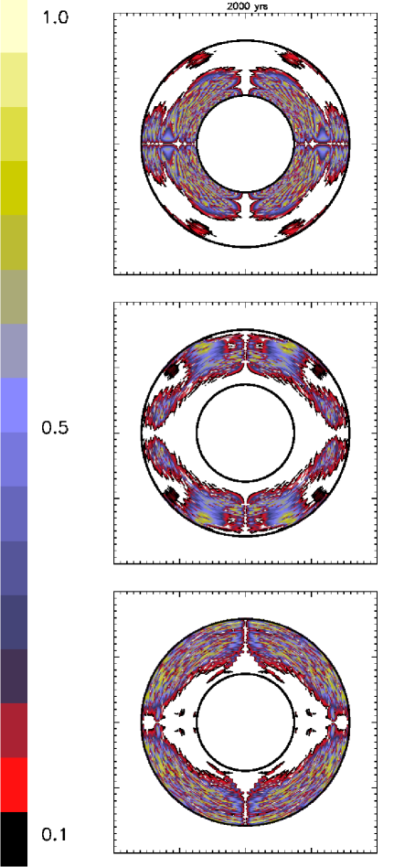
Figure 1.— Snapshot of the deviation of stresses from the previous equilibrium in a typical 2000 yr old magnetar crust. The top, middle and bottom panels show the $(\theta\phi)$, $(r\phi)$, and $(r\theta)$ components of the tensor $M_{ij}-M^{\rm eq}_{ij}$ normalized to the local value of $\sigma_{b}^{\rm max}$. The crustal region has been stretched by a factor of 6 for clarity of visualization. The components of the stress tensor are normalized to the local value of the breaking stress, so that yellow regions are close to the fracture limit.

Fig. 1 shows a snapshot of the deviation of stresses from the previous equilibrium in a typical 2000 yr old magnetar. The yellow regions are close to the breaking limit. Note that at this age the crust has already suffered hundreds of fractures. That history results in the patched appearance. For this run we have fixed $\epsilon=0.9$.

The results about frequency and energy distribution of events are contained in Fig. 2. We remind again that groups of bursts connected to the same fracture are classified as a single outburst in our simulations. We selected three representative periods in a magnetar life, each involving the same total number of events (1000). The first is labeled ”Young” and spans the interval between 400 and 1600 yrs. The second is labeled ”Mid age” and covers the period $\approx 7-10$ kyrs, and the third period is named ”Old” and corresponds to the events recorded from 60 to 100 kyrs. Note that this classification does not pretend to reflect an exact correspondence to SGRs and AXPs, which is just terminology based on historical reasons. Objects that could belong to the first category (young or ”SGR-like”) are SGR 1806-20, SGR 1900+14 and 1E 1547.0-5408; to the Mid Age or ”AXP-like” list could belong SGR 1627-41, SGR 0526-66, SGR 0501+4516, 1E1048.1-5937, or 1E 2259+586 among others; finally, examples of old objects could be SGR 0418+5729, SGR 1833-0832, XTE J1810-197, and PSR J1814-1744.

The first important result is that there is a significant difference in the energetics and recurrence time as the star evolves. This is because the initial evolution of the crustal magnetic field is faster due to the Hall drift, while at late times its has been rearranged into a more quasi-steady state and the evolution proceeds slower. In young magnetars, the typical energies released after each starquake are of the order of $10^{44}$ erg and the typical event rate $\sim$ 1/yr. This does not necessarily imply that a flare will be observed, since this is the energy released in the crust and the mechanism to transfer energy to the surface and magnetosphere may not work in many cases, especially when the fracture occurs in the inner crust. However, in our simulations we observed that more than 95% of the fractures occur in the outer crust, simply because the crust is less strong there, so that we expect a relatively high efficiency of the process. For mid-age objects the energetics is shifted to lower values, a second peak appears at about $10^{41}$ erg, and the waiting time between outbursts increases to a few years. This trend is more pronounced as the object gets older: the recurrence time becomes of the order of tens of years and nearly half the events are low-energy events. The physical reason behind the bimodal distribution is the directionality of stresses. We found that fractures associated to the magnetic stress component $M_{\theta,\phi}$ are more frequent, but they are mostly associated to very low energy events $\mathrel{\hbox to0.0pt{\lower 4.0pt\hbox{\hskip 1.0pt$\sim$}\hss}\raise 1.0pt\hbox{$<$}}10^{41}$ erg. On the other hand, fractures caused by the $M_{r,\phi}$ component are responsible for most of the $E\mathrel{\hbox to0.0pt{\lower 4.0pt\hbox{\hskip 1.0pt$\sim$}\hss}\raise 1.0pt\hbox{$>$}}10^{44}$ erg events. The events associated to large values of $M_{r,\theta}$ span the whole range of energies, but they become very rare after a few kyrs, so that the long-term energy distribution becomes more clearly bimodal. On average, we find that events related to stresses created by the toroidal field are a hundred times more frequent. Our simulations hence predict that giant flares are expected to be less frequent than the less energetic bursts. Indeed, while giant flares have been observed in only 3 objects (once each), bursts have been observed in more than a dozen (often multiple times each).

In Fig. 3 we show the results for the same case, but with the parameter $\epsilon$ varying randomly in the interval [0.95-1] for each event. There is no reason why this parameter must be constant and in fact fracture dynamics cannot be parametrized in a simple form. Nevertheless, with this other study, we can assess the sensitivity of our results to the particular choice of $\epsilon$. The first important remark is that the energy distribution changes and now low-energy events are more frequent than giant-flare-like events even for young magnetars. This choice of values of $\epsilon$ closer to unity reduces the average size of the region implied in the starquake, and selects less energetic events. Interestingly, the bimodal shape of the energy distribution remains qualitatively the same. In the central panel we can see that the age trend discussed in the previous case does not change: the older the object, the longer the average waiting times between two events. The comparison between these two cases indicates that a detailed understanding and modeling of fracture mechanics will be needed before we can make definite, quantitative statements about the energy distribution of starquakes.

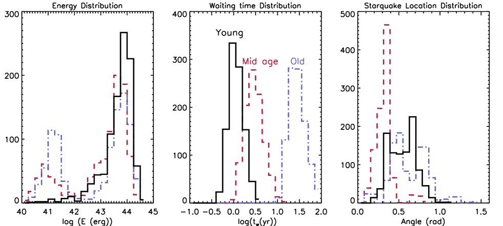
Figure 2.— Outburst properties of an object with initial magnetic field components $B_{p}=8\times 10^{14}$ G and $B_{t}=2\times 10^{15}$ G during three different periods of its lifetime: 400-1600 yr (labeled “Young”), 7-10 kyr (labeled as “Mid age”), and 60-100 kry (labeled as “Old”). We have fixed $\epsilon=0.9$.

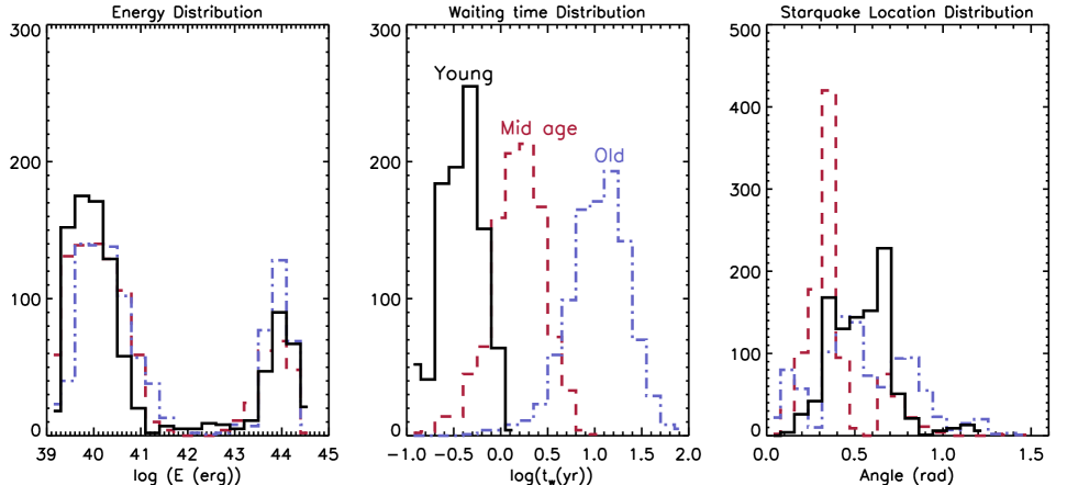
Figure 3.— Same as Fig. 2, but with $\epsilon$ varying randomly in the interval [0.95-1].

It is interesting to compare the general trends predicted by our simulations with the observations. We find that, for a given $B$-field strength and configuration at birth, younger objects are generally more active, both in event frequency and energy of events. Interestingly, this age sequence is also what observations have been hinting at (Kouveliotou, 1999). Our predicted clustering of the energy distribution (around $10^{40}-10^{41}$ and $10^{44}$ erg) is suggestive of the observed dichotomy outbursts/giant flares, with rarer events in between (Kouveliotou et al., 2001; Israel et al., 2008; Mereghetti, 2008). Note that our results predict that middle age objects also show high energy events; interestingly, some of the originally classified AXPs also show SGR-like bursts (Kumar & Safi-harb, 2010). A rigorous comparison with observations cannot be made at this stage, due to the very limited statistics. However, if the secular waiting time distribution of starquakes (which is what we predict) has a similar behaviour to the waiting time distribution of bursts within an outburst, then our results would again match the observations (Cheng et al., 1996; Gogus et al., 2001).

Further connections to the observations can be made by inspection of the right panels of Figs. 2 and 3, where we show the angular distribution of the bursts. While for ”young” and ”old” magnetars there is no clear trend, it is interesting to note that at intermediate age most of the fractures happen at small polar angles. If the polar region is hotter than the equator, our results suggest a correlation between burst location and pulsar phase, which is typical of objects routinely classified as AXPs (Kaspi & Gavriil, 2004; Gavriil et al., 2004). The reason for this particular feature is probably related to the evolution of the internal toroidal field. The Hall drift displaces the internal toroidal field towards the poles in a typical Hall timescale of $10^{3}-10^{4}$ yrs, but after a few Hall timescales the magnetic field is reconfigured in a more stable, steady-state. The characteristic location of starquakes closer to the pole seems to be reflecting this fact. To confirm this point, consistent simulations that include the local heating and the temperature variations produced by the energy release are in progress and will be presented elsewhere.

Finally, we also studied the magnetic evolution of a NS with a lower dipolar magnetic field strength $B_{p}=2\times 10^{14}$ G, and a toroidal component $B_{t}=10^{15}$ G (at birth). We made a longer simulation covering $10^{6}$ yr of this NS and found that, while the energetics is very similar, the event rate is much lower. Even at very early times the typical lapse time between events is about 50-100 yrs. At late times, it becomes larger, ranging from few kyrs to 10 kyrs. The reason why the energetics is similar is simple: the local physical conditions that establish the breaking criteria are the same (Eq. 3), so the elastic energy stored is similar. However, the magnetic field evolves slowly, so it takes more time to bring the system close to the critical conditions. Interestingly, our magneto-thermal evolution model naturally predicts that all NSs, not only magnetars, may show activity in the form of sporadic outbursts or flares. This last case, for which $B_{p}$ becomes $<7\times 10^{12}$ G at an age $>1$  Myr, would be a close representation of the bursting source recently reported by Rea et al. (2010). Other cases studied show similar results, with the particularity that objects with a lower toroidal field are generally less active.

4. Summary

In our study, we have found that there is no real separation among what constitutes the apparently different classes of bursting NSs, and we have identified some key elements that create the variety of observed burst/flare phenomenology. In particular, while what we infer from measurements of $P$ and $\dot{P}$ is only the dipolar component of the $B$-field, both the dipolar component and the hidden toroidal component are similarly important. The lower the field (in either component), the lower is the frequency of starquakes. Although very rare, we find that outbursts can also occur in “low-$B$” pulsars, with $B\sim$ a few $\times 10^{12}$ G. For a given $B$ field at birth, our results show that the age (or the evolutionary stage) is the most relevant feature to determine the different levels of activity in different families of NSs. The same object may behave differently at different times, without in principle having a different nature.

References

- Camilo et al. (2000) Camilo, F., Kaspi, V. M., Lyne, A. G., Manchester, R. N., Bell, J. F., D’Amico, N., Mckay, N. P. F., Crawford, F. 2000, ApJ, 541, 367
- Cheng et al. (1996) Cheng, B., Epstein, R. I., Guyer, R.A., Young, A. C. 1996, Nat., 382, 518
- Chugunov & Horowitz (2010) Chugunov, A. I., Horowitz, C. J. 2010, MNRAS, 407L, 54
- Ciolfi et al. (2010) Ciolfi, R.; Ferrari, V.; Gualtieri, L. 2010, MNRAS, 406, 2540
- Ciolfi et al. (2009) Ciolfi, R.; Ferrari, V.; Gualtieri, L.; Pons, J. A. 2009, MNRAS, 397, 913
- Gavriil et al. (2008) Gavriil, F. P., et al. 2008, Science, 319, 1802
- Gavriil et al. (2004) Gavriil, F. P. , Kaspi, V. M., Woods, P. M. 2004, ApJ, 607, 959
- Gogus et al. (2001) Gogus, E., Kouveliotou, C., Woods, P. M., Thompson, C., Duncan, R. C., Briggs, M. S. 2001, ApJ, 558, 228
- Horowitz & Kadau (2009) Horowitz, C. J., Kadau K. 2009, PRL, 102, 191102
- Horowitz & Hughto (2008) Horowitz, C. J., Hughto, J. 2008, eprint arXiv: 0812.2650
- Israel et al. (2008) Israel, G. et al. 2008, ApJ, 685, 1114
- Kaspi (2010) Kaspi V. M. 2010, Publ. Nat. Acad. Sc. 107, 7147
- Kaspi & Gavriil (2004) Kaspi, V. M., Gavriil F. P. 2004, Nucl. Phys. B, 132, 456
- Kouveliotou (1999) Kouveliotou C. 1999, Proc. Nat. Acad. Sc, 96, 5351
- Kouveliotou et al. (2001) Kouveliotou, C. et al. 2001, ApJL, 558, 47
- Kumar & Safi-harb (2010) Kumar, H. S., Safi-Harb, S. 2010, arXiv:1011.3537
- Lander & Jones (2009) Lander, S.K., Jones, D.I. 2009, MNRAS, 395, 2162
- Mereghetti (2008) Mereghetti, S. 2008, ARA&A, 15, 225
- Pons & Geppert (2007) Pons, J. A., Geppert, U. 2007, A&A, 470, 303
- Pons et al. (2009) Pons, J. A., Miralles J. A. & Geppert U. 2009, A&A, 496, 207
- Rea et al. (2010) Rea, N. et al. 2010, Science, in press, eprint arXiv:1010.2781
- Thompson & Duncan (1995) Thompson, C. & Duncan, R. C. 1995, MNRAS, 275, 255
- Thompson & Duncan (2001) Thompson, C. & Duncan, R. C. 2001, ApJ, 561, 980