Suppression of non-adiabatic losses of molecules from chip-based microtraps

Abstract

Polar molecules in selected quantum states can be guided, decelerated, and trapped using electric fields created by microstructured electrodes on a chip. Here we explore how non-adiabatic transitions between levels in which the molecules are trapped and levels in which the molecules are not trapped can be suppressed. We use ¹²CO and ¹³CO ($a\,^{3}\Pi_{1},v=0$) molecules, prepared in the upper $\Lambda$-doublet component of the $J=1$ rotational level, and study the trap loss as a function of an offset magnetic field. The experimentally observed suppression (enhancement) of the non-adiabatic transitions for ¹²CO (¹³CO) with increasing magnetic field is quantitatively explained.

I Introduction

The manipulation and control of polar molecules above a chip using electric fields produced by microstructured electrodes on the chip surface is a fascinating new research field meek09a . Miniaturization of the electric field structures enables the creation of large field gradients, i.e., large forces and tight potential wells for polar molecules. A fundamental assumption that is made when considering the force imposed on the molecules is that their potential energy only depends on the electric field strength. This is usually a good assumption, since the molecules will reorient themselves and follow the new quantization axis when the field changes direction and their potential energy will change smoothly when the strength of the field changes. This approximation can break down, however, when the quantum state that is used for manipulation couples to another quantum state that is very close in energy. If the energy of the quantum state changes at a rate that is fast compared to the energetic splitting, transitions between these states are likely to occur. For trapped molecules in so-called low-field-seeking states in a static electric potential, such transitions are particularly disastrous when they end up in high-field-seeking states or in states that are only weakly influenced by the electric fields, as this results in a loss of the molecules from the trap. This effect has been investigated previously for ammonia molecules in a Ioffe-Pritchard type electrostatic trap with a variable field minimum. In this macroscopic electrostatic trap, losses due to non-adiabatic transitions were observed on a second time scale when the electric field at the center of the trap was zero; with a non-zero electric field minimum at the center of the trap, these losses could be avoided kirste09 . Non-adiabatic transitions have recently also been investigated in a “conventional”, i.e. macroscopic, Stark decelerator in which electric fields are rapidly switched between two different configurations. There, these transitions have been found to lead to significant losses of molecules when they are in low electric fields wall10 . Similar trap losses will be much more pronounced on a microchip, where the length scales are much shorter and where the electric field vectors change much faster. For atoms in a three-dimensional magnetic quadrupole trap, the trap losses due to spin flip (or Majorana) transitions has been shown to be inversely proportional to the square of the diameter of the atom cloud petrich95 . On atom-chips, where paramagnetic atoms are manipulated above a surface using magnetic fields produced by current carrying wires, trap losses due to Majorana transitions are therefore well-known but can be conveniently prevented by using an offset magnetic field fortagh07 . Due to the geometry of the molecule chip, however, applying a static offset electric field is not possible, and other solutions must be sought.

We have recently demonstrated that metastable CO molecules, laser-prepared in the upper $\Lambda$-doublet component of the $J=1$ level of the $a\,^{3}\Pi_{1},v=0$ state can be guided, decelerated and trapped on a chip. In these experiments, non-adiabatic losses have been observed for ¹²C¹⁶O. In this most abundant carbon monoxide isotopologue, the level that is low-field-seeking becomes degenerate with a level that is only weakly influenced by an electric field when the electric field strength goes to zero. Every time that the trapped molecules pass near the zero field region at the center of a micro-trap, they can make a transition between these levels and thereby be lost from the trap. This degeneracy is lifted in ¹³C¹⁶O due to the hyperfine splitting (the ¹³C nucleus has a nuclear spin $|\vec{I}|=1/2$), and the low-field-seeking levels never come closer than 50 MHz to the non-trappable levels. Therefore, changing from ¹²C¹⁶O to ¹³C¹⁶O (referred to as ¹²CO and ¹³CO from now on) in the experiment greatly improves the efficiency with which the molecules can be guided and decelerated over the surface and enables trapping of the latter molecules in stationary traps on the chip meek09a .

Although it is evident that the 50 MHz splitting between the low-field-seeking and non-trapped levels in ¹³CO is beneficial, it is not a priori clear whether a smaller splitting would already be sufficient or if a still larger splitting would actually be needed to prevent all losses. While the hyperfine splitting in ¹³CO cannot be varied, the degeneracy can be lifted by a variable amount in the normal ¹²CO isotopologue by using a magnetic field. If a magnetic field is applied in addition to the electric field, a splitting can be induced between the low-field-seeking and non-trappable levels of ¹²CO that depends on the strength of the applied magnetic field; in ¹³CO, a magnetic field will actually decrease the splitting between the low-field-seeking and non-trappable levels.

In this paper, we present measurements of the efficiency with which CO molecules are transported over the chip — while they are confined in electric field minima that are traveling at a constant velocity — as a function of magnetic field strength. It is observed that, in the case of ¹²CO, the losses due to non-adiabatic transitions can be completely suppressed in sufficiently high magnetic fields; for ¹³CO on the other hand, the trap losses increase with increasing magnetic field. A theoretical model that can quantitatively explain these observations is also presented. Although the chip is ultimately used to decelerate molecules to a standstill, measuring the efficiency with which molecules are guided at a constant velocity provides a detailed insight into the underlying trap-loss mechanism. Limiting the experiments to constant velocity guiding also makes them more tractable: bringing molecules to a standstill and subsequently detecting them has thus far required five separate phases of acceleration, which greatly complicates efforts to understand the details of the loss mechanism using numerical calculations meek09a . While deceleration at a constant rate to a non-zero final velocity is possible, the measurable signal in such experiments is significantly lower than in constant velocity guiding. Despite the fact that we only measure at constant velocity, we nonetheless apply the model to examine the non-adiabatic losses expected during deceleration. This work thereby furthers the goal of extending trapping on the molecule chip to a wider range of molecules.

II Experimental setup

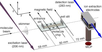
Figure 1: Schematic of the experimental setup. The laser prepared metastable CO molecules are guided over the chip in tubular electric field minima that move at a constant speed of 300 m/s. Above the chip, the molecules are exposed to a time-dependent electric field as well as to a constant magnetic field whose direction is always perpendicular to the electric field. The guided CO molecules are ejected from the chip, ionized via laser induced resonance enhanced multi photon ionization (REMPI), and the CO⁺ ions are mass-selectively detected on a micro-channel plate (MCP) detector. The coordinate system used in the further description is explicitly indicated.

A scheme of the experimental setup is shown in Figure 1. A mixture of 20% CO in krypton is expanded into vacuum from a pulsed valve (General Valve, Series 99), cooled to a temperature of 140 K. In this way, a molecular beam with a mean velocity of 300 m/s and with a full-width-half-maximum spread of the velocity distribution of approximately 50 m/s is produced. This beam passes through two 1 mm diameter skimmers and two differential pumping stages (the valve and first skimmer are not shown in the figure) before entering the chamber in which the molecule chip is mounted. Just in front of the second skimmer, the ground state CO molecules are excited to the upper $\Lambda$-doublet component of the $J=1$ level of the metastable $a\,^{3}\Pi_{1}$, $v=0$ state, using narrow-band pulsed laser radiation around 206 nm (1 mJ in a 5 ns pulse with a bandwidth of about 150 MHz). The metastable CO molecules are subsequently guided in traveling potential wells that move at a constant speed of 300 m/s parallel to the surface of the molecule chip. A uniform magnetic field is applied to the region around the chip using a pair of 30 cm diameter planar coils separated by 23 cm (not shown in the figure). The coils are oriented such that the magnetic field is parallel to the long axis of the chip electrodes, i.e. along the $z$-axis, ensuring that the magnetic field is always perpendicular to the electric field (vide infra). The CO molecules that have been stably transported over the chip will pass through the $50$ µm high exit slit and enter the ionization detection region a short distance further downstream. There, the metastable CO molecules are resonantly excited to selected rotational levels in the $b\,^{3}\Sigma^{+}$, $v^{\prime}=0$ state using pulsed laser radiation at 283 nm (4 mJ in a 5 ns pulse with a 0.2 cm^-1 bandwidth). A second photon from the same laser ionizes the molecules and the parent ions are mass-selectively detected in a compact linear time-of-flight setup using a micro-channel plate (MCP) detector. This detection scheme has been implemented in addition to the Auger detection scheme that we have used in earlier studies meek09a ; meek08 ; meek09 as it is more versatile and can also be applied to detect other molecules. In addition, the detection sensitivity of the ion detector is less affected by the magnetic field than that of the Auger detector.

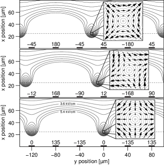
Figure 2: Edge-on view (in the $+z$-direction) of the molecule chip with calculated contour lines of equal electric field strength above the chip, displayed at intervals of 0.45 kV/cm. The three panels correspond to three different times in the harmonic waveform cycle. The position of the electrodes is indicated at the bottom of each panel and the instantaneous values of the applied potentials (in volts) are given. The time difference between adjacent panels is $\frac{1}{12\nu}$, where $\nu$ is the frequency of the harmonic waveforms. From the inset in each panel, it is seen that the electric field at each position relative to the center of the trap rotates clockwise over an angle of $\frac{\pi}{4}$ between adjacent panels.

The molecule chip and its operation principle have been described in detail before meek08 ; meek09 , and only the features that are essential for understanding of the present experiment are discussed here. The active area of the chip consists of an array of 1254 equidistant electrodes, each 10 µm wide and 4 mm long, with a center-to-center distance of 40 µm. An edge-on view of the chip electrodes (with the 4 mm dimension of the electrodes perpendicular to plane of the figure) is shown in Figure 2. The potential (in volts) applied to an electrode at a given moment in time is indicated directly above the electrode; these six potentials are repeated periodically on the electrodes on either side of those drawn here. Because the electrodes are much longer than the period length of the array, the electric field distribution can be regarded as two-dimensional, i.e. the component of the electric field along the $z$-axis can be neglected. This is of importance for the present experiments, because only in this case the applied magnetic field is always perpendicular to the electric field. The calculated contour lines of equal electric field strength in the free space above the chip show electric field minima that are separated by 120 µm, i.e., there are two electric field minima per period, centered about 25 µm above the surface of the chip. By applying sinusoidal waveforms with a frequency $\nu$ to the electrodes, these minima can be translated parallel to the surface with a speed given by $v=120\,\textrm{\textmu m}\cdot\nu$. When these waveforms are perfectly harmonic and have the correct amplitude, offset, and phase, the minima move with a constant velocity at a constant height above the surface, and the shape of the field strength distribution does not change in time. Because an electric field strength minimum acts as a trap for molecules in low-field-seeking states, these fields act as tubular moving traps that can be used to guide the molecules over the surface of the chip. The tubular traps are closed at the end by the fringe fields caused by the neighboring electrodes. Near the ends of the about 4 mm long traps, the electric field will necessarily have a component along the $z$-axis, i.e. parallel to the applied magnetic field. In the present study, where the molecules are guided at 300 m/s over the chip and are therefore on the chip for less than 200 µs, these end-effects are neglected.

The region near an electric field minimum at $(x,y)=(x_{0},y_{0})$ is a quadrupole, with an electric potential given by

$$V=\frac{\alpha}{2}r^{2}\cos(2\phi-\phi_{0})$$ (1)

where $x-x_{0}=r\cos\phi$ and $y-y_{0}=r\sin\phi$. In the current experiment, sinusoidal waveforms with an amplitude of 180 V are applied to the electrodes, yielding a value of $\alpha=0.054\,\textrm{V}/\textrm{\textmu m}^{2}$ meek09 . The resulting electric field is given by

$$\vec{E}=-\alpha r(\cos(\phi_{0}-\phi)\hat{x}+\sin(\phi_{0}-\phi)\hat{y}).$$ (2)

The strength of the electric field, $|\vec{E}|=\alpha r$, depends only on the $r$ coordinate, but the direction of the field vector, $\phi^{\prime}=\phi_{0}-\phi+\pi$, depends on the coordinate $\phi$ and on the phase factor $\phi_{0}$. While the direction of the field vector changes as a result of the motion of the molecule in the quadrupole field (and thus changing $\phi$), the direction of the field at any given position relative to the minimum also rotates when the minimum is translated over the chip. It is seen from the electric field vectors shown in the insets of Figure 2 that the frequency of this rotation is 1.5 times the frequency of the applied waveforms and that the direction of the rotation is clockwise, i.e. the rotation vector points along the positive $z$-axis and $\phi_{0}$ increases linearly in time. To guide the molecules over the chip at 300 m/s, harmonic waveforms with a frequency $\nu$ of 2.5 MHz must be applied, resulting in a rotation frequency of 3.75 MHz.

For CO molecules in the low-field-seeking component of the $J=1$ level, the depth of the tubular traps above the chip is about 60 mK. This implies that CO molecules with a speed of up to 6 m/s relative to the center of the trap can be captured. The oscillation frequency of the molecules in the radial direction of the tubular traps is in the 100–250 kHz range. These parameters are of importance for the non-adiabatic transitions as these determine with which velocity, and how often per second the CO molecules pass by the zero-field region of the traps.

Figure 3: Calculated position of the minimum of an electric field trap with respect to an ideal trap moving at constant velocity during an 800 ns time-interval together with the resulting velocity in the $xy$ plane, using the measured “standard waveforms” (upper row) and “improved waveforms” (lower row) as input.

It turns out that, in the actual experiment, the tubular traps do not move perfectly smoothly over the chip. Due to imperfections in the amplitude, offset and phase of the waveforms that we have used, the tabular traps are jittering at rather high velocities. The motion of the center of the traps relative to the ideal, constant velocity motion can be calculated by measuring the real waveforms applied to the chip and using these to compute the position of the minimum for each point in time. The upper row of Figure 3 shows the motion of a minimum when the waveforms that we will refer to as the “standard waveforms” have been used. The range of this motion extends over $\pm 2$ µm in the $x$ and $y$ coordinates. Although this is considerably smaller than the size of the trapping region, this motion significantly enlarges the effective region in which non-adiabatic transitions can occur. Moreover, the entire path is traced out periodically every $T=2/\nu=800$ ns; because the motion occurs on such a short time scale, the speed with which the trap center moves, and therefore the relative speed with which the molecules encounter the trap center, can be as high as 100 m/s. To improve the waveforms, we inserted an LC filter in the output stage of the amplifiers, thereby reducing the harmonic distortion. The resulting motion using these “improved waveforms” is shown in the lower row of Figure 3. It is seen that not only the range of the motion is now contracted but that also the speed with which the trap center jitters is reduced by about a factor of two.

III Theoretical Model

III.1 Eigenenergies in combined fields

In order to describe the non-adiabatic transitions in CO, we must first derive the energy levels of CO in combined electric and magnetic fields. For this, the field-free Hamiltonian is expanded with Stark and Zeeman contributions, i.e.,

$$\hat{H}=\hat{H}_{\Lambda,\textrm{hfs}}+\hat{H}_{S}+\hat{H}_{Z}.$$ (3)

Here, $\hat{H}_{\Lambda,\textrm{hfs}}$ describes the $\Lambda$-doubling of the $a\,^{3}\Pi_{1}$, $v=0$, $J=1$ level for either ¹²CO or ¹³CO and also includes the hyperfine splitting of each $\Lambda$ component into $F=1/2$ and $F=3/2$ hyperfine sublevels for ¹³CO; $\hat{H}_{S}=-\hat{\vec{\mu}}_{E}\cdot\vec{E}$ is the Stark interaction Hamiltonian and $\hat{H}_{Z}=-\hat{\vec{\mu}}\cdot\vec{B}$ is the Zeeman interaction Hamiltonian, where $\hat{\vec{\mu}}_{E}$ and $\hat{\vec{\mu}}$ are the electric and magnetic dipole moment operators, respectively, and $\vec{E}$ and $\vec{B}$ are the (time-dependent) electric and magnetic field vectors.

The spectroscopic parameters of the $a\,^{3}\Pi_{1}$, $v=0$ state of CO that are used in the field-free Hamiltonian are given elsewhere meek10 ; wicke72 ; gammon71 ; carballo88 ; yamamoto88 ; wada00 ; field72 ; warnerphd . The $\Lambda$-doublet splitting between the positive parity component (upper) and the negative parity component (lower) of the $J=1$ level is about 400 MHz while the hyperfine splitting of each parity level of ¹³CO into $F=1/2$ (lower) and $F=3/2$ (upper) sublevels is about one order of magnitude smaller. The body-fixed electric dipole moment $\mu_{E}=|\vec{\mu}_{E}|$ in the electronically excited metastable state is 1.3745 Debye for both ¹²CO and ¹³CO wicke72 ; gammon71 . The magnetic moment of the molecule can be expressed as $\hat{\vec{\mu}}=-\mu_{B}\,(g_{L}\cdot\hat{\vec{L}}+g_{S}\cdot\hat{\vec{S}})$, where $\mu_{B}$ is the Bohr magneton, $\hat{\vec{L}}$ is the electron orbital angular momentum operator, $\hat{\vec{S}}$ is the electron spin operator, and where the magnetic $g$-factors are fixed at the values of the bare electron, $g_{L}=1.0$ and $g_{S}=2.0023$.

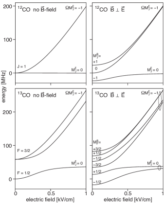
Figure 4: Energy of the upper (positive parity) $\Lambda$-doublet component of the $J=1$ level of ¹²CO (upper panels) and ¹³CO (lower panels) in the electronically excited $a\,^{3}\Pi_{1}$, $v=0$ state as a function of the electric field strength, without (left column) and with (right column) an offset magnetic field. The strength of the magnetic field is 50 Gauss and its direction is perpendicular to the direction of the electric field. The labeling of the energy levels is explained in the text.

A detailed description of the formalism used to calculate the eigenenergies of the various components of the $J=1$ level in the $a\,^{3}\Pi_{1}$, $v=0$ state of both ¹²CO and ¹³CO in combined electric and magnetic fields is presented in the Appendix. The formalism has been set up for mutually orthogonal static electric and magnetic fields. As will be discussed below, this is also adequate to treat the actual situation, in which the electric field rotates with a constant frequency in a plane perpendicular to the magnetic field. In Figure 4 we only show the outcome of these calculations in the form of plots of the energy levels for the upper $\Lambda$-doublet component of ¹²CO and ¹³CO as a function of electric field strength in the absence (left column) or in the presence of a 50 Gauss magnetic field (right column). At low electric field strengths, the Stark shift is quadratic, but as the electric field strength increases and $|H_{S}|$ becomes much larger than $|H_{\Lambda,\textrm{hfs}}|$ and $|H_{Z}|$, the Stark energy shows a linear dependence on the electric field strength, i.e. $\Delta E_{S}\propto-\Omega M_{J}^{E}\mu_{E}E$, and the product of the projection of the electronic angular momentum along the internuclear axis $\Omega$ and the projection $M_{J}^{E}$ of the angular momentum $\hat{\vec{J}}$ on the electric field vector $\vec{E}$ becomes an approximately good quantum number. If a weak magnetic field such as that present in the experiment is applied in the absence of an electric field, each of the zero-field levels splits into $(2J+1)$ (or in $(2F+1)$) separate levels based on their $M_{J}^{B}$ (or $M_{F}^{B}$) quantum number. The Zeeman energy is linear in magnetic field and can be calculated using first order perturbation theory as $\Delta E_{Z}\approx\mu_{\textrm{eff}}MB$ where $M=M_{J}^{B}$ (or $M_{F}^{B}$) and $\mu_{\textrm{eff}}\sim\mu_{B}$ describes the effective magnetic moment of a particular parity and, in the case of ¹³CO, particular $F$ component. When a strong electric field is applied to the molecule in addition to the magnetic field, such that $|H_{S}|\gg|H_{\Lambda,\textrm{hfs}}|,|H_{Z}|$, the energy levels can again be characterized with the approximately good quantum number $\Omega M_{J}^{E}$ and show a linear Stark shift.

The behavior of the eigenenergies in static electric and magnetic fields is quite instructive in describing the non-adiabatic transitions — and thus losses — of molecules from the low-field-seeking states ($\Omega M_{J}^{E}=-1$) to non-trappable ($M_{J}^{E}=0$) states. Near the edge of the trap, where the electric field is as high as 4.2 kV/cm, the Stark effect provides an energy gap of about $U_{\textrm{trap}}=60\,\textrm{mK}\simeq 1.3\,\textrm{GHz}$ between low-field-seeking states and non-trappable states. Since this is much larger than both the frequency of the motion of the molecules in the traps and the frequency of the applied waveforms, non-adiabatic losses will not occur near the edge of the trap. In the vicinity of the trap center, however, this argument no longer holds, and the eigenfunctions can change from $M_{J}^{E}$-type wavefunctions to $M_{J}^{B}$-type (or $M_{F}^{B}$-type) at a rate faster than the energy gap $E_{\textrm{gap}}$ in that region. In the case of a ¹²CO molecule, the energy gap at the center of the trap goes to zero in the absence of a magnetic field. If a molecule in a low-field-seeking state flies near the trap center with a velocity $v$ high enough, or with a distance of closest approach $b$ small enough, that the corresponding interaction time with the trap center $\tau=b/v$ no longer fulfills the adiabaticity condition, i.e. when the condition $E_{\textrm{gap}}\gg h/\tau$ no longer holds, then the probability of transitions to non-trappable states can become significant. In the absence of a magnetic field, ¹³CO molecules are much safer from such non-adiabatic losses due to the energy gap of 50 MHz between the $F=3/2$ level (which becomes low-field-seeking in an electric field) and the $F=1/2$ level (which correlates with non-trappable $M_{J}^{E}=0$ states).

III.2 Calculating rates for non-adiabatic transitions

The basic idea underlying the calculation of the non-adiabatic losses for the molecules in low-field-seeking states is that, since the transitions to non-trappable states happen primarily as the molecules pass the zero field region at the center of a microtrap, the overall loss probability can be estimated by first calculating the loss probability in a single pass. For simplicity, the trajectory of the CO molecules is assumed to have a constant velocity; this is reasonable, since the forces on the molecules approach zero at the center of the trap due to the $\Lambda$-doubling. The transition probability $P_{i,j}(v,B,b)$ of a molecule making a transition from a low-field-seeking state $i$ to a non-trappable state $j$ for a single pass by the trap center depends on the speed of the molecule relative to the center of the trap $v$, on the strength of the magnetic field $B$, and on the distance of closest approach $b$. Due to the rotation of the electric field, there is a difference between positive and negative values of $b$, which is why we do not refer to it as an “impact parameter” here.

To calculate the probability $P_{i,j}(v,B,b)$, the time-dependent Schrödinger equation, which describes the evolution of the quantum states, must be solved:

$$i\hbar\frac{\partial\psi}{\partial t}=\hat{H}\psi.$$ (4)

This equation is solved numerically as an initial value problem on a set of coupled first-order ordinary differential equations using the basis vectors given in the Appendix. The Hamiltonian $\hat{H}$ depends on the electric field vector $\vec{E}$, which, for a molecule moving in the trap, is a function of both position $\vec{r}(t)$ (due to the inhomogeneous field distribution) and time $t$ (due to the rotation of the field vectors relative to the trap center), as discussed in Section II. The time dependent Hamiltonian that the molecule experiences is calculated by assuming a position in time given by $r(t)=(vt-x_{\textrm{init}})\hat{x}+b\hat{y}$, which corresponds to the molecule moving with a constant velocity $v$ and approaching the trap center with a minimum distance $b$. The variable $x_{\textrm{init}}$ must be chosen such that the initial position $r(0)=-x_{\textrm{init}}\hat{x}+b\hat{y}$ is sufficiently far from the center such that at $r(0)$ the adiabaticity condition is still satisfied.

The initial state of the molecule could be chosen as a low-field-seeking eigenstate of the instantaneous Hamiltonian at the initial position and time. If the electric field vector is rotating, however, the wavefunction of the molecule will immediately accumulate amplitude in other quantum states, even if the magnitude of the electric field is constant. The amplitude that appears in other states will only be negligible if the energy splitting between them and the initial state is much larger than the rotation frequency. Alternatively, one can choose an initial state that is a stationary state in the rotating system, as will be discussed below. The calculation of the transition probability as the molecule flies past the field minimum can then be started at lower fields, i.e. with a smaller value of $x_{\textrm{init}}$.

In the current system, the magnetic field vector is oriented along the $\hat{z}$ axis and the electric field vector lies in the $xy$ plane. If the angle of the electric field vector with respect to the $+\hat{x}$ axis (toward the $+\hat{y}$ axis) is given by $\phi^{\prime}$, the Hamiltonian of the molecule can be computed by rotating the physical system around the $\hat{z}$ axis through an angle $-\phi^{\prime}$, operating on it with a Hamiltonian $\hat{H}^{\prime}$ which corresponds to a system with the same magnetic field vector and in which the electric field has the same magnitude but is directed along the $+\hat{x}$ axis, and then rotating the physical system back through an angle $\phi^{\prime}$. In operator form, this can be written as

$$\hat{H}=e^{-i\hat{F}_{z}\phi^{\prime}}\hat{H}^{\prime}e^{i\hat{F}_{z}\phi^{\prime}}$$ (5)

where $\hat{F}_{z}$ is the total angular momentum of the molecule along the $\hat{z}$ axis. Using this form of $\hat{H}$, equation (4) can be rewritten as

$$i\hbar\frac{\partial\psi_{Q}}{\partial t}=\Bigl{(}\hat{H}^{\prime}-\hat{F}_{z}\hbar\frac{\partial\phi^{\prime}}{\partial t}\Bigr{)}\psi_{Q}$$ (6)

where $\psi_{Q}=e^{i\hat{F}_{z}\phi^{\prime}}\psi$. This equation has the same form as equation (4) and can be solved in the same way as the time independent Schrödinger equation if the magnetic field is constant, the electric field strength is constant, and the electric field vector rotates at a constant frequency. The eigenvalues that result are called “quasienergies” and $\hat{H}_{Q}=\hat{H}^{\prime}-\hat{F}_{z}\hbar\frac{\partial\phi^{\prime}}{\partial t}$ is the quasienergy Hamiltonian zeldovich67 ; ritus67 . A similar approach has been used in the recent work by Wall et al. wall10 .

In section II it was shown that the angle of the electric field in the $xy$ plane $\phi^{\prime}=\phi_{0}-\phi+\pi$ contains contributions from both the angular coordinate of the molecule with respect to the trap center $\phi$ and a phase that results from the constant rotation of the field vectors as the traps move over the chip $\phi_{0}=2\pi\frac{3\nu}{2}\,t$. Because $\phi_{0}$ increases linearly in time, the contribution of $\phi_{0}$ to the quasienergy Hamiltonian is time independent, having the form $-h\frac{3\nu}{2}\hat{F}_{z}$. This operator is diagonal in the basis sets used for both ¹²CO and ¹³CO, and in the case of ¹²CO, it is exactly equivalent to the Zeeman interaction for each energy eigenstate. As the rotation frequency $\frac{3\nu}{2}$ is 3.75 MHz when the molecules are guided with 300 m/s over the chip, its contribution to the quasienergy Hamiltonian is equivalent to a magnetic field of about $-8$ Gauss. It should be understood, however, that we are not dealing with a real magnetic field produced by the rotating electric field here; the effect of a rotating coordinate system merely produces a shift to the quasienergies that resembles the Zeeman Hamiltonian but that does not depend on the magnetic moment. In the case of ¹³CO, the rotation frequency is not equivalent to a Zeeman interaction since, as stated in the definition of $\hat{\vec{\mu}}$, the gyromagnetic factors of the orbital angular momentum and the electron spin are different.

For the subsequent calculations, the quasienergy eigenvector instead of the normal Hamiltonian eigenvector is chosen as the initial state. After choosing an initial state $i$ at the position $r(0)=-x_{\textrm{init}}\hat{x}+b\hat{y}$, the quasienergy vector is propagated in time using equation (6) until the molecule reaches the position $r(t_{\textrm{final}})=x_{\textrm{init}}\hat{x}+b\hat{y}$. The final state is then expressed in terms of quasienergy eigenvectors at the final position and time, and the probability of the molecule ending up in a state $j$, $P_{i,j}(v,B,b)$, is calculated. For all calculations, the population is assumed to be initially distributed equally over all low-field-seeking levels, two for ¹²CO and four for ¹³CO. In ¹²CO, the calculation of $P_{i,j}(v,B,b)$ only needs to be carried out for the initial state $i$ corresponding to the $M_{J}^{B}=+1$ low-field-seeking level, since the $M_{J}^{B}=0$ low-field-seeking level is completely stable against non-adiabatic transitions (see the Appendix). For ¹³CO, none of the four low-field-seeking levels is stable against non-adiabatic transitions at all magnetic fields, so $P_{i,j}(v,B,b)$ must be calculated for each initial level $i$.

In the end, we are interested in the probability $T(B)$ of a molecule remaining in a low-field-seeking state for the duration of its time in the microtrap, as this is the quantity that is measured in the experiment. For ¹²CO molecules in the ideal case, i.e. when the electric field is perfectly perpendicular to the magnetic field and the traps move perfectly smoothly over the chip, the survival probability for a single molecule in a single state is given by the product of its survival probabilities after each individual encounter with the trap center. The overall transmission probability $T(B)$ is then calculated by averaging this over both low-field-seeking states and over $N$ molecules.

$$\begin{split}T(B)=\frac{1}{N}\sum_{n=1}^{N}\Biggl{[}&\frac{1}{2}\prod_{k=1}^{K}P_{M_{J}^{B}=0,M_{J}^{B}=0}(v_{n,k},B,b_{n,k})+\\ &\frac{1}{2}\prod_{k=1}^{K}P_{M_{J}^{B}=+1,M_{J}^{B}=+1}(v_{n,k},B,b_{n,k})\Biggr{]}\end{split}$$ (7)

The total number of passes $K$ of each molecule and the speed $v_{n,k}$ and closest approach distance $b_{n,k}$ of the $k$th pass of the $n$th molecule are determined using simulations of the classical trajectory of a molecule in the trap, as described elsewhere meek09 . Since the $M_{J}^{B}=0$ state is completely stable, $P_{M_{J}^{B}=0,M_{J}^{B}=0}(v_{n,k},B,b_{n,k})=1$, and the transmission probability $T(B)$ in the ideal case can never be less than $1/2$. For ¹³CO, calculating $T(B)$ is somewhat more complicated, since the $F=3/2,M_{F}^{B}=+3/2$ low-field-seeking level and the $F=3/2,M_{F}^{B}=-1/2$ low-field-seeking level are coupled, as are the $F=3/2,M_{F}^{B}=+1/2$ and $F=3/2,M_{F}^{B}=-3/2$ levels. During each encounter with the trap center, a molecule in a particular low-field-seeking state can transition not only to a non-trappable state but also to one other low-field-seeking state. To calculate the transmission probability of a single ¹³CO molecule, the population in each low-field-seeking state after an encounter with the trap center is computed based on the population distribution before the encounter, and the total population still in a low-field-seeking state after the last pass is recorded. As in ¹²CO, $T(B)$ is obtained by averaging the result of this calculation over a large number of molecules.

To accurately describe the experimental data, the theoretical calculations must be extended to include the jittering motion of the traps and the nonperpendicularity of the electric and magnetic fields. The jittering motion is accounted for by including the full motion of the center of the trap as shown in Figure 3 in the calculation of the transition probability $P_{i,j}(v,B,b,t,\phi)$. As in the ideal case, the transition probability depends on speed $v$, magnetic field $B$, and closest approach distance $b$ (although this distance is now defined relative to the average position of the minimum instead of the actual position). Additionally, the transition probability now also depends on the time $t$ at which the molecule arrives relative to the jittering cycle and the direction $\phi$ from which it comes. If the electric and magnetic fields are not exactly perpendicular, low-field-seeking states that are normally decoupled can mix. In ¹²CO, the $M_{J}^{B}=0$ and $M_{J}^{B}=+1$ states, which converge asymptotically at high electric fields, then become coupled. As a result, the population can partially redistribute between these two levels while the molecule is in a region of high electric field between successive encounters with the trap center. To account for this effect, it is assumed in the calculations that, after each encounter with the trap center, a molecule’s population $n$ in each of these two low-field-seeking states is redistributed such that

$$n^{\prime}_{M_{J}^{B}=+1} =(1-m)n_{M_{J}^{B}=+1}+mn_{M_{J}^{B}=0}$$ (8)

$$n^{\prime}_{M_{J}^{B}=0} =(1-m)n_{M_{J}^{B}=0}+mn_{M_{J}^{B}=+1}$$ (9)

where $n^{\prime}$ is the new population distribution. The parameter $m$ describes the degree of the redistribution; at the extremes, a value of $0$ indicates that no redistribution occurs while a value of $1/2$ corresponds to complete redistribution. Its exact value is difficult to predict and should actually depend on the trajectory of the molecule. For simplicity, $m$ is determined by fitting it to the data; note that this is the only fitting parameter used. For ¹³CO, remixing can occur at high electric fields between the $F=3/2,M_{F}^{B}=-3/2$ and the $F=3/2,M_{F}^{B}=-1/2$ levels and also between the $F=3/2,M_{F}^{B}=+1/2$ and the $F=3/2,M_{F}^{B}=+3/2$ levels. The remixing coefficient $m$ can be different for each of these pairs of levels, and thus for ¹³CO, two fitting parameters are necessary.

IV Experimental results

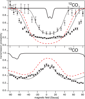
Figure 5: Measured signal of ¹²CO (upper panel) and ¹³CO (lower panel) molecules guided over the chip at 300 m/s as a function of the magnetic field. The vertical scaling of the individual data sets is described in the text. Measurements have been performed using the “standard waveforms” (filled circles) for both ¹²CO and ¹³CO; for ¹²CO, measurements with the “improved waveforms” (open circles) are shown as well. The simulated curves of the transmission probability $T(B)$ are shown as solid curves that overlay the data points. The thick solid curves in the upper and in the lower panel result from the theoretical model for the ideal case. The red dashed curves show the prediction of the theoretical model for the survival probability of molecules decelerated from 300 m/s to zero velocity in 250 µs.

To measure the effectiveness of the magnetic field at suppressing non-adiabatic losses, metastable CO molecules are guided over the full length of the chip at a constant velocity of 300 m/s and are subsequently detected using laser ionization. Measurements are carried out for both positive and negative magnetic fields, where the direction of positive magnetic field coincides with the $+\hat{z}$-axis (see Figure 1). To compensate for long term drifts in the intensity of the molecular beam, the parent ion signal is measured with the magnetic field on and with the magnetic field off, and the ratio between these two measurements is recorded. In Figure 5, the thus recorded relative number of ¹²CO (upper panel) and ¹³CO (lower panel) molecules that are guided over the chip is shown as a function of the applied magnetic field. Both the measurements with the “standard waveforms” and with the “improved waveforms” are shown in the upper panel.

It is clear from the data shown in Figure 5 that, as the magnetic field strength increases, the number of ¹²CO molecules reaching the detector increases. This is as expected because the splitting between the low-field-seeking levels of ¹²CO and the non-trappable level increases with the magnetic field strength, thereby increasingly suppressing non-adiabatic losses. The measurements with the “improved waveforms” show that at magnetic fields more negative than $-40$ Gauss and more positive than $+50$ Gauss, the number of guided molecules becomes constant, indicating that all non-adiabatic losses are suppressed under these conditions. The data have been scaled vertically such that the saturation observed at high magnetic field strengths corresponds to a transmission of unity. The ratio between the signal at high magnetic field and low magnetic field is smaller than when the “standard waveforms” are used, implying that the “improved waveforms” also reduce the losses without a magnetic field. The number of ¹³CO molecules reaching the ionization detector, on the other hand, is seen to decrease as a function of magnetic field. The vertical scale in this case is based on the results of the theoretical calculations at low magnetic field strengths (vide infra). The lower panels of Figure 4 show that the $M_{F}^{B}=+1/2$ level of the non-trappable $F=1/2$ state increases in energy in a magnetic field, while the $M_{F}^{B}=-3/2$ and $M_{F}^{B}=-1/2$ levels of the low-field-seeking $F=3/2$ state are at the same time lowered in energy. This reduction of the energy gap between the low-field-seeking and non-trappable levels enhances the non-adiabatic losses. Both the ¹²CO and ¹³CO data are slightly asymmetric for positive and negative magnetic fields. The data for ¹²CO indeed seem to be symmetric around a magnetic field of about $+8$ Gauss, as expected from the theoretical model.

The results of the theoretical models are shown as solid curves in Figure 5 as well. The thick solid curves in the upper and in the lower panel result from the theoretical model for the ideal case, i.e. when the jittering of the traps would be absent and no remixing would occur between decoupled states. The width of the theoretically predicted transmission minimum for ¹²CO around $+8$ Gauss depends sensitively on the relative velocity between the CO molecule and the center of the trap as they pass, and gets larger with increasing velocities. In the case of ¹³CO, two narrow transmission minima are expected around $-65$ Gauss and $+90$ Gauss, corresponding to fields at which the the $F=1/2,M_{F}^{B}=+1/2$ and $F=3/2,M_{F}^{B}=-3/2$ levels cross, and between these two minima, no losses are expected. As in ¹²CO, the width of the transmission minima increases as the relative velocity between the molecules and the trap center increases. It is clear from the comparison of these theoretical curves with the experimental data, that the observed measurements can not be quantitatively explained if the traps are assumed to move smoothly over the chip; the jittering of the traps must be taken into account.

The transmission probabilities calculated for the case in which the jittering is explicitly taken into account are seen to almost quantitatively agree with the measurements. In particular the theoretical curves reproduce the asymmetry between the intensity of the guided ¹²CO molecules at positive and negative magnetic fields as well as the narrowing of the profiles when the waveforms are improved. In the calculations for ¹²CO, a partial redistribution after each pass of 18% ($m=0.09$) has been assumed for the “standard waveforms” and 12% ($m=0.06$) for the “improved waveforms”. It can not be excluded that the jittering of the traps was still slightly more severe during the actual experiments than shown for the “standard waveforms” in Figure 3, which would explain the experimentally observed additional broadening for that case. In the ¹³CO calculations, the best agreement with the experimental data was found when assuming no remixing between the $M_{F}^{B}=+3/2$ and the $M_{F}^{B}=+1/2$ levels, and 30% remixing ($m=0.15$) between the $M_{F}^{B}=-1/2$ and the $M_{F}^{B}=-3/2$ level. The maximum transmission at about $+10$ Gauss is not sensitive to the remixing coefficients, since the transition probability for each of the low-field-seeking states is about the same in this region. It can be reliably inferred from the theoretical calculations that, even at low magnetic fields, about $1/3$ of the ¹³CO molecules are lost to non-adiabatic transitions while being guided over the chip. Based on this, the ¹³CO data shown in the lower panel of Figure 5 have been scaled vertically such that the transmission at zero magnetic field is 2/3.

The theoretical model used to explain the guiding data can also be applied to predict the non-adiabatic losses that are expected to occur during linear deceleration. The red dashed curves in the upper (lower) panel of Figure 5 show the survival probability of ¹²CO (¹³CO) molecules decelerated from 300 m/s to zero velocity in 250 µs. In these calculations, it is assumed that the jittering motion at 300 m/s is that of the “standard waveforms”. The velocity of the jittering motion is assumed to be proportional to the frequency of the applied waveforms while the latter is reduced from 2.5 MHz to zero. For ¹²CO at low magnetic fields, the survival probability during deceleration is only 1/4 of the survival probability of ¹²CO guided at a constant velocity of 300 m/s. The magnetic field needed to suppress losses is smaller, however. While the survival probability for guiding is symmetric around a magnetic field of +8 Gauss, the symmetry point for deceleration is shifted closer to zero field, to +4 Gauss, due to the lower rotation frequency of the electric field vectors in the trap at lower velocities. For ¹³CO, the model predicts that the transmission probability during deceleration is larger than for guiding at all magnetic field strengths.

The differences in transmission probability between guiding and deceleration can result from various effects that either enhance or suppress losses as the deceleration of the trap increases. The smaller spatial acceptance of a strongly accelerated trap results in a larger fraction of the trapped cloud being in the jittering region at any given time, which enhances the losses during deceleration meek09 . Losses are also enhanced due to the molecules spending a longer time on the chip. On the other hand, since the average velocity of a decelerating trap is lower than that of a trap at constant velocity, the velocity of the jittering motion is reduced, suppressing non-adiabatic losses. While it is difficult to predict through simple arguments the relative importance of these effects, the outcome of the calculations is corroborated by previous measurements at zero magnetic field, in which it was shown that ¹³CO molecules can be decelerated to a standstill while ¹²CO molecules are rapidly lost with increasing deceleration meek09a .

V Conclusions

In this paper we have studied the losses due to non-adiabatic transitions in metastable CO molecules — laser-prepared in the upper $\Lambda$-doublet component of the $J=1$ level in the $a\,^{3}\Pi_{1}$, $v=0$ state — guided at a constant velocity in microtraps over a chip. Transitions between levels in which the molecules are trapped and levels in which the molecules are not trapped can be suppressed (enhanced) when the energetic splitting between these levels is increased (decreased) by the application of a static magnetic field. For a quantitative understanding of this effect, the energy level structure of ¹²CO and ¹³CO molecules in combined magnetic and electric fields has been analyzed in detail. When the CO molecules are guided over the chip, they are in an electric field that rotates with a constant frequency; the direction of the externally applied magnetic field is perpendicular to the plane of the electric field. The probability with which either ¹²CO or ¹³CO molecules are transmitted over the chip, i.e. the probability that the molecules stay in a trapped level for the complete duration of the flight over the chip, has been measured as a function of the magnetic field. The observed transmission probability can be quantitatively explained.

To reduce trap losses in future experiments, it will be important to improve the applied waveforms. This will not only reduce losses due to non-adiabatic transitions caused by the jittering, but it will also reduce losses due to mechanical heating. Mechanical losses might also have been present in the current experiment, but because the measurements always compared the guiding efficiency with magnetic field on and off, we have not been sensitive to these losses. Alternatively, it might be possible to avoid the need for improved waveforms by moving the minimum on an orbit that is much larger than the amplitude of the jittering motion, creating a large region around the effective trap center through which the minimum never passes. Such a trap, known as a time orbiting potential (TOP) trap, prevents non-adiabatic losses but is much shallower than a static trap petrich95 .

The intrinsic difficulties with making the waveforms required for the experiments discussed here should be stressed; with present day technology these waveforms can hardly be made better than we have them now, in particular because, in order to bring molecules to a standstill, we want to be able to rapidly chirp the frequency down from 2.5 MHz to zero. While the LC filter used to produce the “improved waveforms” reduces the total harmonic distortion of the amplitudes from 7% to 3%, it also makes producing a constant amplitude frequency chirp more complicated. We are nevertheless optimistic that the jittering can be reduced by another factor of two to three relative to the best waveforms that we have used so far. In the case of ¹²CO, for instance, a magnetic field of 10 Gauss, applied in the right direction, would then already completely avoid losses due to non-adiabatic transitions. With the present waveforms, trap losses can only be avoided when the applied magnetic fields are made sufficiently high. One should realize that there is an upper limit to these fields, however, as at some point transitions to the lower $\Lambda$-doublet components can be induced, opening up a new loss-channel.

The extreme sensitivity to the details of the applied voltages results from the fact that the electric field minima above the chip originate from the vectorial cancellation of rather large electric field terms. Design studies are in progress to find an electrode geometry that is less sensitive to imperfections in the applied waveforms. A modified electrode geometry is also required to avoid trap losses at the ends of the tubular traps. Although the ends are closed in the present geometry by the fringe fields of adjacent electrodes, the electric field near the ends has components along the long axis of the trap, presumably leading to non-adiabatic losses even in the presence of the offset magnetic field.

*

Appendix A The $\boldsymbol{a\,^{3}\Pi_{1}}$, $\boldsymbol{v=0}$, $\boldsymbol{J=1}$ Hamiltonian

In this Appendix, the formalism that has been used to calculate the energies of the $M$-components of the $J=1$ level in the $a\,^{3}\Pi_{1}$, $v=0$ state of both ¹²CO and ¹³CO in combined, but mutually orthogonal, static electric and magnetic fields is presented. In the coordinate system used here, the magnetic field vector is oriented along the $\hat{z}$ axis and the electric field vector is in the $xy$ plane. In this case, the molecular Hamiltonian is invariant under reflection in the $xy$-plane. It is thus possible to separate the basis states into two uncoupled sets, consisting of wavefunctions that are either symmetric or antisymmetric under reflection in the $xy$-plane, thereby reducing the computational complexity. The magnetic field can only couple states of the same parity and the same $M_{F}^{B}$ quantum number, where $M_{F}^{B}$ is the projection of the total angular momentum including nuclear spin along the $+\hat{z}$ axis. In the case of ¹²CO, there is no hyperfine interaction and thus $F\equiv J$ and $M_{F}^{B}\equiv M_{J}^{B}$. As the electric field vector lies in the plane perpendicular to the quantization axis it can only couple states of opposite parity with $M_{F}^{B}$ differing by $\pm 1$. The two resulting sets of uncoupled basis states for ¹²CO are given by:

1. M${}_{J}^{B}=-1,\pm$

2. M${}_{J}^{B}=0,\mp$

3. M${}_{J}^{B}=1;\pm$

The $+$ and $-$ sign at the end describe the parity of the basis state. All states with the upper (lower) sign belong to one set. For ¹³CO there are two sets containing six basis states each:

1. $F=3/2,M_{F}^{B}=-3/2,\pm$

2. $F=1/2,M_{F}^{B}=-1/2,\mp$

3. $F=3/2,M_{F}^{B}=-1/2,\mp$

4. $F=1/2,M_{F}^{B}=1/2,\pm$

5. $F=3/2,M_{F}^{B}=1/2,\pm$

6. $F=3/2,M_{F}^{B}=3/2,\mp$

Again, all states with the upper (lower) parity belong to one set.

Based on this formalism and using the zero-field spectroscopic parameters and matrix elements given in references meek10 ; wicke72 ; gammon71 ; carballo88 ; yamamoto88 ; wada00 ; field72 ; warnerphd , the corresponding Hamiltonian matrices can be calculated. Without loss of generality, the electric field vector is taken to be oriented along the $\hat{x}$ axis, i.e. $\vec{E}=E\hat{x}$. The Hamiltonian matrices for other orientations of the electric field vector in the $xy$ plane can be computed using the unitary transformation given in equation (5); the matrices given here correspond to $\hat{H}^{\prime}$ in this equation. The origin of the energy scale for each isotopologue is defined to be the lowest energy field-free state in the upper $\Lambda$-doublet component, as shown in Figure 4.

For ¹²CO, the matrices $\hat{H}_{\textrm{upper}}$ and $\hat{H}_{\textrm{lower}}$ for the set of basis states with the upper and lower parity, respectively, are given by:

$$\hat{H}_{\textrm{upper}}=\begin{pmatrix}-R_{1}&S&0\\ S&-\Lambda&S\\ 0&S&R_{1}\\ \end{pmatrix}$$ (10)

and

$$\hat{H}_{\textrm{lower}}=\begin{pmatrix}-\Lambda-R_{2}&S&0\\ S&0&S\\ 0&S&-\Lambda+R_{2}\\ \end{pmatrix}$$ (11)

where $\Lambda=394.066~{}\textrm{MHz}$
$R_{1}=\langle 1,+|\hat{H}_{Z}|1,+\rangle=0.3332\mu_{B}B$
$R_{2}=\langle 1,-|\hat{H}_{Z}|1,-\rangle=0.3406\mu_{B}B$
$S=\langle 0,+|\hat{H}_{S}|1,-\rangle=0.3513\mu_{E}E$,
and the bra and ket vectors have the form $|M_{J}^{B},\textrm{parity}\rangle$. It is clear from these matrices, that the energy level labeled as $M_{J}^{B}$=0 in the case of ¹²CO (upper right panel of Figure 4) is only directly coupled to the $M_{J}^{B}$=$\pm$1 levels of the lower $\Lambda$-doublet component and that there is no direct coupling to the nearby $M_{J}^{B}$=$\pm$1 levels of the upper $\Lambda$-doublet component. Provided that the electric and magnetic fields are exactly perpendicular, this $M_{J}^{B}$=0 level is therefore stable against non-adiabatic transitions.

For ¹³CO, the corresponding matrices for the sets of basis states with the upper and lower parity are given by:

$$\hat{H}_{\textrm{upper}}=\begin{pmatrix}E_{1}-3R_{5}&\sqrt{3}S_{3}&\frac{\sqrt{3}}{2}S_{4}&0&0&0\\ \sqrt{3}S_{3}&-E_{3}-R_{2}&R_{4}&S_{1}&-S_{3}&0\\ \frac{\sqrt{3}}{2}S_{4}&R_{4}&-E_{2}-R_{6}&S_{2}&S_{4}&0\\ 0&S_{1}&S_{2}&R_{1}&R_{3}&-\sqrt{3}S_{2}\\ 0&-S_{3}&S_{4}&R_{3}&E_{1}+R_{5}&\frac{\sqrt{3}}{2}S_{4}\\ 0&0&0&-\sqrt{3}S_{2}&\frac{\sqrt{3}}{2}S_{4}&-E_{2}+3R_{6}\\ \end{pmatrix}$$ (12)

and

$$\hat{H}_{\textrm{lower}}=\begin{pmatrix}-E_{2}-3R_{6}&\sqrt{3}S_{2}&\frac{\sqrt{3}}{2}S_{4}&0&0&0\\ \sqrt{3}S_{2}&-R_{1}&R_{3}&S_{1}&-S_{2}&0\\ \frac{\sqrt{3}}{2}S_{4}&R_{3}&E_{1}-R_{5}&S_{3}&S_{4}&0\\ 0&S_{1}&S_{3}&-E_{3}+R_{2}&R_{4}&-\sqrt{3}S_{3}\\ 0&-S_{2}&S_{4}&R_{4}&-E_{2}+R_{6}&\frac{\sqrt{3}}{2}S_{4}\\ 0&0&0&-\sqrt{3}S_{3}&\frac{\sqrt{3}}{2}S_{4}&E_{1}+3R_{5}\\ \end{pmatrix}$$ (13)

where $E_{1}=58.412~{}\textrm{MHz}$
$E_{2}=309.340~{}\textrm{MHz}$
$E_{3}=346.346~{}\textrm{MHz}$
$R_{1}=\langle 1/2,1/2,+|\hat{H}_{Z}|1/2,1/2,+\rangle=0.2264\mu_{B}B$
$R_{2}=\langle 1/2,1/2,-|\hat{H}_{Z}|1/2,1/2,-\rangle=0.2309\mu_{B}B$
$R_{3}=\langle 1/2,1/2,+|\hat{H}_{Z}|3/2,1/2,+\rangle=0.1600\mu_{B}B$
$R_{4}=\langle 1/2,1/2,-|\hat{H}_{Z}|3/2,1/2,-\rangle=0.1635\mu_{B}B$
$R_{5}=\langle 3/2,1/2,+|\hat{H}_{Z}|3/2,1/2,+\rangle=0.1132\mu_{B}B$
$R_{6}=\langle 3/2,1/2,-|\hat{H}_{Z}|3/2,1/2,-\rangle=0.1155\mu_{B}B$
$S_{1}=\langle 1/2,-1/2,+|\hat{H}_{S}|1/2,1/2,-\rangle=0.3313\mu_{E}E$
$S_{2}=\langle 3/2,-1/2,-|\hat{H}_{S}|1/2,1/2,+\rangle=0.1172\mu_{E}E$
$S_{3}=\langle 3/2,-1/2,+|\hat{H}_{S}|1/2,1/2,-\rangle=0.1172\mu_{E}E$
$S_{4}=\langle 3/2,-1/2,+|\hat{H}_{S}|3/2,1/2,-\rangle=0.3313\mu_{E}E$,
and the basis vectors have the form $|F,M_{F}^{B},\textrm{parity}\rangle$.

If the magnetic field is not perpendicular to the electric field, additional non-zero matrix elements will appear in the Hamiltonian that couple the states of $\hat{H}_{\textrm{upper}}$ and $\hat{H}_{\textrm{lower}}$.

References

- (1) S. A. Meek, H. Conrad, and G. Meijer. Trapping molecules on a chip. Science, 324:1699–1702, 2009.
- (2) M. Kirste, B. G. Sartakov, M. Schnell, and G. Meijer. Nonadiabatic transitions in electrostatically trapped ammonia molecules. Physical Review A, 79:051401, 2009.
- (3) T. E. Wall, S. K. Tokunaga, E. A. Hinds, and M. R. Tarbutt. Nonadiabatic transitions in a Stark decelerator. Physical Review A, 81:033414, 2010.
- (4) W. Petrich, M. H. Anderson, J. R. Ensher, and E. A. Cornell. Stable, tightly confining magnetic trap for evaporative cooling of neutral atoms. Physical Review Letters, 74:3352–3355, 1995.
- (5) J. Fortágh and C. Zimmermann. Magnetic microtraps for ultracold atoms. Reviews of Modern Physics, 79:235–289, 2007.
- (6) S. A. Meek, H. L. Bethlem, H. Conrad, and G. Meijer. Trapping molecules on a chip in traveling potential wells. Physical Review Letters, 100:153003, 2008.
- (7) S. A. Meek, H. Conrad, and G. Meijer. A Stark decelerator on a chip. New Journal of Physics, 11:055024, 2009.
- (8) S. A. Meek. A Stark Decelerator on a Chip. PhD thesis, Freie Universität Berlin, 2010.
- (9) B. G. Wicke, R. W. Field, and W. Klemperer. Fine structure, dipole moment, and perturbation analysis of CO. Journal of Chemical Physics, 56:5758–5770, 1972.
- (10) R. H. Gammon, R. C. Stern, M. E. Lesk, B. G. Wicke, and W. Klemperer. Metastable 13CO: Molecular-beam electric-resonance measurements of the fine structure, hyperfine structure, and dipole moment. Journal of Chemical Physics, 54:2136–2150, 1971.
- (11) N. Carballo, H. E. Warner, C. S. Gudeman, and R. C. Woods. The microwave spectrum of CO in the state. ii. the submillimeter wave transitions in the normal isotope. Journal of Chemical Physics, 88:7273–7286, 1988.
- (12) S. Yamamoto and S. Saito. The microwave spectra of CO in the electronically excited states ( and ). Journal of Chemical Physics, 89:1936–1944, 1988.
- (13) A. Wada and H. Kanamori. Submillimeter-wave spectroscopy of CO in the state. Journal of Molecular Spectroscopy, 200:196–202, 2000.
- (14) R. W. Field, S. G. Tilford, R. A. Howard, and J. D. Simmons. Fine structure and perturbation analysis of the state of CO. Journal of Molecular Spectroscopy, 44:347–382, 1972.
- (15) H. E. Warner. The microwave spectroscopy of ions and other transient species in DC glow and extended negative glow discharges. PhD thesis, University of Wisconsin - Madison, 1988.
- (16) Y. B. Zeldovich. The quasienergy of a quantum-mechanical system subjected to a periodic action. Soviet Physics JETP, 24:1006–1008, 1967.
- (17) V. I. Ritus. Shift and splitting of atomic energy levels by the field of an electromagnetic wave. Soviet Physics JETP, 24:1041–1044, 1967.