Laplace Approximated EM Microarray Analysis: An Empirical Bayes Approach for Comparative Microarray Experiments

Abstract

A two-groups mixed-effects model for the comparison of (normalized) microarray data from two treatment groups is considered. Most competing parametric methods that have appeared in the literature are obtained as special cases or by minor modification of the proposed model. Approximate maximum likelihood fitting is accomplished via a fast and scalable algorithm, which we call LEMMA (Laplace approximated EM Microarray Analysis). The posterior odds of treatment $\times$ gene interactions, derived from the model, involve shrinkage estimates of both the interactions and of the gene specific error variances. Genes are classified as being associated with treatment based on the posterior odds and the local false discovery rate (f.d.r.) with a fixed cutoff. Our model-based approach also allows one to declare the non-null status of a gene by controlling the false discovery rate (FDR). It is shown in a detailed simulation study that the approach outperforms well-known competitors. We also apply the proposed methodology to two previously analyzed microarray examples. Extensions of the proposed method to paired treatments and multiple treatments are also discussed.

, , and

1 Introduction

Microarray technologies have become a major data generator in the post-genomics era. Instead of working on a gene-by-gene basis, microarray technologies allow scientists to view the expression of thousands of genes from an experimental sample simultaneously. Due to the cost, it is common that thousands of genes are measured with a small number of replications, as a consequence, one faces a large G, small n problem, where $G$ is the total number of genes and $n$ is the number of replications. After preprocessing of the raw image data, the expression levels are often assumed to follow a two-groups model, that is, the expressions are each either null or non-null with prior probability $p_{0}$ or $p_{1}=1-p_{0}$, respectively. The two-groups model plays an important role in the Bayesian microarray literature and is broadly applicable (Efron, 2008).

A general review of issues pertaining to microarray data analysis is provided in Allison et al. (2006). Here, we focus on statistical inference and, in particular, on what Allison et al. (2006) refer to as “consensus points 2 and 3”: the advantages of shrinkage methods, and controlling the false discovery rate. We review several inferential methods, and develop a unifying linear model approach.

Classical parametric statistics do not provide a reliable methodology for determining differentially expressed genes. The large number of genes with relatively few replications in typical microarray experiments yield variance estimates of the expression levels that are often unreliable. The classical $t$-test and $F$-test are generated under a heterogeneous error variance model assumption and do not enjoy the advantage gained by shrinkage estimation. The assumption that the variances are equal across all genes is typically not realistic. Hypothesis tests based on a pooled common variance estimator for all genes have low power and can result in misleading differential expression results (Wright and Simon, 2003; Smyth, 2004; Cui et al., 2005).

An important observation is that, although there are only a few replications for each gene, the total number of measurements is very large. If information is combined across the genes (i.e., genome-wide shrinkage), it is possible to construct test procedures that have improved performance. The SAM test (Tusher, Tibshirani and Chu, 2001) and a regularized $t$-test in Efron et al. (2001) first used information across the genome-wide expression values by the addition of a data-based constant to the gene-specific standard errors.

The Bayesian approach seems to be particularly well suited for combining information in expression data. Hierarchical Bayesian models have also been used for variance regularization by estimating moderated variances of individual genes. The estimated variances are calculated as weighted averages of the gene-specific sample variances and pooled variances across all genes. In particular, the regularized $t$-test proposed by Baldi and Long (2001) uses a hierarchical model and substitutes an empirical Bayes variance estimator based on a prior distribution in place of the usual variance estimate. Another hierarchical approach was developed in Newton et al. (2001) for detecting changes of gene expression in a two-channel cDNA microarray experiment. This was extended to replicate chips with multiple conditions using a hierarchical lognormal–normal model in Kendziorski et al. (2003). A key difference between these models and those discussed above is that they effectively induce shrinkage in the mean effects (i.e., the numerator of the $t$-statistic), while assuming homogeneous variability across genes.

Instead of directly modeling the variation of the expression data, two-groups models are characterized by mixing measurements over latent gene-specific indicators. Lonnstedt and Speed (2002) used this approach to derive the so-called $B$-statistic as the logarithm of the posterior odds of differential expression. Smyth (2004) extended the $B$-statistic to the linear models setting and has written the widely used limma R package (R Development Core Team, 2007). Smyth (2004) also shows that the $B$-statistic is a monotone function of a $t$-statistic with a regularized variance which he refers to as a moderated $t$-statistic. Wright and Simon (2003) and Cui et al. (2005) derive similarly moderated statistics, and Cui et al. (2005) showed that their proposed test, using a James–Stein type variance estimator, had the best or nearly the best power for detecting differentially expressed genes over a wide range of situations compared to a number of existing alternative procedures.

Since the performance of the $F$-type test statistics arising from models with a random gene-specific error variance (leading to shrinkage estimates of the error variances) is better than in the case where the variances are fixed, why only model the variances as random but not the means? In effect, the approach of Lonnstedt and Speed (2002), and its extension in Smyth (2004), already do this by treating both the gene-specific mean effects and error variances as random. These models have been further generalized by Tai and Speed (2006, 2009) to the multivariate setting to handle, for example, short time-series of microarrays. These authors coined the term “fully moderated” for such models. However, as we point out later is Section 4, the specific distributional assumptions made in these models imply that the shrinkage factor for the mean effects is the same for all genes, resulting in performance equivalent to the ordinary moderated-$t$.

Table 1: Models corresponding to combinations of fixed and random factors

Mean effect	Error variance	Methods
Fixed	Fixed (Heterogenous)	$t$-test/$F$-test
Fixed	Fixed (Homogenous)	$F_{3}$ in Cui and Churchill (2003)
Fixed	Random	Wright and Simon (2003),
		Cui et al. (2005),
		Lonnstedt and Speed (2002),
		Smyth (2004)
Random	Fixed (Heterogenous)
Random	Fixed (Homogenous)	Newton et al. (2001),
		Kendziorski et al. (2003)
Random	Random	$F_{\mathrm{SS}}$ in Hwang and Liu (2010),
		Lonnstedt, Rimini and Nilsson (2005),
		Tai and Speed (2009),
		Lonnstedt and Speed (2002),
		Smyth (2004)

Hwang and Liu (2010) proposed an alternative empirical Bayes approach which shrinks both the means and variances differentially (see also Liu, 2006). Their simulation studies indicate that their fully moderated procedure is more powerful than all the other tests existing in the literature. The Hwang and Liu (2010) procedure uses method of moments estimators of some model parameters rather than maximum likelihood. The advantage of our EM fitting algorithm is that it is easily extended to more general models, for example, including covariates, or the three groups mixture model discussed in Section 3.4. Still, their approach provided the key insight that motivated the model formulation and subsequent computational algorithm described in this article.

The development of the empirical Bayes methodologies that improve the power to detect differentially expressed genes essentially reduces to the choice of whether gene-specific effects should be modeled as fixed or random. This question applies to effects on both the mean and the error variance. Thus, there are four combinations of fixed and random factors leading to four models which we denote by FF, RF, FR and RR, where the first letter identifies whether the mean effects are fixed or random and the second letter does the same for the error variances. Two additional models, denoted FH and RH, are obtained if the error variances are assumed to be homogeneous across genes. The FF category corresponds to the naive approach of applying $t$- or $F$-tests to each gene separately. The FR category includes the models in Wright and Simon (2003) and Cui et al. (2005). The gamma–gamma and log-normal–normal models of Newton et al. (2001) and Kendziorski et al. (2003) are of the RH type. The approach of Hwang and Liu (2010) falls in the RR category. Table 1 summarizes how previously proposed statistics fall into the six model categories. Note that the RR category also includes the LIMMA model. However, inference with the $B$-statistic of Lonnstedt and Speed (2002) and Smyth (2004) results in a shrinkage factor for the mean effects which is the same for all genes. Consequently, LIMMA is therefore similar to an FR-type model in terms of frequentist performance since the posterior odds are monotone in the moderated $t$-statistic.

In this paper we present a unified modeling framework for empirical Bayes inference in microarray experiments together with a simple and fast EM algorithm for estimation of the model parameters. We focus on a simple two-condition experimental setup, but the ANOVA formulation we posit in the next section allows for easy generalization to more than two conditions and comparisons based on a single sample of two channel arrays such as the more general designs in Kerr, Martin and Churchill (2000) and Smyth (2004). The methods of this article can, in principle, also be extended to a multivariate empirical Bayes model, for example, to analyze short time-course data as in the extension of the $B$-statistic by Tai and Speed (2006, 2009), or to multiple array platforms as is used in epigenomic data analysis (Figueroa et al., 2008).

We apply an approximate EM algorithm for fitting the proposed model, with the latent null/non-null status of each gene playing the role of missing data. The integral needed to evaluate the complete data likelihood makes direct application of the EM algorithm intractable. However, a simple and accurate approximation is obtained via the Laplace approximation (de Bruijn, 1981, Chapter 4; Butler, 2007, page 42). This approximation makes the EM algorithm scalable, tractable, and extremely fast. Implementation of Bayesian microarray models typically involves drawing MCMC samples from the posterior distribution of effects from all genes. MCMC sampling provides a mechanism to study the full Bayesian posterior distribution. However, there is a heavy computational burden that makes the MCMC implementation less attractive. The Laplace approximation circumvents the generation of the thousands of gene effect parameters and gives a highly accurate approximation to the integral in the expression of the complete data likelihood. The Laplace approximated EM algorithm based analysis is the inspiration of the acronym LEMMA (Laplace approximated EM MicroarrayAnalysis) for the contributed R package, lemma (Bar and Schifano, 2009), which implements the methodology described in this paper.

The paper is organized as follows. In Section 2 we introduce the necessary notation for our two-groups model along with the prior distribution specifications. Section 3 describes the approximate EM algorithm for fitting the RR model. We also propose a generalization of the LIMMA model and show how the EM algorithm is easily modified to estimate its parameters, and we briefly discuss extensions to multiple treatments and to a three-groups model. In Section 4 we show that the posterior probability that a gene is non-null is a function of a fully-moderated (in the sense of Hwang and Liu, 2010) posterior $t$-statistic with shrinkage in both the numerator and the denominator. We show that our RR framework generalizes several other statistics, and describe two inferential procedures, one based on the posterior probability that a gene is non-null, and one which is based on the null distribution and the FDR procedure. Section 5 gives results of a simulation study in which we compare the performance of various methods to the “Optimal Rule” procedure based on full knowledge of the true model and its parameters. Our proposed methodology is applied to two well-known microarray examples: the ApoA1 data (Callow et al., 2000) and the Colon Cancer data (Alon et al., 1999) in Section 6. We conclude the article in Section 7 with a discussion.

2 Model and Notation

Let $y_{ijg}$ denote the response (e.g., log expression ratio) of gene $g$, for subject (replicate) $j$, in treatment group $i=1,2$. We begin with the linear model,

$$y_{ijg}=\mu+\tau_{i}+\gamma_{g}+\psi_{ig}+\varepsilon_{ijg},$$ (1)

with a typical assumption concerning the errors being

$$\varepsilon_{ijg}\sim\mbox{i.i.d. }N(0,\sigma_{\varepsilon,g}^{2})$$ (2)

for $j=1,\ldots,n_{ig}$, independently across genes and treatment groups. We impose the identifiability constraints, $\tau_{1}+\tau_{2}=0$ and $\psi_{1g}+\psi_{2g}=0$ for all $g=1,\ldots,G$. Then $\tau=\tau_{1}-\tau_{2}$ is the main effect of treatment, averaged across genes, and $\psi_{g}=\psi_{1g}-\psi_{2g}$, $g=1,\ldots,G$, are the gene specific treatment effects. Note that we do not assume that the mean treatment effect is zero. While assuming $\tau=0$ is often reasonable when performing differential gene expression analysis on large microarray data sets, we find this to be not only an unnecessary constraint, but also unrealistic in certain situations. For example, when a data set consists mostly of genes that are known to be differentially expressed, or when comparing expression levels across species (where “treatment” is interpreted as “species”), there is no reason to assume that the overall mean difference between the two treatment groups is zero.

We further suppose that the genes fall into two groups, a null group in which $\psi_{g}\equiv 0$ and a non-null group in which $\psi_{g}\not=0$. The primary goal is to classify genes as null or non-null based on the observed responses. A probabilistic approach is to suppose that each gene has prior probability $p_{1}$ of being non-null (and $p_{0}=1-p_{1}$ of being null) and to use Bayes rule to determine the posterior probability given the data; specifically,

$$p_{1,g}(y_{g})=\frac{p_{1}f_{1,g}(y_{g})}{p_{0}f_{0,g}(y_{g})+p_{1}f_{1,g}(y_{g})},$$ (3)

where $f_{1,g}(y_{g})$ is the probability density of the responses for gene $g$ implied by the non-null model, and $f_{0,g}(y_{g})$ is the corresponding quantity if the gene is in the null group.

In practice, of course, the mixture probability and the parameters that determine the null and non-null densities have to be estimated. This estimation step depends upon additional assumptions, if any, that are made about the distribution of the responses. As noted in the Introduction, a basic question is whether gene-specific effects should be modeled as fixed or random, leading to the model categories we denote by FF, RF, FR and RR, and two additional models, FH and RH, obtained when the error variances are assumed to be homogeneous, that is, $\sigma^{2}_{\varepsilon,g}\equiv\sigma^{2}_{\varepsilon}$.

The ANOVA model (1) together with the distributional assumption (2) allows us to restrict attention to the sum and difference of gene-specific treatment means, respectively, $s_{g}=\bar{y}_{1\cdot g}+\bar{y}_{2\cdot g}$ and $d_{g}=\bar{y}_{1\cdot g}-\bar{y}_{2\cdot g}$, and the gene-specific mean squared errors,

$$m_{g}=\sum_{i=1}^{2}\sum_{j=1}^{n_{ig}}(y_{ijg}-\bar{y}_{i\cdot g})^{2}/f_{g},$$

where $f_{g}=n_{1g}+n_{2g}-2$. Notice that $s_{g}|g\sim N(2\mu+2\gamma_{g},\sigma_{g}^{2})$, where $\sigma_{g}^{2}\equiv\sigma_{\varepsilon,g}^{2}(1/n_{1g}+1/n_{2g})$, and $|g$ denotes conditioning on any gene-specific random effects. It follows that $s_{g}$ carries no information about the gene-specific treatment effect $\psi_{g}$. For this reason, our estimation procedures use only the marginal likelihood based on the data $(\{d_{g}\},\{m_{g}\})$. The model (1) together with assumption (2) also implies that $d_{g}$ and $m_{g}$ are conditionally independent, with $d_{g}|g\sim(1-b_{g})N_{0}+b_{g}N_{1}$ independently of $m_{g}|g\sim\sigma_{\varepsilon,g}^{2}\chi^{2}_{f_{g}}/\break f_{g}$, where $b_{g}$, $g=1,\ldots,G$, denotes independent$\operatorname{Bernoulli}(p_{1})$ latent indicators of non-null status for the $G$ genes, $N_{0}$ and $N_{1}$ denote normal variates with unequal means $\tau$ and $\tau+\psi_{g}\not=\tau$ respectively, but equal variances $\sigma_{g}^{2}$, and $\chi^{2}_{f_{g}}$ denotes a chi-squared variate with $f_{g}$ degrees of freedom.

The family of parametric models considered in this paper is completed by specifying distributions for the gene-specific effects, $\{\psi_{g}\}$ and $\{\sigma_{\varepsilon,g}^{2}\}$. In what follows we suppose that, if the (non-null) gene-specific effects are modeled as random variates, they follow a normal distribution,

$$\psi_{g}\sim\mbox{i.i.d. }N(\psi,\sigma_{\psi}^{2}).$$ (4)

On the other hand, if the gene-specific variances are modeled as random variates, they are drawn from an inverse gamma distribution,

$$\sigma_{\varepsilon,g}^{-2}\sim\mbox{i.i.d.}\operatorname{Gamma}(\alpha,\beta),$$ (5)

where $\alpha$ and $\beta$ are shape and scale parameters. We refer to the RR model specified by (1), (2) and (5) with the non-null gene-specific effects (4) as theLEMMA model.

It is worth contrasting (4) with the corresponding assumption in the models leading to the $B$-statistic given in Lonnstedt and Speed (2002) and Smyth (2004), where the mean of the random effects distribution is assumed to be zero. In a classical (one group) normal mixed-model, the mean of the random effect is assumed to be zero because it is not separately identifiable from the overall mean. However, in the two-groups setting in which $\psi_{g}$ in (1) is modeled as a mixture, assuming $\psi\neq 0$ in (4) poses no such identifiability problems. Furthermore, this additional parameter allows for two useful and important extensions of the model: (a) to paired (within-group) analyses, and (b) to three-groups allowing for over- and under-expressed non-null status. These extensions are described in more detail in Section 3.4.

3 Estimation

In this section we describe in detail an approximate EM algorithm for fitting the LEMMA model. Estimation for the other five models can be carried out by making appropriate modifications to this algorithm. The LEMMA model has six parameters, two being the shape and scale of the distribution for the error variances given in (5). The remaining vector of parameters is $(p_{1},\tau,\psi,\sigma_{\psi}^{2})$ which we denote by $\phi$.

Estimates of the hyperparameters, $\alpha$ and $\beta$, are obtained by maximizing the marginal likelihood based on $\{m_{g}\}$, given by

$$L(\{m_{g}\})$$

$$\quad=\prod_{g=1}^{G}\int_{0}^{\infty}f(m_{g}|\sigma^{2}_{\varepsilon,g})f(\sigma^{-2}_{\varepsilon,g})\,d\sigma^{-2}_{\varepsilon,g}$$

(6)

$$\quad=\prod_{g=1}^{G}\frac{m_{g}^{{f_{g}}/{2}-1}({f_{g}}/{2})^{{f_{g}}/{2}}}{\Gamma({f_{g}}/{2})\Gamma(\alpha)\beta^{\alpha}}$$

$$\hskip 38.0pt{}\cdot\frac{\Gamma({f_{g}}/{2}+\alpha)}{({m_{g}f_{g}}/{2}+{1}/{\beta})^{{f_{g}}/{2}+\alpha}}.$$

In practice, we find the maximum likelihood estimates for $\alpha$ and $\beta$ using the nlminb function in R. In all the simulations and case studies the function converged quickly. Since the marginal likelihood is based on the statistics $\{m_{g}\}$, the computation time depends only on the number of genes, $G$, but not on the sample sizes. We have also derived and implemented moment estimators [similar to Smyth (2004), who comments that $\{m_{g}\}$ follow a scaled $F$-distribution], and we found that both methods provide accurate estimation of $\alpha$ and $\beta$.

3.1 EM Algorithm

We apply the EM algorithm to estimate $\phi$, with the latent indicators, $\{b_{g}\}$, playing the role of the missing data. Since $d_{g}$ and $m_{g}$ are conditionally independent given $(b_{g},\sigma_{\varepsilon,g}^{2})$, the complete data likelihood for $\phi$ based on ($\{b_{g}\},\{d_{g}\},\{m_{g}\}$) is

$$L_{C}(\phi) = \prod_{g=1}^{G}\int L(b_{g},d_{g};\sigma_{\varepsilon,g}^{2})$$

$$\hskip 23.0pt{}\cdot L(m_{g};\sigma_{\varepsilon,g}^{2})f(\sigma_{\varepsilon,g}^{-2})\,d\sigma_{\varepsilon,g}^{-2},$$

where $f(\sigma_{\varepsilon,g}^{-2})$ represents the gamma density with shape $\alpha$ and scale $\beta$.

The integral in (3.1) makes direct application of the EM algorithm intractable. However, a simple and accurate approximation is obtained via the Laplace approximation (de Bruijn, 1981, Chapter 4; Butler, 2007, page 42)

$$L_{C}(\phi)\approx\tilde{L}_{C}(\phi) \equiv \prod_{g=1}^{G}L(b_{g},d_{g};\tilde{\sigma}_{\varepsilon,g}^{2})L(m_{g};\tilde{\sigma}_{\varepsilon,g}^{2})$$

$$\quad\hskip 8.0pt\cdot f(\tilde{\sigma}_{\varepsilon,g}^{-2})\sqrt{-2\pi/\ell^{\prime\prime}(m_{g};\tilde{\sigma}^{2}_{\varepsilon,g})},$$

where $\ell^{\prime\prime}(m_{g};\sigma^{2}_{\varepsilon,g})$ is the second derivative of$\log L(m_{g};\sigma^{2}_{\varepsilon,g})$ with respect to $\sigma^{2}_{\varepsilon,g}$, and $\tilde{\sigma}_{\varepsilon,g}^{2}$ is the posterior mode of $\sigma^{2}_{\varepsilon,g}$ given $m_{g}$, given by

$$\tilde{\sigma}_{\varepsilon,g}^{2} = \frac{f_{g}/2}{f_{g}/2+\alpha+1}m_{g}$$

$${}+\frac{\alpha+1}{f_{g}/2+\alpha+1}\cdot\frac{1}{(\alpha+1)\beta}.$$

Notice that the last three factors on the right-side of (3.1) do not involve the parameter $\phi$ and can therefore be ignored in the implementation of EM. In practice, we replace $\alpha$ and $\beta$ by their maximum likelihood estimates obtained from the marginal likelihood in (3).

Denote the estimate after $m$ iterations of EM by $\phi^{(m)}$. The $(m+1)$st E-step consists of taking the conditional expectation of the logarithm of (3.1) given the observed data, using the current estimate, $\phi^{(m)}$. Using the Laplace approximation (3.1), this is given by

$$Q\bigl{(}\phi,\phi^{(m)}\bigr{)}$$

$$\quad=E_{\phi^{(m)}}[\log L_{C}(\phi)|\{d_{g}\},\{m_{g}\}]$$

$$\quad\approx E_{\phi^{(m)}}[\log\tilde{L}_{C}(\phi)|\{d_{g}\},\{m_{g}\}]$$

$$\quad=\sum_{g=1}^{G}E_{\phi^{(m)}}\{\log L(b_{g},d_{g};\tilde{\sigma}_{\varepsilon,g}^{2})|d_{g}\}+C$$ (10)

$$\quad=\sum_{g=1}^{G}\bigl{\{}p_{0,g}^{(m)}\log[p_{0}f_{0,g}(d_{g})]$$

$$\qquad\hskip 17.0pt{}+p_{1,g}^{(m)}\log[p_{1}f_{1,g}(d_{g})]\bigr{\}}+C$$

$$\quad\equiv\tilde{Q}\bigl{(}\phi,\phi^{(m)}\bigr{)}+C,$$

where $C$ does not depend on $\phi$, $f_{0,g}$ and $f_{1,g}$ denote $N(\tau,\tilde{\sigma}_{g}^{2})$ and $N(\tau+\psi,\sigma_{\psi}^{2}+\tilde{\sigma}_{g}^{2})$ densities with $\tilde{\sigma}_{g}^{2}=\tilde{\sigma}^{2}_{\varepsilon,g}(1/n_{1g}+1/n_{2g})$, $p_{1,g}=E(b_{g}|d_{g})$ and $p_{0,g}+p_{1,g}=1$.

The M-step at the $(m+1)$ iteration requires maximization of $\tilde{Q}(\phi,\phi^{(m)})$ with respect to $\phi$ to yield the updated estimate $\phi^{(m+1)}$. That is,

$$\phi^{(m+1)}=\arg\max_{\phi}\tilde{Q}\bigl{(}\phi,\phi^{(m)}\bigr{)}.$$

This leads to the following maximum likelihood estimate update equations for $p_{1}$, $\tau$ and $\psi$:

$$p_{1}^{(m+1)} = \frac{1}{G}\sum_{g=1}^{G}p_{1,g}^{(m)},$$ (11)

$$\tau^{(m+1)} = \frac{\sum_{g=1}^{G}p_{0,g}^{(m)}d_{g}/\tilde{\sigma}_{g}^{2}}{\sum_{g=1}^{G}p_{0,g}^{(m)}/\tilde{\sigma}_{g}^{2}}$$ (12)

and

$$\psi^{(m+1)}$$

$$\quad=\frac{\sum_{g=1}^{G}p_{1,g}^{(m)}(d_{g}-\tau^{(m+1)})/(\sigma_{\psi}^{2(m)}+\tilde{\sigma}_{g}^{2})}{\sum_{g=1}^{G}p_{1,g}^{(m)}/(\sigma_{\psi}^{2(m)}+\tilde{\sigma}_{g}^{2})},$$

while the update for $\sigma_{\psi}^{2}$ is the solution of the equation

$$\sum_{g=1}^{G}p_{1,g}^{(m)}\frac{1}{\sigma_{\psi}^{2}+\tilde{\sigma}_{g}^{2}}$$

(14)

$$\quad=\sum_{g=1}^{G}p_{1,g}^{(m)}\frac{(d_{g}-\tau^{(m+1)}-\psi^{(m+1)})^{2}}{(\sigma_{\psi}^{2}+\tilde{\sigma}_{g}^{2})^{2}},$$

and $\sigma_{\psi}^{2}=0$ if $p_{1,g}=0$ for all the genes.

Strictly speaking, the update for $\psi$ in (3.1) is conditional on the current value of $\sigma^{2}_{\psi}$. However, we have found this variant of EM to have almost identical convergence properties to the full EM in which $\tilde{Q}$ is maximized jointly with respect to all four components of $\phi$.

3.2 Modifications for RF, RH, FF, FH, FR

LEMMA is considered an RR model because the gene-specific effects ($\psi_{g},\sigma^{2}_{\varepsilon,g}$) are modeled as random variates. By considering one or both of these as fixed effects, we obtain models that fall into one of the RF, RH, FR, FF or FH categories. Henceforth, the category labels RF, RH, FF, FH, FR refer to the models derived from the LEMMA (RR) model with the corresponding fixed/random distributional assumption modifications.

The complete data likelihood for the RF model is

$$L_{C}(\phi)\approx\prod_{g=1}^{G}L(b_{g},d_{g};\sigma_{\varepsilon,g}^{2})L(m_{g};\sigma_{\varepsilon,g}^{2}).$$ (15)

Since no integration is required to evaluate this likelihood, the Laplace approximation is not needed in this case. As with the LEMMA (RR) model, we first estimate the error variances, $\{\sigma_{\varepsilon,g}^{2}\}$, separately using the marginal likelihood for $\{m_{g}\}$. This results in the simple estimate, $\hat{\sigma}_{\varepsilon,g}^{2}=m_{g}$. The EM algorithm for estimating $\phi$ then proceeds in an identical manner except that $\tilde{\sigma}_{g}^{2}$ is replaced by $\hat{\sigma}_{g}^{2}=\hat{\sigma}_{\varepsilon,g}^{2}(1/n_{1g}+1/n_{2g})$. The algorithm for the RH model is also similar with the marginal likelihood estimator of the homogeneous error variance given by $\hat{\sigma}_{\varepsilon}^{2}=\sum_{g}m_{g}f_{g}/\sum_{g}f_{g}$.

For all the fixed gene-specific effects models (FR, FF and FH) it is easily verified that $d_{g}-\tau^{(m)}-\psi_{g}^{(m)}=0$. This implies that the EM update for the mixing parameter satisfies

$$p_{1}^{(m+1)}$$

$$\quad=\frac{1}{G}\sum_{g=1}^{G}\frac{p_{1}^{(m)}}{p_{0}^{(m)}\exp\{-(d_{g}-\tau^{(m)})^{2}/2\hat{\sigma}^{2}_{e,g}\}+p_{1}^{(m)}}$$

$$\quad>p_{1}^{(m)},$$

where $\hat{\sigma}^{2}_{e,g}$ represents the appropriate $\sigma^{2}_{g}$ estimator for the desired model. As a result, the EM sequence for $p_{1}$ always converges to 1, regardless of the starting value. An explanation for this behavior is that the mixture probability is not identifiable if the gene-specific effects are fixed.

3.3 A Generalization of LIMMA

The LIMMA model proposed by Smyth (2004) is similar to the LEMMA model described in Section 2. A key difference is the assumption concerning the random gene-specific effects given in (4). The corresponding assumption in LIMMA is $\psi_{g}|\sigma_{\varepsilon,g}^{2}\sim N(0,v_{0}\sigma_{\varepsilon,g}^{2})$. This assumption, combined with (5), results in a closed form expression for the complete data likelihood (3.1), rendering the use of the Laplace approximation unnecessary. Another difference is that the mean effect of treatment, averaged across genes ($\tau$), is assumed to be zero in the LIMMA model. However, this difference has little bearing on the arguments that follow.

As noted in Section 2, it is unnecessary to assume that the mean of the non-null gene-specific effects, $\psi$, is zero. Hence, we consider a generalized LIMMA model (denoted by RG in what follows) with

$$\psi_{g}|\sigma_{\varepsilon,g}^{2}\sim N(\psi,v_{0}\sigma_{\varepsilon,g}^{2})$$ (16)

for the non-null gene-specific effects, and, as such, it falls into the RR category. The EM algorithm discussed earlier in this section can be implemented to fit this generalized model with minor modifications. Specifically, after using the Laplace approximation, the $Q$-function has the same form as (3.1) with $v_{0,g}\tilde{\sigma}_{\varepsilon,g}^{2}$ replacing $\sigma_{\psi}^{2}+\tilde{\sigma}_{g}^{2}$ as the variance in the non-null density $f_{1,g}$, where $v_{0,g}=v_{0}+1/n_{1g}+1/n_{2g}$. This leads to update equations for $p_{1}$ and $\tau$ identical to (11) and (12), respectively. The update for $\psi$ is

$$\psi^{(m+1)}=\frac{\sum_{g=1}^{G}p_{1,g}^{(m)}(d_{g}-\tau^{(m+1)})/(v_{0,g}\tilde{\sigma}_{\varepsilon,g}^{2})}{\sum_{g=1}^{G}p_{1,g}^{(m)}/(v_{0,g}\tilde{\sigma}_{\varepsilon,g}^{2})},$$

and the update of $v_{0}$ satisfies

$$\sum_{g=1}^{G}p_{1,g}^{(m)}\frac{1}{v_{0,g}}=\sum_{g=1}^{G}p_{1,g}^{(m)}\frac{(d_{g}-\tau^{(m+1)}-\psi^{(m+1)})^{2}}{v_{0,g}^{2}\tilde{\sigma}_{\varepsilon,g}^{2}},$$

and $v_{0}=0$ if $p_{1,g}=0$ for all the genes. These updates simplify further if the sample sizes are the same for all genes.

3.4 Model Extensions

The LEMMA model is easily extended in a number of useful ways. First, it enables within-group analysis which follows the same estimation procedure by simply dropping the $i$ index and combining the terms $\mu$ and $\tau$. We found this to be useful in practical applications, when, for example, researchers wish to perform a paired-sample test.

Similarly, we can extend the model to have multiple treatment groups and test different (user-defined) contrasts, as was done in Smyth (2004) for the LIMMA model. Mathematically, this generalization is very simple, and, in practice, when dealing with a small or moderate number of treatment groups, the estimation procedure poses no significant computational challenges. For example, we use the ($t-1$-dimensional vector) summary statistics $\mathbf{d}_{g}=\mathbf{H\bar{Y}}_{g},$ where $\mathbf{H}$ is a contrast matrix (e.g., the Helmert matrix) and $\mathbf{\bar{Y}}_{g}=(\bar{Y}_{1\cdot g},\bar{Y}_{2\cdot g},\ldots,\bar{Y}_{t\cdot g})^{\prime}$. Note that the $2\times 2$ Helmert matrix gives the $d_{g}$ and $s_{g}$ statistics for the one-treatment case [scaled by a factor of $1/\sqrt{2}$]. Obtaining the estimates and test statistics in the multiple treatment case is analogous to the derivations in (3.1). See the Appendix for details.

As noted in Zhang, Zhang and Wells (2010), it is often the case that the probabilities of under- and over-expressed genes are not equal. The assumption that the distribution of the non-null genes has a nonzero mean ($\psi$) can be modified to allow for multiple non-null components in the mixture distribution. For example, we might assume that each gene is either in the null group ($\psi_{g}=0$) with probability $p_{0}$, in one non-null component with probability $p_{1}$ with $\psi_{g}\sim\mbox{i.i.d. }N(\psi,\sigma_{\psi}^{2})$, or in a second non-null group with probability $p_{2}$ with $\psi_{g}\sim\mbox{i.i.d. }N(-\psi,\sigma_{\psi}^{2})$, where $p_{0}+p_{1}+p_{2}=1$. The two-component model in the previous sections is the special case in which $p_{2}=0$. The lemma R package uses the three component mixture by default, and we have found that, indeed, when there are two mixture components, the EM algorithm converges to $\hat{p}_{2}=0$. Note that the R implementation assumes that the means of the non-null groups are of the same magnitude but opposite sign. This assumption can be relaxed, for instance, by assuming only that $\psi_{1}<0<\psi_{2}$.

4 Inference

The posterior probability that gene $g$ is non-null is given by the expression (3). Its estimated value based on the LEMMA model can be expressed as a function of the likelihood ratio

$$\frac{L_{0,g}}{L_{1,g}} \equiv \frac{\hat{f}_{0,g}}{\hat{f}_{1,g}}$$

$$= {(2\pi\tilde{\sigma}_{g}^{2})^{-1/2}\exp\{-(d_{g}-\hat{\tau})^{2}/2\tilde{\sigma}_{g}^{2}\}}$$

$${}\big{/}\bigl{(}[2\pi(\hat{\sigma}_{\psi}^{2}+\tilde{\sigma}_{g}^{2})]^{-1/2}$$

$$\hskip 8.0pt{}\cdot\exp\{-(d_{g}-\hat{\tau}-\hat{\psi})^{2}/2(\hat{\sigma}_{\psi}^{2}+\tilde{\sigma}_{g}^{2})\}\bigr{)}$$

$$= \biggl{(}\frac{\tilde{\sigma}_{g}^{2}}{\hat{\sigma}_{\psi}^{2}+\tilde{\sigma}_{g}^{2}}\biggr{)}^{-1/2}$$

$${}\cdot\exp\biggl{\{}-\frac{1}{2}\frac{[\hat{\lambda}_{g}(d_{g}-\hat{\tau})+(1-\hat{\lambda}_{g})\hat{\psi}]^{2}}{\hat{\lambda}_{g}\tilde{\sigma}_{g}^{2}}+\frac{\hat{\psi}^{2}}{2\hat{\sigma}_{\psi}^{2}}\biggr{\}}$$

$$\propto \biggl{(}\frac{\tilde{\sigma}_{g}^{2}}{\hat{\sigma}_{\psi}^{2}+\tilde{\sigma}_{g}^{2}}\biggr{)}^{-1/2}\exp\biggl{\{}-\frac{1}{2}T_{g}^{2}\biggr{\}},$$

with the constant of proportionality being $\exp(\hat{\psi}^{2}/\break 2\hat{\sigma}_{\psi}^{2})$, where

$$\lambda_{g}=\frac{1}{\sigma_{g}^{2}}\biggl{(}\frac{1}{\sigma_{g}^{2}}+\frac{1}{\sigma_{\psi}^{2}}\biggr{)}^{-1}=\frac{\sigma_{\psi}^{2}}{\sigma_{\psi}^{2}+\sigma_{g}^{2}}.$$

The statistic $T_{g}$ is a posterior $t$-statistic, being the ratio of the estimated posterior expectation of $\psi_{g}$ to its estimated posterior standard deviation. Note that the LEMMA model induces three forms of shrinkage in $T_{g}$. The first two forms come from $\hat{\lambda}_{g}>0$ in both the numerator and the denominator. Third, $\tilde{\sigma}^{2}_{g}$, a function of the posterior mode $\tilde{\sigma}^{2}_{\varepsilon,g}$, is itself a shrinkage estimator as a weighted compromise between the usual error variance estimator $m_{g}$ and the mode of the inverse gamma distribution $[(\alpha+1)\beta]^{-1}$.

The likelihood ratio in (4) has the same form for the RF and RH models with $\tilde{\sigma}_{\varepsilon,g}^{2}$ replaced by $\hat{\sigma}_{\varepsilon,g}^{2}$ and $\hat{\sigma}_{\varepsilon}^{2}$, respectively in $\tilde{\sigma}_{g}^{2}$. [Recall that $\sigma_{g}^{2}=\sigma_{\varepsilon,g}^{2}(1/n_{1g}+1/n_{2g})$.] Test statistics for the fixed mean effects models, FR, FF and FH, are obtained as limits of $T_{g}$ as $\hat{\lambda}_{g}\to 1$.

It is interesting to compare the likelihood ratio (4) with the corresponding statistic under theLIMMA and RG model assumptions discussed in the previous section. For these models $\sigma_{\psi}^{2}$ is replaced by $v_{0}\tilde{\sigma}_{\varepsilon,g}^{2}$, and so the shrinkage coefficient becomes

$$\lambda_{g}=\frac{v_{0}}{v_{0}+1/n_{1g}+1/n_{2g}}.$$

In particular, if the sample sizes are the same for all genes, then the amount of shrinkage is the same for all genes. Furthermore, if $\psi$ is set equal to zero, as it is in LIMMA, then $T_{g}$ is proportional to the test-statistic for the FR model,

$$T_{g}=\frac{d_{g}-\hat{\tau}}{\tilde{\sigma}_{g}}.$$

This has the same form as the moderated $t$-statistic of Smyth (2004) and Wright and Simon (2003) except for the subtraction of the average gene effect, $\tau$, in the numerator and the use of the mode rather than the expected value of the posterior distribution of $\sigma_{\varepsilon,g}^{2}$ given $m_{g}$ in the denominator.

For inference, we compare the posterior null probability, $1-p_{1,g}$ in (3), with a local f.d.r. threshold to decide whether a gene is in the non-null group. Alternatively, our model-based approach also allows one to declare the non-null status of a gene by controlling the false discovery rate (FDR), using the Benjamini and Hochberg (1995) (BH) procedure for any given level, $q^{*}$. Specifically, using the theoretical null-gene distributions of $\{d_{g}\}$, which are assumed to be $N(\hat{\tau},\tilde{\sigma}^{2}_{g})$, we obtain the $p$-values for the observed $\{d_{g}\}$. We denote the $p$-values by $\{P_{g}\}$, and find the largest index $g^{\prime}$ for which $P^{F}_{g^{\prime}}\leq q^{*}\times g^{\prime}/G$, where $\{P^{F}_{g}\}$ is the sorted list of $p$-values. We declare all the genes with index smaller than or equal to $g^{\prime}$ (in the sorted list) as non-null, and the FDR theorem guarantees that the expected false discovery rate is bounded by $q^{*}$.

5 Simulation Study

In this section we assess the performance of several estimation/testing procedures mentioned in this paper under two data generation models, one according to the LEMMA model and the other according to the LIMMA model. In practice, the correct model is unknown, so our goal is to compare the power, accuracy, false discovery rate and parameter estimation for different true-model/procedure combinations. In what follows we use the term “procedure” to define the combination of the model selected for analysis (which may or may not be the true model) and the estimation and inferential techniques derived from this model.

5.1 Data Generation

In both scenarios (LEMMA and LIMMA), we simulated $S=100$ data sets according to a mixture model with two groups, null and non-null. Each data set consisted of $G=2000$ genes, of which $p_{1}G$ were non-null, and we used $p_{1}=0.01,0.05,0.1,0.25$. For each of the $S$ data sets we drew $G$ inverse gamma error variates with shape $\alpha$ and scale $\beta$. By varying $\alpha$ and $\beta$, we adjusted the amount of error variance variability present in the data. The values of $\alpha,$ $\beta$, $n_{1g}\equiv n_{1}$, and $n_{2g}\equiv n_{2}$ were chosen so that $\operatorname{mean}(\sigma^{2}_{g})=1$. With $n_{1}=n_{2}=6$, we set $\alpha=5$ and $\beta=1/12$ for the “low” error variance variability; we set $\alpha=2.1$ and $\beta=10/33$ for the “high” error variance variability. Hence, the standard deviation (and also the coefficient of variation, CV) of $\sigma^{2}_{g}$ for the former was $1/\sqrt{3}$, and for the latter was $\sqrt{10}$.

In the LEMMA-generated data, we varied $\psi,$ so that $\psi\in\{0,1,2,\ldots,6\}\equiv\Psi$, and set $\sigma_{\psi}^{2}=1$. In the LIMMA data generation setup, we used $v_{0}\in\{\frac{1}{6},\frac{2}{6},\break\ldots,\frac{8}{6}\}$ to generate the non-null genes according to (16). For both generation schemes we set $\tau=0,$ as the LIMMA model does not involve $\tau$, and it is only estimable under the random gene by treatment interaction effect models (RR, RF, RH). We generated $y_{ijg}$ according to equations (1) and (2) with the above parameter specifications, and computed $\{d_{g}\}$ and $\{m_{g}\}$. While we only present results for a selection of specific parameter value settings, numerous simulations were performed with a variety of sample sizes $n_{i}$, $i=1,2$, non-null probabilities $p_{1}$, and gene-specific treatment variances $\sigma^{2}_{\psi}$. In addition, we also considered using the log-normal distribution to generate the error variance $\sigma^{2}_{\varepsilon,g}$ rather than the inverse gamma distribution. We found the results to be qualitatively insensitive to these different settings, and the results presented below portray an accurate summary of the performance of the methods.

5.2 Data Analysis and Results

We consider two metrics for determining null and non-null status of genes. The first method is based on computing empirical quantile critical values. Since the distribution of many of our test statistics is unknown, we defined a test-specific critical value, $T_{c}$, as the 0.95 quantile among the $1900\times 100$ null genes. By design, this resulted in an average size of 0.05 for each test. The average power for each procedure was determined by the proportion of non-null genes correctly declared non-null based on the (test-specific) empirical critical value $T_{c}$. Figure 1 shows the average power (on the logit scale) of the likelihood ratio tests derived assuming the FF, FH, FR, RF, RH and RR models, with estimation procedures as described in Section 3. Also included in our comparison were the RG likelihood ratio tests, derived from the model defined in Section 3.3, and the moderated $t$-tests obtained from the limma R package. Since in our simulations we know the exact values of the parameters, we also included the “Optimal Rule” statistics (denoted by OR) which were obtained by plugging in the true parameter values in the likelihood ratio statistic for the true data generation model (either LEMMA or LIMMA).

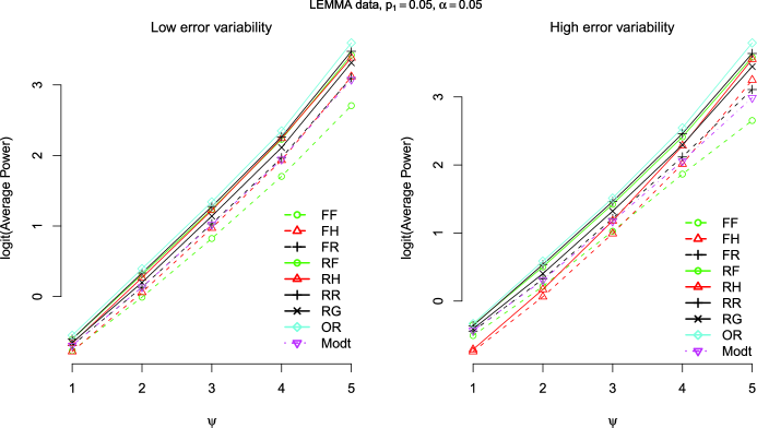
Figure 1: Average power (on the logit scale) for empirical quantile analysis under the RR data generation model, with $n_{1}=n_{2}=6,$ $S=100$ samples, $G=2000$ genes, and $p_{1}=0.05$ probability of non-null status. Left: low error variance variability ($\mathit{CV}=0.58$). Right: high error variance variability ($\mathit{CV}=3.16$).

When the data are generated according to theLEMMA model our simulations show that the tests derived from the RR model achieved the highest power for all $\psi\in\Psi$ (and almost identical to the Optimal Rule’s), as can be seen in Figure 1. When the data are generated according to the LIMMA model, the likelihood ratio tests derived from the RR and RG models have nearly identical performance in terms of power as those of the moderated-$t$ statistics and the LIMMA Optimal Rule for all values of $v_{0}$ (figure not shown).

As expected, our simulations also showed that the average power in the homogeneous error variance models (RH, FH) decreases as the error variance variability increases. In general, the random gene models (RR, RF, RH) demonstrate higher average power than their corresponding fixed gene counterparts. Notice also that the performance of moderated-$t$ and the FR statistics are almost identical.

The second performance assessment method did not require computing empirical quantiles, and was based on local f.d.r. criteria. Efron et al. (2001) and Efron (2005) defined local f.d.r. as

$$\operatorname{f.d.r.}(y_{g})=\Pr(\operatorname{null}|Y=y_{g})$$ (18)

for the posterior probability of a gene $g$ being in the null group. Note that this is precisely $1-p_{1,g}(y_{g}),$ where $p_{1,g}(y_{g})$ is given by (3). Since $p_{1}$ can only be estimated in the random-mean models, we only considered the local f.d.r. statistics associated with RR, RF and RH. For comparison, we also considered the local f.d.r. statistics for RG and the Optimal Rule, and two types of $B$ statistics computed by the limma package to differentiate between those computed with the default value of $p_{1}=0.01$ [referred to as “Limma(0.01)”] and those computed with the estimated value of $p_{1}$ [referred to as “$\operatorname{Limma}(\hat{p}_{1})$”]. We also included local f.d.r. statistics computed from the locfdr (Efron, Turnbull and Narasimhan, 2008) R package (referred to as “Efron” for simplicity).

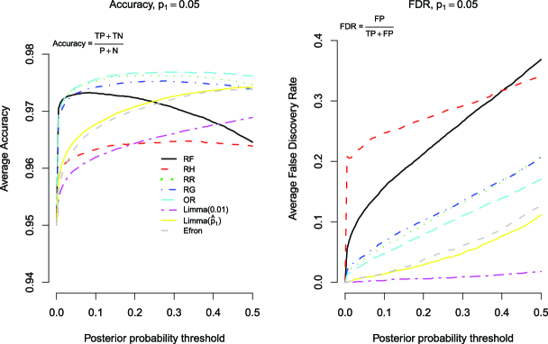
Figure 2: Accuracy (left) and false discovery rate (right) for data generated under the LEMMA model with $n_{1}=n_{2}=6,$ $S=100$ samples, $G=2000$ genes, and $\psi=3$, $p_{1}=0.05$ probability of non-null status, and high error variance variability ($\mathit{CV}=3.16$).

To evaluate the performance of these procedures, we looked at two complementary metrics. The first is the measure of accuracy, defined by the ratio $(\mathit{TP}+\mathit{TN})/(P+N)$ as in Hong (2009), where $P$ and $N$ are the total numbers of non-null and null genes, respectively, and $\mathit{TP}+\mathit{TN}$ is the sum of correct classifications (true positives plus true negatives). The second metric is the false discovery rate, defined by $\mathit{FP}/(\mathit{FP}+\mathit{TP})$, where FP is the total number of false positives. Clearly, our goal is to maximize the accuracy while maintaining a low false discovery rate. To compare different methods, we computed the accuracy and FDR for a range of posterior null probability thresholds (between 0 and 0.5). A gene is declared as non-null if its posterior null probability is below the selected threshold. Note that when the threshold is 0, all genes are declared as null and we obtain accuracy of $1-p_{1}$. As we increase the threshold, the total number of detections increases, and if we let the threshold be 1, all genes are declared as non-null (and the accuracy is $p_{1}$).

Figures 2 and 4 demonstrate that when the data are generated under the LEMMA model, the RR procedure achieves the highest level of accuracy for any posterior probability threshold in the range [0, 0.5], and is practically the same as the Optimal Rule. It has only a slightly higher FDR, compared with the Optimal Rule. Note that RF has high accuracy, but very high FDR, indicating it is too liberal and declares too many genes as non-null.

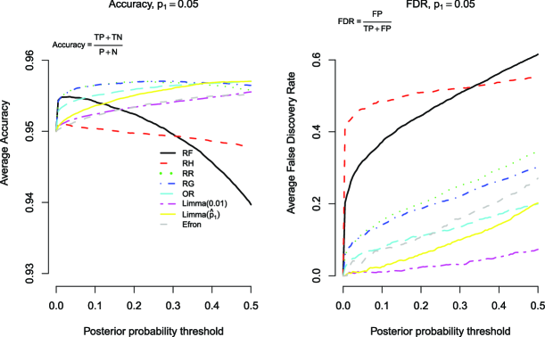
Figure 3: Accuracy (left) and false discovery rate (right) for data generated under the LEMMA model with $n_{1}=n_{2}=6,$ $S=100$ samples, $G=2000$ genes, and $\psi=3$, $p_{1}=0.25$ probability of non-null status, and high error variance variability ($\mathit{CV}=3.16$).

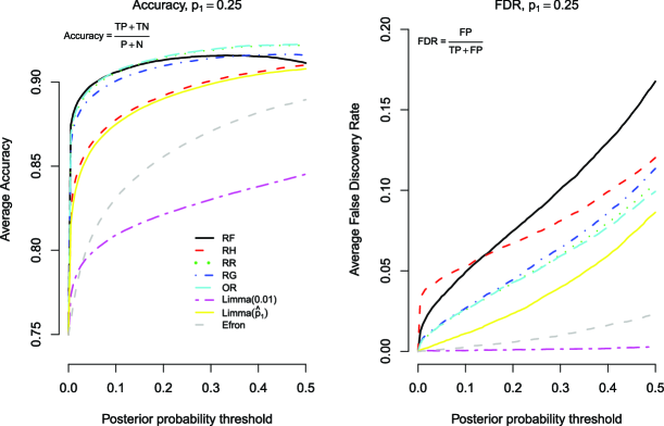
Figure 4: Accuracy (left) and false discovery rate (right) for data generated under the LIMMA model with $n_{1}=n_{2}=6,$ $S=100$ samples, $G=2000$ genes, and $v_{0}=1$, $p_{1}=0.05$ probability of non-null status, and high error variance variability ($\mathit{CV}=3.16$).

We also observe that the RR and RG procedures are quite similar, which is an indication that the choice of the non-null variance model (either $\sigma^{2}_{\psi}$ as in LEMMA, or $v_{0}\sigma^{2}_{\varepsilon,g}$ as in LIMMA) does not have a significant impact on the performance. We also notice that when the limma package is used with the estimated value of $p_{1}$, instead of the default, the accuracy is greatly improved, with a relatively small increase in FDR. Still, the RR procedure (under the LEMMA data generation scheme) is clearly superior to all other methods.

Interestingly, when the data are generated under the LIMMA model, we get similar results—the RR procedure achieves higher accuracy, and only a relatively small increase in false discoveries (see Figures 3 and 5). It is also interesting that the limma procedure does not achieve the performance of its Optimal Rule, and we believe this is due to inaccurate estimation of $p_{1},$ as demonstrated below. Note that lemma uses maximum likelihood estimation for all the model parameters, while limma uses ad-hoc methods to estimate $p_{1}$ and $v_{0}$. In summary, lemma and its RG variant are competitive with limma when LIMMA is the true data generating model, but they are clearly superior when LEMMA is the true data generating model. Furthermore, the additional parameters ($\tau,\psi$) in the LEMMA model do not add to the computational complexity, as the maximum likelihood estimators are obtained via a simple, and fast EM algorithm.

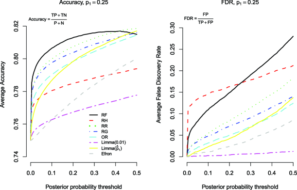
Figure 5: Accuracy (left) and false discovery rate (right) for data generated under the LIMMA model with $n_{1}=n_{2}=6,$ $S=100$ samples, $G=2000$ genes, and $v_{0}=1$, $p_{1}=0.25$ probability of non-null status, and high error variance variability ($\mathit{CV}=3.16$).

To conclude this subsection, we remark that although it is possible to compute posterior probabilities using the limma package (which involves plugging in the estimates for $v_{0}$ and $p_{1}$), in practice, inference via the limma package is often frequentist in nature (using the $p$-values, computed from the $t$-statistics, returned by the eBayes function).

5.3 Estimation Performance

We also analyzed the parameter estimation performance of the lemma software, and we found it to be very accurate when the data are generated under the LEMMA model. However, since this is not unexpected, we chose to present a more interesting result. Recall that both LEMMA and LIMMA require estimation of the non-null prior probability, $p_{1}$. We compared the estimation of this important parameter under those two data generation models using four estimation methods, including lemma, convest (from the limma package) and two estimation procedures available in the locfdr package—denoted by EF-MLE and EF-CME. Smyth (2004) argues that the mixture proportion parameter is difficult to estimate in the model leading to the $B$-statistic, and our simulations verify that the estimates of $p_{1}$ produced by the limma package are significantly biased. (As noted earlier, the limma package uses value of $p_{1}=0.01$, rather than an estimate.) Figure 6 shows that when $p_{1}=0.05$ lemma tends to slightly overestimate the parameter, while the other methods tend to underestimate it. This is in agreement with the observation that lemma achieves higher accuracy, and has a slightly higher FDR. We also point out that both estimation methods available in the locfdr package not only underestimate $p_{1}$, but also give unreasonable (negative) estimates. The lemma estimation procedure is significantly better than the other three for higher values of $p_{1}$, even when the data are generated under the LIMMA model.

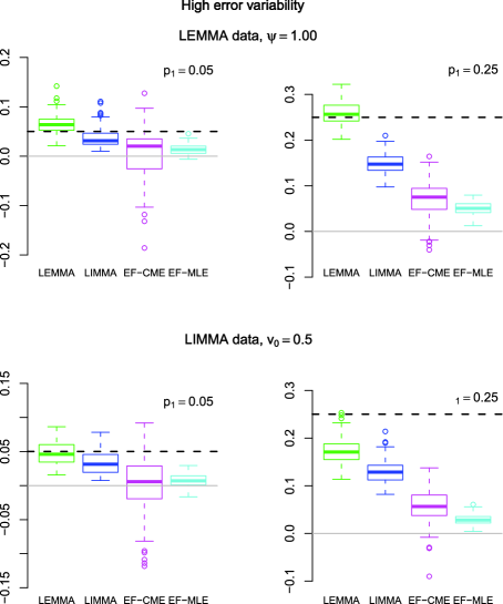
Figure 6: Estimates of $p_{1}$ when the data are generated under the LEMMA model (top) and under LIMMA (bottom), when the true values of $p_{1}$ are 0.05 (left) and 0.25 (right).

6 Examples

Using the lemma software, we fitted the LEMMA model to several microarray data sets. For illustration purposes, we provide our analysis of two publicly available, two-channel gene expression microarray data sets that were previously analyzed: the ApoA1 data (Callow et al., 2000) and the Colon Cancer data (Alon et al., 1999).

6.1 ApoA1 Data

The ApoA1 experiment (Callow et al., 2000) used gene targeting in embryonic stem cells to produce mice lacking apolipoprotein A-1, a gene known to play a critical role in high density lipoprotein (HDL) cholesterol levels. Originally, 5600 expressed sequence tags (EST) were selected. In our analysis, we used the data and normalization method provided with the limma R package (Smyth, 2005), which consists of 5548 ESTs, from 8 control (wild type “black six”) mice and 8 “knockout” (lacking ApoA1) mice. Common reference RNA was obtained by pooling RNA from the control mice, and was used to perform expression profiling for all 16 mice. Note that the current version of the limma user’s guide refers to a larger data set which contains 6384 ESTs. Qualitatively speaking, using the larger data set does not yield different results (in terms of detecting significant genes).

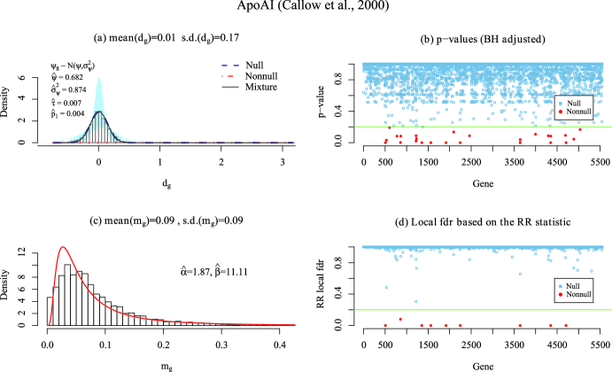
Figure 7: (a) Histogram of the 5548 $d_{g}$ statistics from the ApoA1 data set and the fitted distributions. (b) The Benjamini–Hochberg adjusted $p$-values for all genes. Using an FDR level of 0.2, we detect 25 non-null genes. (c) Histogram of the $m_{g}$ statistics and the fitted distribution. (d) The RR test statistics of all the genes. Using a 0.2 threshold for the posterior probability, we declare 9 genes to be non-null.

The response of interest, $y_{ijg}$, is the $\log_{2}$ fluorescence ratio (with respect to the common reference) where $g$ is one of 5548 genes, $j=1,\ldots,8$ (mouse number), and $i$ is the population index (control and knockout). Using the EM algorithm, we obtained estimates for the parameters in our LEMMA model. Figure 7(a) depicts the histogram of the 5548 $d_{g}$ statistics. The smooth black curve shows the fitted mixture distribution, drawn using the average estimated error variance. The smooth blue and red curves correspond to the average fitted distributions of the null and non-null groups, respectively. Per-gene fitted distributions are plotted in light colors (note that the non-null probability is very small, so only gene-specific distributions of the null group, in light blue, can be observed in this case). The mean-effect parameter estimates we obtained are $\hat{\tau}=0.007$ and $\hat{\psi}=0.682$, $\hat{\sigma}_{\psi}^{2}=0.874$.

Figure 7(c) depicts the histogram of the $m_{g}$ statistics and the fitted distribution. The estimates for the shape and scale parameters of the error variance distribution are 1.87 and 11.11, respectively. The empirical mean and variance of $\{\tilde{\sigma}^{2}_{\varepsilon,g}\}$ are 0.078 and 0.004.

Using the lemma package, we obtained the parameter estimates, and computed the gene-specific posterior probabilities and the $p$-values for the hypotheses that genes are in the null group. Figure 7(b) depicts the Benjamini–Hochberg adjusted $p$-values. The red, solid points represent the genes that were declared non-null, using a (liberal) FDR threshold of 0.2. Using the FDR criteria, we detected 25 non-null genes.

Using the posterior probabilities derived from the LEMMA (RR) model and Efron’s 0.2 threshold for local f.d.r., we detected 9 non-null genes, including the ApoA1 gene and others that are closely related to it. The top eight genes had local f.d.r. values of nearly zero, while the ninth had a much higher value of 0.08. Figure 7(d) depicts the RR local f.d.r. statistics, and the red, solid points represent the genes that were declared non-null using a local f.d.r. threshold of 0.2. The top eight genes (using either the FDR or the local f.d.r. criteria) are also identified (among others) when using the limma and locfdr R packages, and were confirmed to be differentially expressed in the knockout versus the control line by an independent assay.

Interestingly, assuming no other genes are in the non-null group, the true value of $p_{1}$ is 0.00144, and the estimate obtained from lemma is 0.0039, while Efron’s estimates using the MLE and CME methods are $-$0.036 and $-$0.083, respectively. As we mentioned earlier, by default the limma R package does not provide an estimate for $p_{1}$, and uses a value of 0.01. However, using the convest function, limma provides the estimate $p_{1}=0.30$. When one uses the larger ApoA1 data set currently referred to by the limma user’s guide (with 6384 ESTs), the estimate for $p_{1}$ is 0.134.

6.2 Colon Cancer Data

The data analyzed by Alon et al. (1999) consists of 2000 ESTs in 40 tumor and 22 normal colon tissue samples. Of the 40 patients involved in the study, 22 supplied both tumor and normal tissue samples. In their analysis, Alon et al. (1999) used an Affymetrix oligonucleotide array complementary to more than 6500 human genes and expressed sequence tags (ESTs), and a two-way clustering method to identify families of genes and tissues based on expression patterns in the data set. Do, Müller and Tang (2005) used a Bayesian mixture model to analyze the same data set and estimated the probability of differential expression. Using empirical Bayes methods, they obtained a point estimate $\hat{p}_{0}=0.39$ and contrasted it with the posterior marginal probability distribution of $p_{0}$ from the nonparametric Bayesian model, which they fit using MCMC simulations. The empirical Bayes estimate for $p_{0}$ was far out in the right tail of the posterior distribution, which, they argued, might lead to underestimating the posterior probability of being in the non-null group (differentially expressed genes). They propose using posterior expected FDR (Genovese and Wasserman, 2002) thresholds to calibrate between a desired false discovery rate and the number of significant genes. For example, with FDR${}={}$0.2, they find 1938 non-null genes.

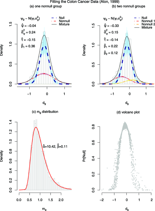
Figure 8: Histograms of the 2000 $d_{g}$ statistics from the Alon et al. (1999) data set and the fitted distributions, assuming (a) a two-group model, or (b) three-group model. (c) Histogram of the $m_{g}$ statistics and the fitted distribution. (d) Volcano plot, showing the posterior null probabilities by $d_{g}$.

Using lemma and assuming the two-group LEMMA model, we obtain $\hat{p}_{1}=0.36$. According to this model, the (non-null) mean effect of the gene-specific term is estimated by $\hat{\psi}=-0.04$ (and the variance by $\hat{\sigma}_{\psi}^{2}=0.24$), and the fitted two-group mixture distribution is shown in Figure 8(a). The near-zero mean of the non-null mixture component suggests that there may be two non-null groups (over- and under-expressed groups of genes). We fitted the three-group variant of the LEMMA model to the data, and obtained $\hat{p}_{1}=0.22,\hat{p}_{2}=0.12,$ and $\hat{\psi}=-0.33,\hat{\sigma}_{\psi}^{2}=0.15$ [see Figure 8(b)]. In Figure 8(a) and (b) the light blue and purple curves represent the (per gene) fitted distributions for the null and non-null groups, respectively. The smooth black curve shows the fitted mixture distribution, drawn using the average estimated error variance.

The three-group model allows for asymmetry in the proportions of over- and under-expressed genes. We see no reason to assume that these proportions should be equal. However, we find in simulations that if they are indeed equal, our procedure estimates them accurately. We have observed that if the true model has two non-null groups, then estimating it assuming two modes results in an estimate of $\psi$ that is biased toward 0 and an inflated $\hat{\sigma}^{2}_{\psi}$ (as seen in this case), and that this could lead to fewer true discoveries.

In this data set, the empirical mean and variance of $m_{g}$ are 1.00 and 0.17, respectively, with estimates $\hat{\alpha}=10.42$ and $\hat{\beta}=0.11$. Figure 8(c) shows the histogram of the $m_{g}$ statistics and the fitted distribution.

The “volcano plot” in Figure 8(d) depicts the posterior null probability of genes based on the three-group LEMMA model versus the $d_{g}$ statistics. Using the null posterior probability threshold of 0.2, we detect 170 non-null genes, while using the FDR method (with a threshold of 0.2) we get 155 genes. Detecting non-null genes in a typical microarray gene expression analysis involves setting a minimum fold-change threshold, in addition to setting the level at which the False Discovery Rate is controlled. For instance, requiring that $|d_{g}|\geq 1$ and controlling the False Discovery Rate at 0.1, we detect 61 non-null genes, all of which were detected by at least one method in Su et al. (2003).

7 Discussion

In the previous sections we demonstrated that our modeling framework can lead to six different test statistics depending on the assumptions imposed on the gene-specific effects. Interestingly, the test statistics associated with these models have been considered independently in the literature in various forms, but to our knowledge, this is the first time they have been categorized as special cases of the same model. The LEMMA (RR) model, in which both the non-null gene-specific effects and gene-specific variances are modeled as random variates, leads to James–Stein-type (shrinkage) estimation of the parameters. Specifically, the statistics derived from the RR model enjoy shrinkage in both the numerator and denominator of a posterior $t$-statistic, resulting in powerful test statistics while maintaining few false positives in our simulation studies. Using a Laplace approximation to make the EM algorithm tractable, our approach yields stable parameter estimates, even for the notoriously difficult parameter $p_{1}$.

Since our approach is model-based, it can be easily generalized to other situations. For example, as stated earlier, the methods described in this paper can be extended to deal with multiple treatments, paired tests (one group) and multiple non-null components. Furthermore, it is straightforward to add fixed-effect covariates to the model. We are currently working on the next release of the lemma package which will include this feature, in addition to within-group analysis, new plotting and exporting functions, and confidence intervals for parameter estimates. Extending the model to handle multivariate responses is also being investigated.

Appendix

In this section we provide details on some of our previous derivations, and elaborate on the case of multiple treatments.

.1 Empirical Bayes Estimates for $\alpha$ and $\beta$

To obtain an estimate of the error variance in the random error case, recall that

$$\quad m_{g}|\sigma_{\varepsilon,g}^{2}\sim\frac{\sigma_{\varepsilon,g}^{2}}{f_{g}}\chi_{f_{g}}^{2}\equiv\operatorname{Gamma}\biggl{(}\frac{f_{g}}{2},\frac{2\sigma_{\varepsilon,g}^{2}}{f_{g}}\biggr{)}.$$ (19)

We maximize the marginal density of $m_{g}$ numerically to obtain maximum likelihood estimates of $\alpha$ and $\beta$. Given the conditional distribution in (19), we find the marginal density of $m_{g}$ by integrating out $\sigma^{2}_{\varepsilon,g}$. Specifically,

$$f(m_{g}) = \int_{0}^{\infty}f(m_{g}|\sigma^{2}_{\varepsilon,g})f(\sigma^{-2}_{\varepsilon,g})\,d\sigma^{-2}_{\varepsilon,g}$$

$$= \int_{0}^{\infty}\biggl{[}\frac{m_{g}^{{f_{g}}/{2}-1}\exp(-{m_{g}f_{g}}/(2\sigma^{2}_{\varepsilon,g}))}{\Gamma({f_{g}}/{2})({2\sigma^{2}_{\varepsilon,g}}/{f_{g}})^{{f_{g}}/{2}}}\biggr{]}$$

$$\hskip 15.0pt{}\cdot\biggl{[}\frac{\exp(-\sigma^{-2}_{\varepsilon,g}\beta^{-1})}{\Gamma(\alpha)\beta^{\alpha}}(\sigma^{-2}_{\varepsilon,g})^{\alpha-1}\biggr{]}\,d\sigma^{-2}_{\varepsilon,g}$$

$$= \frac{m_{g}^{{f_{g}}/{2}-1}({f_{g}}/{2})^{{f_{g}}/{2}}}{\Gamma({f_{g}}/{2})\Gamma(\alpha)\beta^{\alpha}}$$

$${}\cdot\int_{0}^{\infty}(\sigma^{-2}_{\varepsilon,g})^{{f_{g}}/{2}+\alpha-1}$$

$$\hskip 24.0pt{}\cdot\exp\biggl{[}-\sigma^{-2}_{\varepsilon,g}\biggl{(}\frac{m_{g}f_{g}}{2}+\frac{1}{\beta}\biggr{)}\biggr{]}\,d\sigma^{-2}_{\varepsilon,g}$$

$$= \frac{m_{g}^{{f_{g}}/{2}-1}({f_{g}}/{2})^{{f_{g}}/{2}}}{\Gamma({f_{g}}/{2})\Gamma(\alpha)\beta^{\alpha}}$$

$${}\cdot\frac{\Gamma({f_{g}}/{2}+\alpha)}{({m_{g}f_{g}}/{2}+{1}/{\beta})^{{f_{g}}/{2}+\alpha}}.$$

The final equality in (.1) results from noting that the integral in the third equality is proportional to a $\textrm{Gamma}(f_{g}/2+\alpha,[\beta^{-1}+m_{g}f_{g}/2]^{-1})$ density. We maximize $\sum_{g}{\log(f(m_{g}))}$ with respect to $\alpha$ and $\beta$ to obtain the empirical Bayes estimates $\hat{\alpha}$ and $\hat{\beta}$.

The joint distribution of $m_{g}$ and $\sigma_{\varepsilon,g}$ is given by

$$f(m_{g},\sigma_{\varepsilon,g}^{-2}) = m_{g}^{f_{g}/2-1}f_{g}^{f_{g}/2}(\sigma_{\varepsilon,g}^{-2})^{\alpha-1+f_{g}/2}$$

$$\cdot{}\exp\biggl{\{}-\sigma_{\varepsilon,g}^{-2}\biggl{[}\frac{m_{g}}{2}f_{g}+\frac{1}{\beta}\biggr{]}\biggr{\}}$$

$${}\Big{/}{\biggl{(}\Gamma\biggl{(}\frac{f_{g}}{2}\biggr{)}2^{f_{g}/2}\Gamma(\alpha)\beta^{\alpha}\biggr{)}}.$$

So, conditional on $m_{g}$,

$$\sigma_{\varepsilon,g}^{-2}\sim\operatorname{Gamma}\bigl{(}\alpha+f_{g}/2,(m_{g}f_{g}/2+1/\beta)^{-1}\bigr{)}.$$

Hence, the conditional expectation is

$$E(\sigma_{\varepsilon,g}^{2}|m_{g})$$

$$\quad=\frac{f_{g}/2}{f_{g}/2+\alpha-1}m_{g}+\frac{\alpha+1}{f_{g}/2+\alpha-1}\cdot\frac{1}{(\alpha+1)\beta}$$

$$\quad\approx\frac{f_{g}/2}{f_{g}/2+\alpha-1}m_{g}+\frac{\alpha+1}{f_{g}/2+\alpha-1}\bar{m},$$

and the conditional mode is

$$\mathit{Mode}(\sigma_{\varepsilon,g}^{2}|m_{g})$$

$$\quad=\frac{f_{g}/2}{f_{g}/2+\alpha+1}m_{g}+\frac{\alpha+1}{f_{g}/2+\alpha+1}\cdot\frac{1}{(\alpha+1)\beta}$$

$$\quad\approx\frac{f_{g}/2}{f_{g}/2+\alpha+1}m_{g}+\frac{\alpha+1}{f_{g}/2+\alpha+1}\bar{m}.$$

Note that using the approximation of the mode, $\bar{m}\approx[(\alpha+1)\beta]^{-1},$ in both the posterior mean and posterior mode yields a shrinkage-estimator form. Equivalently, we could replace $(\alpha+1)$ with $(\alpha-1)$ in the conditional expectation and the conditional mode, and obtain shrinkage toward the sample mean of $\{m_{g}\}$.

.2 Maximum Likelihood Estimation of $\phi$

Recall that in the RR method we use the Laplace approximation (3.1), hence, the (approximate) complete likelihood is

$$\tilde{L}_{C}(\phi)$$

$$\quad\propto\prod_{g=1}^{G}L(b_{g},d_{g};\tilde{\sigma}_{g}^{2})$$

$$\quad=\prod_{g=1}^{G}\int L(b_{g};p_{1})L(d_{g}|b_{g};\psi_{g},\tilde{\sigma}_{g}^{2})$$

$$\qquad\hskip 27.0pt{}\cdot f(\psi_{g}|b_{g})\,d\psi_{g}$$

(21)

$$\quad=\prod_{g=1}^{G}\biggl{[}p_{1}^{b_{g}}(1-p_{1})^{1-b_{g}}(2\pi\tilde{\sigma}_{g}^{2})^{-{1}/{2}}$$

$$\hskip 17.0pt\qquad{}\cdot(2\pi\sigma_{\psi}^{2})^{-{b_{g}}/{2}}\exp\biggl{\{}-\frac{1-b_{g}}{2\tilde{\sigma}_{g}^{2}}(d_{g}-\tau)^{2}\biggr{\}}$$

$$\hskip 17.0pt\qquad{}\cdot\int\exp\biggl{\{}-\frac{b_{g}}{2\tilde{\sigma}_{g}^{2}}(d_{g}-\tau-\psi_{g})^{2}$$

$$\hskip 17.0pt\qquad{}-\frac{b_{g}}{2\sigma_{\psi}^{2}}(\psi_{g}-\psi)^{2}\biggr{\}}\,d\psi_{g}\biggr{]},$$

with log-likelihood

$$\ell(\phi) \propto \sum_{g=1}^{G}[(1-b_{g})\log(1-p_{1})+b_{g}\log(p_{1})]$$

$${}-\sum_{g=1}^{G}\biggl{[}\frac{b_{g}}{2}\log(2\pi\sigma_{\psi}^{2})+\frac{1}{2}\log(2\pi\tilde{\sigma}_{g}^{2})\biggr{]}$$

$${}-\frac{1}{2}\sum_{g=1}^{G}b_{g}\log\biggl{(}(2\pi)^{-1}\biggl{(}\frac{1}{\tilde{\sigma}_{g}^{2}}+\frac{1}{\sigma_{\psi}^{2}}\biggr{)}\biggr{)}$$

$${}-\sum_{g=1}^{G}(1-b_{g})\frac{(d_{g}-\tau)^{2}}{2\tilde{\sigma}_{g}^{2}}$$

$${}-\sum_{g=1}^{G}\frac{b_{g}}{2}\biggl{[}\frac{1}{\sigma_{\psi}^{2}+\tilde{\sigma}_{g}^{2}}(d_{g}-\tau-\psi)^{2}\biggr{]}.$$

The estimates (11)–(3.1) are obtained by maximizing the log-likelihood with respect to the parameters, $\phi$.

Although the Laplace approximation is not necessary in the RF and RH models, note that the complete likelihoods and log-likelihoods for the these models are identical to equations (.2) and (.2), with $\tilde{\sigma}_{g}^{2}$ replaced by $\hat{\sigma}_{g}^{2}$ and $\hat{\sigma}_{\varepsilon}^{2}$ (as defined in Section 3.2), respectively.

.3 Multiple Treatments

In the general case we assume $t\geq 2$ treatments $i=1,2,\ldots,t$ assigned to $t$ groups of $n_{1,g},n_{2,g},\ldots,n_{t,g}$ subjects indexed by $j_{1}=1,\ldots,n_{1,g},\ldots,j_{t}=1,\ldots,\break n_{t,g}$, and we use the model defined by (1) and (2). Here, we impose a standard (fixed effect) constraint

$$\sum_{i=1}^{t}\psi_{ig}=0.$$

The distributions for the gene-specific effects in the multiple-treatment case are assumed to follow a normal distribution,

$$\bolds{\psi}_{g}\sim\mbox{i.i.d.}~{}N_{t}\bigl{(}\bolds{\psi},\sigma_{\psi}^{2}(\mathbf{I}_{t}-\mathbf{\bar{J}}_{t})\bigr{)},$$

where $\mathbf{I}_{t}-\mathbf{\bar{J}}_{t}$ is the $t\times t$ centering matrix, $\bolds{\psi}$ is a $t$-dimensional vector, and $\sigma_{\psi}^{2}$ is a scalar. The test statistic $m_{g}$ is defined as

$$m_{g}=\sum_{i=1}^{t}\sum_{j=1}^{n_{ig}}(y_{ijg}-\bar{y}_{i\cdot g})^{2}/f_{g},$$

where $f_{g}=n_{1g}+\cdots+n_{tg}-t$, and we use $m_{g}$ as before, to estimate $\alpha$ and $\beta$.

To estimate the rest of the parameters in the LEMMA model, we use the ($t-1$-dimensional vector) test statistics

$$\mathbf{d}_{g}=\mathbf{H\bar{Y}}_{g},$$

where

$$\mathbf{H} = \left[\matrix{1/\sqrt{2}&-1/\sqrt{2}&0\cr 1/\sqrt{6}&1/\sqrt{6}&-2/\sqrt{6}\cr\vdots&\vdots&\vdots&\cr 1/\sqrt{t(t-1)}&1/\sqrt{t(t-1)}&1/\sqrt{t(t-1)}}\right.$$

$$\hskip 80.0pt{}\left.\matrix{\cdots&0\cr\cdots&0\cr&\vdots\cr\cdots&-(t-1)/\sqrt{t(t-1)}}\right],$$

$$\mathbf{\bar{Y}}_{g} = (\bar{Y}_{1\cdot g},\bar{Y}_{2\cdot g},\ldots,\bar{Y}_{t\cdot g})^{\prime}.$$

Derivations similar to the ones we used to obtain the estimates in Section 3 lead to the same estimate for $p_{1}$ and to the following estimates, analogous to (12) and (3.1):

$$\bigl{(}\mathbf{H}{\bolds{\tau}}^{(m+1)}\bigr{)}^{\prime}$$

$$\quad=\Biggl{[}\sum_{g=1}^{G}p^{(m)}_{0,g}\mathbf{d}_{g}^{\prime}\bolds{\Lambda}_{0}^{-1}\Biggr{]}\Biggl{[}\sum_{g=1}^{G}p^{(m)}_{0,g}\bolds{\Lambda}_{0}^{-1}\Biggr{]}^{-1},$$

$$\bigl{(}\mathbf{H\bolds{\psi}}^{(m+1)}\bigr{)}^{\prime}$$

$$\quad=\Biggl{[}\sum_{g=1}^{G}p^{(m)}_{1,g}\bigl{(}\mathbf{d}_{g}-\mathbf{H}\bolds{\tau}^{(m+1)}\bigr{)}^{\prime}(\bolds{\Lambda}_{0}+\bolds{\Lambda}_{A})^{-1}\Biggr{]}$$

$$\qquad{}\cdot\Biggl{[}\sum_{g=1}^{G}p^{(m)}_{1,g}(\bolds{\Lambda}_{0}+\bolds{\Lambda}_{A})^{-1}\Biggr{]}^{-1},$$

where

$$\bolds{\Lambda}_{A} = \sigma_{\psi}^{2(m)}\mathbf{I}_{t-1},$$

$$\bolds{\Lambda}_{0} = \tilde{\sigma}_{\varepsilon,g}^{2}\mathbf{H}[\operatorname{diag}_{i}(1/n_{ig})]\mathbf{H}^{\prime}.$$

The update for $\tilde{\sigma}_{\psi}^{2}$ is the solution to the equation,

$$\sum_{g=1}^{G}p^{(m)}_{1,g}\cdot\operatorname{tr}\bigl{(}(\bolds{\Lambda}_{0}+\bolds{\Lambda}_{A})^{-1}\bigr{)}$$

$$\quad=\sum_{g=1}^{G}p^{(m)}_{1,g}\bigl{(}\mathbf{d}_{g}-\mathbf{H}\bolds{\xi}^{(m+1)}\bigr{)}^{\prime}(\bolds{\Lambda}_{0}+\bolds{\Lambda}_{A})^{-2}$$

$$\qquad{}\cdot\bigl{(}\mathbf{d}_{g}-\mathbf{H}\bolds{\xi}^{(m+1)}\bigr{)},$$

where $\bolds{\xi}^{(m+1)}=\bolds{\tau}^{(m+1)}+\bolds{\psi}^{(m+1)}$.

The likelihood ratio test statistic has a similar form as (4),

$$\frac{L_{0,g}}{L_{1,g}} = |\mathbf{I}-\bolds{\Lambda}_{g}|^{-1/2}\exp\biggl{\{}-\frac{1}{2}\bolds{\Gamma}^{\prime}(\bolds{\Lambda}_{0}^{-1}\bolds{\Lambda}_{g}^{-1})\bolds{\Gamma}\biggr{\}}$$

$${}\cdot\exp\biggl{\{}-\frac{1}{2}\tilde{\sigma}_{\psi}^{-2}(\mathbf{H}\hat{\bolds{\psi}})^{\prime}(\mathbf{H}\hat{\bolds{\psi}})\biggr{\}},$$

where

$$\bolds{\Gamma} = [\bolds{\Lambda}_{g}(\mathbf{d}_{g}-\mathbf{H\hat{\bolds{\tau}}})+(\mathbf{I}-\bolds{\Lambda}_{g})(\mathbf{H}\hat{\bolds{\psi}})],$$

$$\bolds{\Lambda}_{g} = (\bolds{\Lambda}_{A}+\bolds{\Lambda}_{0})^{-1}\bolds{\Lambda}_{A},$$

$$\mathbf{I}-\bolds{\Lambda}_{g} = (\bolds{\Lambda}_{A}+\bolds{\Lambda}_{0})^{-1}\bolds{\Lambda}_{0}.$$

References

- Allison et al. (2006) Allison, D. B., Cui, X., Page, G. P. and Sabripour, M. (2006). Microarray data analysis: From disarray to consolidation and consensus. Nat. Genet. 7 55–65.
- Alon et al. (1999) Alon, U., Barkai, N., Notterman, D. A., Gish, K., Ybarra, S., Mack, D. and Levine, A. J. (1999). Broad patterns of gene expression revealed by clustering analysis of tumor and normal colon tissues probed by oligonucleotide arrays. Proc. Natl. Acad. Sci. USA 96 6745–6750.
- Baldi and Long (2001) Baldi, P. and Long, A. D. (2001). A Bayesian framework for the analysis of microarray expression data: Regularized -test and statistical inferences of gene changes. Bioinformatics 17 509–519.
- Bar and Schifano (2009) Bar, H. and Schifano, E. (2009). lemma: Laplace approximated EM Microarray Analysis R package, Version 1.2-1.
- Benjamini and Hochberg (1995) Benjamini, Y. and Hochberg, Y. (1995). Controlling the false discovery rate—a practical and powerful approach to multiple testing. J. Roy. Statist. Soc. Ser. B 57 499–517. \MR1325392
- Butler (2007) Butler, R. W. (2007). Saddlepoint Approximations with Applications. Cambridge Univ. Press, Cambridge. \MR2357347
- Callow et al. (2000) Callow, M. J., Dudoit, S., Gong, E. L., Speed, T. P. and Rubin, E. M. (2000). Microarray expression profiling identifies genes with altered expression in HDL-deficient mice. Genome Res. 10 2022–2059.
- Cui and Churchill (2003) Cui, X. and Churchill, G. A. (2003). Statistical tests for differential expression in cDNA microarray experiments. Genome Biol. 4 210.
- Cui et al. (2005) Cui, X., Hwang, J. T. G., Qui, J., Blades, N. J. and Churchill, G. A. (2005). Improved statistical tests for differential gene expression by shrinking variance components. Biostatistics 6 59–75.
- de Bruijn (1981) de Bruijn, N. G. (1981). Asymptotic Methods in Analysis. Dover, New York. \MR0671583
- Do, Müller and Tang (2005) Do, K.-A., Müller, P. and Tang, F. (2005). A Bayesian mixture model for differential gene expression. J. Roy. Statist. Soc. Ser. C 54 627–644. \MR2137258
- Efron (2005) Efron, B. (2005). Local false discovery rates. Available at http://www-stat.stanford.edu/~ckirby/brad/papers/2005LocalFDR.pdf
- Efron (2008) Efron, B. (2008). Microarrays, empirical Bayes and the two groups model. Statist. Sci. 23 1–22. \MR2431866
- Efron et al. (2001) Efron, B., Tibshirani, R., Storey, J. and Tusher, V. (2001). Empirical Bayes analysis of microarray experiment. J. Amer. Statist. Assoc. 96 1151–1160. \MR1946571
- Efron, Turnbull and Narasimhan (2008) Efron, B., Turnbull, B. B. and Narasimhan, B. (2008). locfdr: Computes local false discovery rates R package, Version 1.1-6. \MR2431866
- Figueroa et al. (2008) Figueroa, M. E., Reimers, M., Thompson, R. F., Ye, K., Li, Y., Selzer, R. R., Fridriksson, J., Paietta, E., Wiernik, P., Green, R. D., Greally, J. M. and Melnick, A. (2008). An integrative genomic and epigenomic approach for the study of transcriptional regulation. PLoS ONE 3 e1882.
- Genovese and Wasserman (2002) Genovese, C. and Wasserman, L. (2002). Operating characteristics and extensions of the false discovery rate procedure. J. Roy. Statist. Soc. Ser. B 64 499–517. \MR1924303
- Hong (2009) Hong, C. S. (2009). Optimal threshold from ROC and CAP curves. Comm. Statist. Simulation Comput. 38 2060–2072.
- Hwang and Liu (2010) Hwang, J. T. G. and Liu, P. (2010). Optimal tests shrinking both means and variances applicable to microarray data. Stat. Appl. Genet. Mol. Biol. 9 article 36.
- Kendziorski et al. (2003) Kendziorski, C. M., Newton, M. A., Lan, H. and Gould, M. N. (2003). On parametric empirical Bayes methods for comparing multiple groups using replicated gene expression profiles. Stat. Med. 22 3899–3914.
- Kerr, Martin and Churchill (2000) Kerr, M., Martin, M. and Churchill, G. (2000). Analysis of variance in microarray data. J. Comput. Biol. 7 819–837.
- Liu (2006) Liu, P. (2006). Sample size calculation and empirical Bayes tests for microarray data, Ph.D. thesis, Cornell Univ.