Graphical Models for Inference Under Outcome-Dependent Sampling

Abstract

We consider situations where data have been collected such that the sampling depends on the outcome of interest and possibly further covariates, as for instance in case-control studies. Graphical models represent assumptions about the conditional independencies among the variables. By including a node for the sampling indicator, assumptions about sampling processes can be made explicit. We demonstrate how to read off such graphs whether consistent estimation of the association between exposure and outcome is possible. Moreover, we give sufficient graphical conditions for testing and estimating the causal effect of exposure on outcome. The practical use is illustrated with a number of examples.

eadsep;

, and

1 Introduction

Nonrandom sampling poses a challenge for the statistical analysis especially of observational data. We focus here on the problem of outcome-dependent sampling, where the inclusion of a unit into the sample depends, possibly in some indirect way, on the outcome of interest, and possibly on further variables. The prime examples are case-control studies, which have been surrounded by a long controversy, but are now one of the most popular designs in observational epidemiology (Breslow, 1996). Any observational study based on volunteers is also potentially sampled depending on the outcome, as the willingness to participate can never be safely assumed to be independent of the outcome of interest, for example, income. In other situations the outcome-dependent sampling may not be obvious, such as retrospective time-to-event studies (Weinberg, Baird and Rowland, 1993).

A superficial statistical analysis will typically be biased under nonrandom sampling. It is therefore important to investigate and understand the assumptions and limitations underlying valid inference in such situations. Most approaches make very specific parametric modeling assumptions, including assumptions about the selection mechanism, sometimes accompanied by a sensitivity analysis (see, e.g., Copas and Li, 1997, or McCullagh, 2008). As an alternative, in this article we investigate the potential of graphical models to address the problem of outcome-dependent sampling and restrict any assumptions to be nonparametric and only in terms of conditional independencies. A graphical model represents variables as nodes and uses edges between nodes so that separations reflect conditional independencies in the underlying model (see, e.g., Whittaker, 1990, or Lauritzen, 1996).

A key element of our proposed approach is to include a separate node as a binary selection indicator in the graph so as to represent structural assumptions about how the sampling mechanism is related to exposure, outcome, covariates and possibly hidden variables. A similar idea appears in the works of Cooper (1995), Cox and Wermuth (1996), Geneletti, Richardson and Best (2009) and Lauritzen andRichardson (2008). Our main results in this article address the (graphical) characterization of situations where the typical null hypothesis of no association or no causal effect can be tested, and, when all variables are categorical, where (causal) odds ratios can be consistently estimated. These graphical rules do not require particular parametric constraints and essentially capture when the model is collapsible over the selection indicator. While our results on testing are general, estimation is restricted to odds ratios as these (or functions thereof) are the only measures of association that do not depend on the marginal distributions (Edwards, 1963; Altham, 1970) and for which results can be obtained without specific parametric assumptions.

The outline of the article is as follows. In Section 2 we review basic concepts of graphical models, and highlight how a binary sampling node can be included so as to make assumptions about the sampling process explicit (Section 2.4). The corresponding graphs can be constructed in different ways, for instance in a prospective or retrospective manner representing different types of assumptions. Section 3 revisits the notion of collapsibility, which is fundamental for being able to ‘ignore’ outcome-dependent sampling. Sections 3.3 and 3.4 provide the central results that allow us to estimate an odds ratio (Corollary 4) or test for an association (Theorem 6) under outcome-dependent sampling. Section 3.5 illustrates this with a data example. We then move on to causal inference in Section 4, where we define a causal effect as the effect of an intervention. We formalize this using intervention indicators, and adapt the graphical representation by adding a corresponding decision node yielding so-called influence diagrams (Dawid, 2002). In analogy to the associational case, Theorem 7 establishes (graphically verifiable) conditions under which a prospective causal effect can be tested or estimated from retrospective, that is, outcome-dependent, data. In Section 5 we present new results that apply to less obvious cases of outcome-dependent sampling (Theorems 8 and 9).

2 Graphical models

We start with a brief overview of graphical models. Our notation follows closely that of Lauritzen (1996). A graph $G=(V,E)$ with nodes or vertices $V$ and edges $E$ is combined with a statistical model, that is, a distribution $P$ on a set of variables that are identified with the nodes of the graph. The distribution $P$ has to be such that the absence of an edge in the graph represents a certain conditional independence between the corresponding pair of variables. Conditional independence of $A$ and $B$ given $C$ is denoted by $A\perp\!\!\!\perp B|C$ (Dawid, 1979).

The type of graph dictates the specific conditional independence induced by the absence of an edge. A basic distinction is between undirected graphs, directed acyclic graphs (DAGs) and chain graphs. We review the former two but do not go into detail for chain graphs.

2.1 Undirected Graphs

In an undirected graph $G$ all edges are undirected, represented by $a$–$b$. All nodes in $V\backslash\{a\}$ that have an edge with $a\in V$ form the boundary $\operatorname{bd}(a)$ of $a$. We say that two sets of nodes $A$ and $B$ are separated by a third set $C$ if any path along the edges of the graph between $A$ and $B$ includes vertices in $C$. In particular, each set $A$ is separated by its boundary from all other nodes $V\backslash(\mathrm{bd}(A)\cup A)$. The induced conditional independencies are as follows. For any disjoint subsets $A,B,C\subset V$, the variables in $A$ have to be conditionally independent of those in $B$ given $C$ whenever $C$ separates $A$ and $B$ in the graph—we then call $P$ $G$-Markovian. As examples consider the undirected graphs in Figure 1. In the left graph, $X\perp\!\!\!\perp C|(B,Y)$ as well as $Y\perp\!\!\!\perp B|(C,X)$. In the right graph of Figure 1, for instance, $B_{1}\perp\!\!\!\perp B_{2}|(C,Y)$ or $B_{1}\perp\!\!\!\perp B_{2}|(C,X)$ showing that separating sets are not necessarily unique.

We say that a subset $C\subset V$ of the nodes of a graph is complete if each pair of nodes in $C$ is joined by an edge. We further call such a complete $C$ a clique if adding any further node would destroy its completeness; that is, a clique is a maximal complete set of nodes. In Figure 1 the graph on the right has cliques $\{B_{1},C\},\{B_{1},X\},\{X,Y\}$ and $\{B_{2},C,Y\}$.

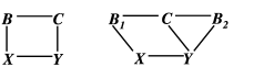
Figure 1: Examples of undirected graphs.

Let $\mathcal{C}$ be the set of all cliques in $G$. The above conditional independence restrictions that are induced by an undirected graph go hand in hand with a factorization of the joint distribution in terms of these cliques. Assume $p$ is the p.d.f. (or p.m.f. if discrete) of the random vector $X_{V}=(X_{1},\ldots,X_{K})$ taking values $x_{V}=(x_{1},\ldots,x_{K})$; then $p$ is said to factorize according to an undirected graph $G$ if it can be written as

$$p(x_{V})=\prod_{C\in\mathcal{C}}\phi_{C}(x_{C}),$$ (1)

where $\phi_{C}(\cdot)$ are functions that depend on $x_{V}$ only through its components in $C$.

In later sections we will also make use of the notion of an induced subgraph $G_{A}$, $A\subset V$, obtained by removing all nodes in $V\backslash A$ and edges involving at least one node in $V\backslash A$.

2.2 Directed Acyclic Graphs

Directed acyclic graphs (DAGs) represent different sets of conditional independencies than undirected graphs. They often seem more natural if one thinks of a data generating process, that is, a way in which the data could be simulated, but DAGs can also be used to represent conditional independencies other than for a generating process. Moreover, one could also use chain graphs (Frydenberg, 1990; Wermuth and Lauritzen, 1990) which represent again different sets of conditional independencies; undirected graphs as well as DAGs are special cases of chain graphs.

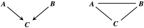
Figure 2: DAG (left) representing $A\perp\!\!\!\perp B$ and moral graph (right) showing $A\perp\!\!\!\perp\diagup\ B|C$.

In DAGs all edges are directed, for example, $a\rightarrow b$, without forming any directed cycles. For $a\rightarrow b$ we say that $a$ is a parent of $b$ and $b$ is a child of $a$. This can be generalized to sets, for example, pa($A$), $A\subset V$, denotes all the variables in $V\backslash A$ that are parents of some variable in $A$, and similarly for the children ch$(A)$. Analogously we speak of descendants de$(A)$ of $A$, meaning all those nodes in $V\backslash A$ that can be reached from some vertex in $A$ following the direction of the edges, while nondescendants nd$(A)$ are all other nodes (excluding $A$ itself). Further, the ancestors an$(A)$ are defined as those nodes in $V\backslash A$ from which we can reach some vertex in $A$ following the direction of the edges.

Similarly to (1), a DAG also induces a factorization of the joint density as follows:

$$p(x_{1},\ldots,x_{K})=\prod_{k=1}^{K}p\bigl{(}x_{i}|x_{\mathrm{pa}(i)}\bigr{)},$$ (2)

where $p(x_{i}|x_{\mathrm{pa}(i)})$ denotes the conditional density of $X_{i}$ given all its parent variables $X_{\mathrm{pa}(i)}$. A simple example is given in Figure 2 (left): here the joint distribution factorizes as $p(a,b,c)=p(a)p(b)p(c|a,b)$.

The factorization (2) is equivalent to the following, graphically characterized conditional independencies:

$$X_{i}\perp\!\!\!\perp X_{\mathrm{nd}(i)\backslash\mathrm{pa}(i)}|X_{\mathrm{pa}(i)}\quad\forall i\in V.$$ (3)

For instance, in Figure 2 (left), $A$ is a nondescendant of $B$ that has no parents, hence $A\perp\!\!\!\perp B$ is implied by this DAG; there is no other (conditional) independence in this particular DAG.

Even though the partial ordering imposed by the direction of the edges on the variables $X_{1},\ldots,X_{K}$ is often postulated to follow some causal or time order, this does not automatically follow from the represented conditional independencies (cf. Section 2.4). For instance $p(a,b,c)=p(a)p(c|a)p(b|c)$ implies the same conditional independencies as $p(a,b,c)=p(b)p(c|b)p(a|c)$, represented in the two graphs $A\rightarrow C\rightarrow B$ and $A\leftarrow C\leftarrow B$, respectively. In both cases $A\perp\!\!\!\perp B|C$. These two graphs (or factorizations) are called Markov equivalent, meaning that exactly the same conditional independencies can be read off. This implies that even if we believe there is an underlying unknown causal or other kind of ordering, then conditional independencies estimated from observational data on $A,B,C$ cannot help to distinguish between these graphs nor tell us the causal order. However, depending on the way in which the variables are observed, how a study is conducted or other considerations, it might seem more natural to specify $p(c|a)$ and $p(b|c)$ than $p(c|b)$ and $p(a|c)$ (we will come back to this below). Note that the DAG of Figure 2 is not equivalent to the former two as it induces a different independence, $A\perp\!\!\!\perp B$.

2.3 Selection Effect and Moralization

All conditional independencies that can be deduced from (3) are given by graph separation for DAGs. One can either use the d-separation criterion (Verma and Pearl, 1988) or the moralization criterion (Lauritzen et al., 1990). The latter is described in detail next.

The moralization criterion is used to determine the conditional independencies of a DAG $G$ in a collection of undirected graphs using ordinary graph separation. These are the moral graphs on subgraphs of $G$. Let $A\subset V$ and let $\operatorname{An}(A)=$ an$(A)\cup A$; then the corresponding moral graph $G_{\mathrm{An}(A)}^{m}$ is given by adding undirected edges between nodes of An$(A)$ that have a common child in An$(A)$ and then turning all remaining directed edges into undirected ones. Any conditional independence that is induced by factorization (2) can be read off $G_{\mathrm{An}(A)}^{m}$ for some $A\subset V$. More specifically, if we want to establish whether $A\perp\!\!\!\perp B|C$, then we check for graph separation in the undirected graph $G_{\mathrm{An}(A\cup B\cup C)}^{m}$. In Figure 2, if we want to investigate whether $A\perp\!\!\!\perp B$, we draw the moral graph $G_{\mathrm{An}(A\cup B)}^{m}$ which consists of the two unconnected nodes $A$ and $B$, with node $C$ removed as it is not in An$(A\cup B)$, confirming that $A\perp\!\!\!\perp B$ as shown earlier. However, if we want to check whether $A\perp\!\!\!\perp B|C$, then we draw the moral graph $G_{\mathrm{An}(A\cup B\cup C)}^{m}$ shown on the right in Figure 2 and see that this independence is not implied by the graphical model.

The “moral edges” represent what is known in epidemiology as selection or stratification (Greenland, 2003; Hernan, Hernández-Díaz and Robins, 2004): if $A$ and $B$ are marginally independent but $C$ depends on both of them, as represented by the DAG in Figure 2, then conditioning on $C$ typically induces a dependence between $A$ and $B$. This can easily be seen as the factorization $p(a,b,c)=p(a)p(b)p(c|a,b)$ does not imply a factorization of $p(a,b|c)=p(a|c)p(b|c)$. As an example assume that $A$ is (binary) exposure to a risk factor and $B$ is some disease indicator that is entirely unrelated to $A$. Further assume that the data are obtained from a database $C$, with $C=1$ if an individual is found in that database and $C=0$ otherwise. If, for some reason, individuals who are exposed are more likely to be in the database as well as individuals who are ill, then we typically find an association between $A$ and $B$ in the sample from that database because we condition on $C=1$. This may, for example, happen when it is a database for a different disease for which $A$ is a risk factor and which is associated with $B$ (cf. Berkson, 1946). In this example, the marginal association of $A$ and $B$ is the target of inference, but cannot be obtained from the available data, so that this phenomenon is often called selection (or stratification) bias. Note that in econometrics the term selection bias is also used to denote systematic (as opposed to randomized) selection into treatment or exposure (Heckman, 1979), which in epidemiology would rather be called confounding.

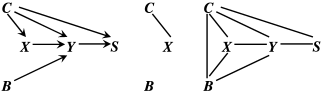
Figure 3: DAG (left) with moral graphs on ${\operatorname{An}(B\cup X)}$ (middle) and on ${\operatorname{An}(B\cup X\cup S)}$ (right).

The selection effect is equally relevant when conditioning is not on a common child of nodes $A$ and $B$ but on any descendant of such a common child as this indirectly provides information on all ancestors; for example, in Figure 3 (left), $X\perp\!\!\!\perp B$ but $X\perp\!\!\!\perp\diagup\ B|S$ because $S$ carries some information on $Y$ and $Y$ is a common child of $B$ and $X$. Figure 3 shows the corresponding moral graphs $G_{\mathrm{An}(B\cup X)}^{m}$ (middle) and $G_{\mathrm{An}(B\cup X\cup S)}^{m}$ (right) for checking these two conditional independence statements.

2.4 Graphical Representation of Sampling Mechanisms

We now turn to the question of how to represent with graphical models that the units in the dataset have possibly been sampled depending on some of the variables relevant to the analysis. The nodes include $X$, the exposure or treatment, and $Y$, the response. Additional nodes are used to represent further relevant variables, for example, in particular a binary variable $S$ indicating whether the unit is sampled, $S=1$, or not, $S=0$. This use of a sampling indicator has also been proposed by Cooper (1995), Cox and Wermuth (1996), Geneletti, Richardson and Best (2009) and Lauritzen and Richardson (2008). Also, we may include a set of covariates $C$.

The graph is normally constructed based on a combination of subject matter background knowledge, especially concerning the sampling mechanism, and testable implications. Some examples for different sampling mechanisms are depicted in Figure 4. Note that all the graphs in Figure 4 could as well be undirected (replacing every directed edge by an undirected one) and still represent the same conditional independencies, that is, $S\perp\!\!\!\perp(X,Y,C)$ in (a), $S\perp\!\!\!\perp(X,Y)|C$ in (b), $S\perp\!\!\!\perp(X,C)|Y$ in (c) and $S\perp\!\!\!\perp X|(Y,C)$ in (d).

(a)	(b)	(c)	(d)

Figure 4: DAGs for different sampling processes: (a) independent sampling, (b) stratified (on covariates $C$) sampling, (c) case-control sampling, (d) case-control matched by $C$.

For a given set of variables we speak of outcome-dependent sampling if $Y$ and $S$ are dependent whatever subset of the remaining variables we condition on, such as in (c) and (d) of Figure 4. The problem created by outcome-dependent sampling is that, first, $p(y)$ cannot be identified as the observations are only informative for $p(y|S=1)$, and second, that conditioning on $S=1$ might create associations that are not present in the target population due to the selection effect as explained in Section 2.3 (Hernan, Hernández-Díaz and Robins, 2004). For a DAG to represent the selection effect, it has to be constructed in a prospective way, as in Figure 4 and as illustrated in the following example.

In Figure 3, assume that $B$ and $C$ are baseline covariates like $B={}$sex and $C={}$age, while $X$ is exposure to a risk factor (e.g., loud music) that possibly changes with age but not with sex and $Y$ is a disease (e.g., hearing loss) that is affected by all previous variables. Assume further that we select individuals into our study, $S=1$, based on age and disease status (as would be the case in a case-control study matched by age); hence $S$ depends on $C$ and $Y$. A DAG on the partially ordered variables $(\{B,C\},X,Y,S)$ would reflect the time order in which the variables are assumed to be realized, and would enable us to express, for instance, the assumption that $B\perp\!\!\!\perp X$ as shown in Figure 3. It also allows us to represent that the sampling induces dependencies that are not present marginally, that is, the selection effect. The DAG in Figure 3, for instance, implies that the joint density of all variables factorizes as

$$p(s,y,b,c,x)$$

$$\quad=p(s|y,c)p(y|x,b,c)p(x|c)p(b)p(c).$$

Data from a case-control study, however, only admits inference on the conditional distribution given $S=1$ which is given by

$$p(y,b,c,x|S=1)$$

(4)

$$\quad=\frac{p(S=1|y,c)p(y|x,b,c)p(x|c)p(b)}{\sum_{y,c}p(S=1|y,c)p(c)p(y|c)}.$$

Marginalizing this over $Y$ shows that there are no necessary independencies among $\{X,B,C\}$ conditional on $S=1$ confirming that $\{X,B,C\}$ must be complete in $G_{\mathrm{An}\{X,B,C,S\}}^{m}$ as in the right graph of Figure 3.

As an alternative to the prospective view, one could decide to represent the sampling process, that is, the order imposed by the sampling which will be retrospective under outcome-dependent sampling; in a case-control study, for instance, the response $Y$ is sampled first and hence the remaining variables are conditional on the response.

Continuing the above example, choosing the sampled units ($S=1$) based on age and disease status partially reverses the order to be $(S,\{C,Y\},\{B,X\})$. Conditional independence test on the retrospective data might reveal that $X\perp\!\!\!\perp B|(C,Y)$ which can be represented as in the DAG in Figure 5 (cf. moral graph on the right). While this conditional independence can be tested from case-control data, the marginal independence $B\perp\!\!\!\perp X$ postulated in Figure 3 cannot be tested from case-control data due to the properties of (2.4). (The latter could, however, be checked approximately, when the disease is rare, using only the controls.)

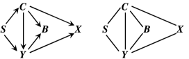
Figure 5: Representing the sampling order: DAG (left) with moral graph on $\operatorname{An}(B\cup X\cup C\cup Y)$ (right).

A DAG reflecting the sampling order allows us to encode conditional independencies given that a unit is sampled. While this makes it typically more difficult to include any subject-specific background knowledge about the data generating process in the formulation of the graph, it might result in a model that fits the data better and still provides consistent, and simpler, estimates of the parameter we are interested in. For a causal analysis, however, where we want to be able to express prior causal assumptions, it is crucial that the graph reflects the prospective view (see Section 4.1). In particular we want to encode which variables are potentially affected by an external change in the exposure status $X$ by representing these as descendants of $X$ in the graph. The causal interpretation of DAGs will be discussed in more detail in Section 4; until then we focus on graphs representing conditional independencies.

3 Collapsibility

Roughly speaking, collapsibility means that inference can be carried out on a subset of the variables, that is, after marginalizing over others (an exact definition for odds ratios is given below). Typically collapsibility is exploited to reduce dimensionality and computational effort, as it enables us to pool subgroups. In our context collapsibility is relevant for the opposite reason: all that we have is a subgroup, namely the sampled population; but we want the associations found in this subgroup to be valid for the whole target population.

In this section we focus on the odds ratio as a measure of association. This is motivated by the fact that the odds ratio does not depend on the marginal distribution of $Y$, which is potentially affected by the sampling process, this also being the main reason why odds ratios are typically used for case-control data. We revisit general results on collapsibility of odds ratios, including their graphical versions, and then modify these to deal with the particular problem of outcome-dependent sampling. Note that the results concerning odds ratios given next are closely linked to graphical log-linear models (Darroch et al., 1980; Lauritzen, 1996, Chapter 4).

3.1 Conditional Odds Ratios

Define the conditional odds ratio $\mathit{OR}_{YX}(C=c)$ (in short we also write $\mathit{OR}_{YX}(C)$) for binary $Y$ and binary $X$ given $C=c$ as

$$\frac{p(Y=1|X=1,C=c)p(Y=0|X=0,C=c)}{p(Y=0|X=1,C=c)p(Y=1|X=0,C=c)}.$$

It is straightforward to generalize this for the case where $Y$ and $X$ have more than two categories. We might then consider a collection of (conditional) odds ratios comparing the probabilities for $Y=y$ versus a reference category $Y=0$ for values of $X$, say $X=x$ versus $X=0$. This collection of odds ratios fully characterizes the (conditional) dependence between $X$ and $Y$ and is, vice versa, fully determined by the corresponding interaction terms of a log-linear model. The results given below can therefore easily be extended to the case of more than two categories.

3.2 General Results

It is well known that the conditional odds ratio $\mathit{OR}_{YX}(C)$ is not necessarily the same as when we collapse over $C$, that is, as the marginal $\mathit{OR}_{YX}$, even if $\mathit{OR}_{YX}(C=c)=\mathit{OR}_{YX}(C=c^{\prime})$ for all $c\not=c^{\prime}$. Though this property is at the heart of most definitions of collapsibility, there are some subtleties giving rise to various definitions of, and different conditions that are sufficient and sometimes necessary for, collapsibility (Bishop, Fienberg and Holland, 1975; Whittemore, 1978; Shapiro, 1982; Davis, 1986; Ducharme and Lepage, 1986; Wermuth, 1987; Geng, 1992; Guo, Geng and Fung, 2001). Here we define collapsibility as follows.

Definition 1.

Consider two binary variables $X$ and $Y$ and disjoint sets of further variables $B$ and $C$. We say that the odds ratio $\mathit{OR}_{YX}(B,C)$ given $B$ and $C$ is collapsible over $B$ if $\mathit{OR}_{YX}(B=b,C=c)=\mathit{OR}_{YX}(B=b^{\prime},C=c)=$ $\mathit{OR}_{YX}(C=c)$, for all $b\not=b^{\prime}$.

Note that in the above definition as well as in all the following results, the covariates $C$ can be of arbitrary measurement level, while $X$, $Y$ and the covariates we consider to collapse over, $B$, are categorical. Collapsibility can then be ensured as follows.

Theorem 2.

Sufficient conditions for the conditional odds ratio $\mathit{OR}_{YX}(B,C)$ to be collapsible over $B$ are: [(ii)]

$Y\perp\!\!\!\perp B|(C,X)$ or

$X\perp\!\!\!\perp B|(C,Y)$.

This follows from the work of Whittemore (1978).

(a) The conditions in Theorem 2 are necessary if $B$ is a single binary variable (Whittemore, 1978).

(b) The conditions in Theorem 2 also ensure, and are necessary for, strong collapsibility which posits that the equality holds for any newly defined $B^{\prime}$ obtained by merging categories of $B$ (Ducharme and Lepage, 1986; Davis, 1986).

The conditions in Theorem 2 are not necessary; the following corollary gives a more general result.

Corollary 3.

Assume that $B$ can be partitioned into $(B_{1},\ldots,B_{K})$, and let $\bar{B}^{k+1}=(B_{k+1},\ldots,B_{K})$. If $B_{k}$ satisfies for each $k=1,\ldots,K$, either: [(ii)]

$Y\perp\!\!\!\perp B_{k}|(C,X,\bar{B}^{k+1})$ or

$X\perp\!\!\!\perp B_{k}|(C,Y,\bar{B}^{k+1})$, then $\mathit{OR}_{YX}(B,C)$ is collapsible over $B$.

With Theorem 2, $\mathit{OR}_{YX}(B_{k},\ldots,B_{K},C)$ is collapsible over $B_{k}$, $k=1,\ldots,K$. Hence we can consecutively collapse over $B_{1},\ldots,B_{K}$.

The conditions of Theorem 2, generalized in Corollary 3, can be checked graphically as they correspond to simple separations in graphical models, regardless whether an undirected graph, a DAG or a chain graph is used to model the data. We consider the case of undirected graphs next; these could also be the moral graphs derived from DAGs or chain graphs.

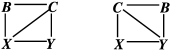
Figure 6: Left graph satisfies (i), right graph satisfies (ii) of Corollary 3.

When $B$ is not partitioned, the graphical equivalents of the two conditions in the above corollary are given in Figure 6, where each of the graphs could have fewer edges but not more. An example where $B$ consists of $B=\{B_{1},B_{2}\}$ and is collapsible is given in Figure 1 (right); $B_{1}$ satisfies (i) and $B_{2}$ satisfies (ii) of Corollary 3. The conditions of Theorem 2 can easily be checked on DAGs as well. For instance, in Figure 7, the graph in (a) satisfies (i) and (b) satisfies (ii) of the theorem (their moral graphs are exactly those in Fig. 6). In contrast, (c) cannot be collapsed over $B$ as the moral graph in (d) shows that neither $B\perp\!\!\!\perp Y|(X,C)$ nor $B\perp\!\!\!\perp X|(Y,C)$ holds in general. Note that the marginal independence $X\perp\!\!\!\perp B$ in this DAG does not help with respect to collapsing the odds ratio over $B$.

(a)	(b)	(c)	(d)

Figure 7: Graphs (a) and (b) satisfy Theorem 2, while graph (c) violates the conditions [moral graph in (d)].

Theorem 2 implies that even if we ignore $B$ we can still obtain consistent estimates for the conditional odds ratio. However, it does not ensure that the actual value of the ML-estimate of $\mathit{OR}_{YX}(C)$ is the same in the model where $B$ is ignored as opposed to when $B$ is included; this is another type of collapsibility (cf. Asmussen and Edwards, 1983, Lauritzen, 1982, and the discussion by Kreiner, 1987; for DAGs see Kim and Kim, 2006 and Xie and Geng, 2009; for chain graphs Didelez and Edwards, 2004).

3.3 Collapsibility Under Outcome-Dependent Sampling

Now, we investigate collapsibility over $S$ because in the available data we have $S=1$, so all we can estimate is necessarily conditional on $S=1$. Hence, we want to ensure that our estimate for $\mathit{OR}_{YX}(C,S=1)$ applies to the whole target population, that is, is consistent for $\mathit{OR}_{YX}(C)$.

Corollary 4.

The conditional odds ratio$\mathit{OR}_{YX}(C,S)$ is collapsible over $S$ if and only if $Y\perp\!\!\!\perp\break S|(C,X)$ or $X\perp\!\!\!\perp S|(C,Y)$.

This follows from Theorem 2 and note (a) (see Whittemore, 1978).

Similarly to Geneletti, Richardson and Best (2009), we can call a set of variables $C$ satisfying Corollary 4 bias-breaking because it allows us to estimate $\mathit{OR}_{YX}(C)$ consistently. As addressed in Section 2.3, conditioning on $S$ when no such $C$ can be found and $S$ depends on both $X$ and $Y$ will typically induce an association even when there is no association between $X$ and $Y$, marginally or conditionally on covariates; and if there is an association between $X$ and $Y$, then conditioning on $S$ will typically change this association so that estimates based on the selected data may be biased.

In both DAGs, Figures 3 and 5, we can collapse $\mathit{OR}_{YX}(B,C,S)$ over $S$ as$X\perp\!\!\!\perp S|(B,C,Y)$. We can also collapse, in bothgraphs, $\mathit{OR}_{YX}(C,S)$ over $S$ as $X\perp\!\!\!\perp S|(C,Y)$.

A consequence of Corollary 4 is that in a typical matched case-control study, the exposure-response odds ratio is only collapsible over the sampling if we condition on the matching variables, even if these are not marginally associated with exposure. This is illustrated in Figure 8, where sampling depends on the outcome $Y$ as well as on a matching variable $B$, while $X\perp\!\!\!\perp B$. Here, we cannot collapse over $S$ if $B$ is ignored, as neither $X\perp\!\!\!\perp S|Y$ (as can be seen from the moral graph, where the common child $Y$ induces an additional edge between $X$ and $B$ opening a path to $S$) nor obviously $Y\perp\!\!\!\perp S|X$. However, $X\perp\!\!\!\perp S|(B,Y)$ so that the odds ratio is collapsible over $S$ if it is conditional on $B$.

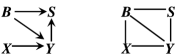
Figure 8: DAG for a matched (on $B$) case-control study (left) and moral graph (right).

In addition to collapsing over $S$, we might want to reduce dimensionality of covariates, for example, to improve stability of estimates of odds ratios (Robinson and Jewell, 1991). This is possible if the set of covariates can be written as $(B,C)$ such that $\mathit{OR}_{YX}(B,C,S)$ is collapsible over $S$ and $B$ in a way such that an estimate for $\mathit{OR}_{YX}(C,S=1)$ is consistent for $\mathit{OR}_{YX}(B,C)$. The following is straightforward from Theorem 2 and assumes that there is outcome-dependent sampling, that is, $Y\perp\!\!\!\perp\diagup\ S|(B,C,X)$ so that, unlike Corollary 4, the next corollary is not symmetric in $X$ and $Y$.

Corollary 5.

The odds ratio $\mathit{OR}_{YX}(B,C,S)$ is collapsible over $S$, over $(B,S)$ and over $B$ if $X\perp\!\!\!\perp S|(Y,B,C)$ and: [(ii)]

$X\perp\!\!\!\perp B|(Y,C)$ or

$Y\perp\!\!\!\perp B|(X,C)$ and $X\perp\!\!\!\perp S|(Y,C)$.

First note that $X\perp\!\!\!\perp S|(Y,B,C)$ yields $\mathit{OR}_{YX}(B,C,S)$ collapsible over $S$. For part (i) additionally, $X\perp\!\!\!\perp B|(Y,C)$ yields $\mathit{OR}_{YX}(B,C)$ collapsible over $B$ by Theorem 2. Both conditional independencies together imply that $X\perp\!\!\!\perp S|(Y,C)$ which finally yields $\mathit{OR}_{YX}(C,S)$ collapsible over $S$, so that all these are equal to $\mathit{OR}_{YX}(C)$. For part (ii) we see that $\mathit{OR}_{YX}(B,C)$ is collapsible over $B$ due to $Y\perp\!\!\!\perp B|(X,C)$ and we further have that $\mathit{OR}_{YX}(C,S)$ is collapsible over $S$ due to $X\perp\!\!\!\perp S|(Y,C)$. This yields the desired result.

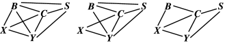
Figure 9: Illustrations of Corollary 5: left graph satisfies $X\perp\!\!\!\perp S|(Y,B,C)$, middle graph satisfies condition (i) and right graph satisfies condition (ii).

The conditions of Corollary 5 can again be checked on graphical models by corresponding separations; see Figure 9. As before, if $B$ can be appropriately partitioned, Corollary 5 can be applied successively to the subsets $B_{k}$. When DAGs are used to check Corollary 5, then the moral graph(s) have to be identical to or have fewer edges than those in Figure 9. The DAGs in Figures 3 and 5 serve as examples for the prospective and retrospective approaches, respectively. From both we infer that we can collapse over $S$, but only the second one also satisfies (i) of Corollary 5. In contrast it can be seen from Figure 3 that the conditions (i) and (ii) of Corollary 5 will not be satisfied in a DAG that represents the prospective view and where $B$ as well as $X$ point at $Y$.

3.4 Testability of the Null Hypothesis

In general data situations, for example, when $Y$ is continuous, the odds ratio is not necessarily an appropriate measure of dependence. Other measures are typically not identified under outcome-dependent sampling without further assumptions. However, a result analogous to Theorem 2 can still be obtained if we restrict ourselves to the question whether the (conditional) independence of $X$ and $Y$, possibly given covariates $C$, can still be tested under outcome-dependent sampling. This conditional independence is often the null hypothesis of interest.

Theorem 6.

If $S\perp\!\!\!\perp Y|(C,X)$ or $S\perp\!\!\!\perp X|(C,Y)$, then

$$Y\perp\!\!\!\perp X|C\quad\Longleftrightarrow\quad Y\perp\!\!\!\perp X|(C,S=1).$$

By the properties of conditional independence (Dawid, 1979) we have that $Y\perp\!\!\!\perp X|C$ together with $S\perp\!\!\!\perp Y|(C,X)$ (or $S\perp\!\!\!\perp X|(C,Y)$) immediately implies $Y\perp\!\!\!\perp X|(C,S)$. Now assume that$Y\perp\!\!\!\perp X|(C,S=1)$ and $S\perp\!\!\!\perp Y|(C,X)$; then $p(y|x,c)=\sum_{s}p(y|s,x,c)p(s|x,c)=\sum_{s}p(y|S=1,c)p(s|x,c)$which is just $p(y|S=1,c)$. If instead $S\perp\!\!\!\perp X|(C,Y)$, an analogous argument yields $p(x|y,c)=p(x|S=1,c)$. This completes the proof.

Hence, under the assumptions of Theorem 6 we can test the null hypothesis of no (conditional) association between exposure and response even under outcome-dependent sampling by any appropriate test for $Y\perp\!\!\!\perp X|(C,S=1)$. Note that $S$ has to satisfy the same conditions as for collapsibility of the odds ratio in Theorem 2; this can be explained by the one-to-one relation between (conditional) independence and vanishing mixed derivative measures of interaction (Whittaker, 1990, page 35) which are a generalization of odds ratios to continuous distributions.

3.5 Application: Hormone Replacement Therapy (HRT) and Transient Cerebral Ischemia (TCI)

We illustrate the above with a simplified version of the analysis of Pedersen et al. (1997). The data are from a case-control study, where the disease of interest is transient cerebral ischemia ($\mathit{TCI}$) and the main risk factor is use of hormone replacement therapy ($\mathit{HRT}$). Controls are matched by age. Further, smoking status ($\mathit{Smo}$), occupation ($\mathit{Occ}$) and history of other thromboembolic disorders ($\mathit{THist}$) are included. All covariates here are categorical; in particular $\mathit{HRT}$ is measured with categories “never” (the reference category), “former,” “oestrogen” and “combined.” The target of inference is the $\mathit{TCI}$–$\mathit{HRT}$ odds ratio conditional on all covariates. Under what additional assumptions this can be given a causal interpretation will be addressed explicitly in the next section.

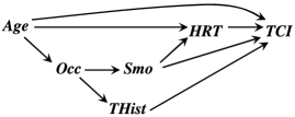
Figure 10: Prospective model for $\mathit{HRT}$–$\mathit{TCI}$ example.

Assume the conditional independencies represented in the DAG in Figure 10. The additional knowledge that the actual study design is case-control matched by age is easily included by drawing arrows from $\mathit{Age}$ and $\mathit{TCI}$ into the additional node $S$, as in Figure 11. Note that the assumptions implied by the subgraph on the covariates are supported by the data from the controls only and extrapolated to hold for the whole population.

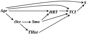
Figure 11: DAG as in Figure 10 but now including selection node $S$ to reflect matched case-control sampling.

The moral graph on all variables is shown in Figure 12. This represents the conditional independence structure that we would expect to see in the data (i.e., conditional on $S=1$). Note that a particular feature of the age matching is that $\mathit{TCI}\perp\!\!\!\perp\mathit{Age}|S=1$ but as this is not necessarily the case for $S=0$ we have to leave the edge $\mathit{TCI}$–$\mathit{Age}$ in the moral graph. (It is clear that the $\mathit{TCI}$–$\mathit{Age}$ odds ratio cannot be estimated from case-control data matched by age; formally, it is not collapsible over $S$.)

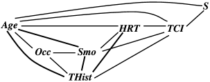
Figure 12: Moral graph on all nodes of Figure 11.

It is obvious from the moral graph as well as from the design of the study that, given $\mathit{TCI}$ and $\mathit{Age}$, all other variables are independent of the sampling indicator $S$. In particular $\mathit{HRT}\perp\!\!\!\perp S|(\mathit{TCI},\mathit{Age},\mathit{Occ},\break\mathit{Smo},\mathit{THist})$ so that Corollary 4 is satisfied, meaning that the conditional $\mathit{TCI}$–$\mathit{HRT}$ odds ratio (given all covariates) based on the selected sample is consistent for the one in the population. In addition we see that $B=\mathit{Occ}$ is independent of $\mathit{TCI}$ given $\mathit{Age}$, $\mathit{Smo}$, $\mathit{THist}$ and $\mathit{HRT}$ so that condition (ii) of Corollary 5 holds and we can ignore the occupation of a person when estimating the conditional odds ratio between $\mathit{TCI}$ and $\mathit{HRT}$.

The actual calculation of the desired odds ratio can be carried out by fitting a log-linear model on the subgraph of Figure 12 excluding the selection node $S$ (Darroch, Lauritzen and Speed, 1980; Lauritzen, 1996, Chapter 4). The desired conditional $\mathit{TCI}$–$\mathit{HRT}$ odds ratio is a function of the interaction parameters in this model. For this dataset, we obtain the log (conditional) odds ratios given in Table 1 (there is no evidence that these are different in the subgroups defined by the conditioning variables $\mathit{Age}$, $\mathit{THist}$, $\mathit{Smo}$).

Table 1: Conditional odds ratio between $\mathit{HRT}$ and $\mathit{TCI}$ given $\{\mathit{Age}$, $\mathit{THist}$, $\mathit{Smo}\}$ based on separations in the DAG of Figure 11

$\bolds{\mathit{HRT}}$ level	log-OR (stdev)	OR
Never	Reference
Former	0.64 (0.16)	1.90
Oestrogen	0.73 (0.21)	2.07
Combined	0.26 (0.19)	1.29

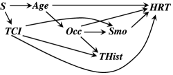
Figure 13: DAG reflecting the sampling process for the $\mathit{HRT}$–$\mathit{TCI}$ example.

Earlier we assumed that the conditional $\mathit{TCI}$–$\mathit{HRT}$ odds ratio given all other covariates is the target of interest. If for some reason instead one wants to condition only on a subset of $\{\mathit{Occ},\mathit{Smo},\mathit{THist},\break\mathit{Age}\}$, this is still collapsible over $S$ as long as $\mathit{Age}$ is included in that subset.

An alternative approach is to use a DAG that factorizes retrospectively according to the sampling process so that $S$ (and hence $\mathit{TCI}$ and $\mathit{Age}$) are the initial variables, taking into account that observations are conditional on being sampled in the first place. Assume the conditional independencies represented in the DAG in Figure 13 which is supported by the data. Collapsibility over $S$ (given the covariates) is of course still satisfied as this is implied by the design and still reflected in the model assumptions encoded by the graph.

From the moral graph in Figure 14 we now have that $\mathit{HRT}$ is conditionally independent of $\mathit{THist}$given the remaining variables so that condition (i) of Corollary 5 is satisfied with $B=\mathit{THist}$. The conditional $\mathit{TCI}$–$\mathit{HRT}$ odds ratio given $\mathit{Occ}$, $\mathit{Smo}$, $\mathit{Age}$ estimated from the case-control data is now consistent for the desired odds ratio in the target population. The results are similar to the first model as can be seen from Table 2. They are not exactly the same as the model assumptions of Figures 11 and 13 are indeed different, but they are both consistent, under their respective model, for the same odds ratio given all covariates.

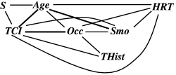
Figure 14: Moral graph for Figure 13.

Table 2: Conditional odds ratio between $\mathit{HRT}$ and $\mathit{TCI}$ given $\{\mathit{Age}$, $\mathit{Occ}$, $\mathit{Smo}\}$ based on separations in the DAG of Figure 13

$\bolds{\mathit{HRT}}$ level	log-OR (stdev)	OR
Never	Reference
Former	0.66 (0.16)	1.93
Oestrogen	0.74 (0.21)	2.10
Combined	0.28 (0.19)	1.32

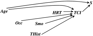
Figure 15: Graphical assumptions implicit in a logistic regression.

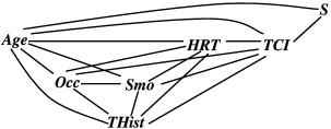
Figure 16: Moral graph for Figure 15.

A standard analysis based on a logistic regression of $\mathit{TCI}$ on explanatory variables $\mathit{Age},\mathit{Occ},\mathit{Smo},\break\mathit{THist},\mathit{HRT}$ implicitly assumes the model in Figure 15, that is, all covariates are parents of $\mathit{TCI}$. While the logistic regression does not make assumptions about the relations between the covariates, we have drawn the graph assuming they are mutually independent. This is to demonstrate that the moral graph, given in Figure 16, in any case has all covariates forming a complete subgraph, that is, there are no conditional independencies given $\mathit{TCI}$. The results can therefore be different from the above analyses, as conditional independencies involving the covariates cannot be exploited to collapse over either $\mathit{Occ}$ or $\mathit{THist}$. Adjusting for more covariates than necessary can lead to larger standard errors in logistic regressions (see Robinson and Jewell, 1991), but this happens not to be the case here; see Table 3.

In a more realistic analysis there will be more variables to be taken into account, such as menopause, other medical conditions (hypertension, diabetes,heart diseases) and body mass index (see Pedersen et al., 1997), so that logistic regression produces larger standard errors. The graphical approach based on Corollary 5 can help to reduce the set of covariates to be adjusted for.

Table 3: Conditional odds ratio between $\mathit{HRT}$ and $\mathit{TCI}$ given $\{\mathit{Age}$, $\mathit{Occ}$, $\mathit{Smo}$, $\mathit{THist}\}$ from a logistic regression

$\bolds{\mathit{HRT}}$ level	log-OR (stdev)	OR
Never	Reference
Former	0.66 (0.16)	1.93
Oestrogen	0.76 (0.21)	2.14
Combined	0.28 (0.19)	1.32

4 Causal Effects of Interventions

So far we have regarded the conditional odds ratio given all covariates as the target measure of association between $X$ and $Y$. However, in many situations one is interested in the causal effect of $X$ on $Y$, not just the association. A causal effect is meant to represent the effect that manipulations or interventions in $X$ have on $Y$, as opposed to the mere observation of different $X$ values. Hence we define the causal effect formally as the effect of an intervention. Our approach goes back to the work of Spirtes, Glymour and Scheines (1993), Pearl (1993) and is detailed in the article by Dawid (2002) (see also Lauritzen, 2000; Dawid and Didelez, 2010). We define an indicator $\sigma_{X}$ for an intervention in $X$, where $\sigma_{X}$ indicates either that $X$ is being set to a value $x\in\mathcal{X}$ in the domain of $X$, or that $X$ arises naturally. In the former case we write $\sigma_{X}=x$, $x\in\mathcal{X}$, and in the latter $\sigma_{X}=\varnothing$. More precisely,

$$p(x^{\prime}|W;\sigma_{X}=x)=\delta\{x=x^{\prime}\},$$ (5)

where $W$ can be any set of additional variables and $\delta$ is the indicator function. Hence $X$ is independent of any other variable when $\sigma_{X}=x$. In contrast, $p(x^{\prime}|W;\sigma_{X}=\varnothing)$ is the conditional distribution of $X$ given $W$ that we observe when no intervention takes place, that is, if $X$ arises naturally. More generally one may be interested in other types of interventions, for example, where (5) is a probability or depends on $W$ (Dawid and Didelez, 2010; Didelez et al., 2006), but we do not consider these in more detail here. The above approach is related to the potential outcomes framework (Rubin, 1974, 1978; Robins, 1986), in that the distribution of the outcome $Y$ under an intervention, $p(y|\sigma_{X}=x)$, corresponds to the distribution of the potential outcome $Y_{x}$. A comparison of different causal frameworks can be found in the work of Didelez and Sheehan (2007b). We also call the situation $\sigma_{X}=\varnothing$ the observational regime and the situation $\sigma_{X}=x$, for some $x\in\mathcal{X}$, the experimental or interventional regime.

4.1 Influence Diagrams and Causal DAGs

The indicator $\sigma_{X}$ must be regarded as a decision variable or parameter, not as a random variable and hence every statement about the system under investigation must be made conditional on the value of $\sigma_{X}$. We will use conditional independence statements of the type “$A$ is independent of $\sigma_{X}$ given $B$,” or $A\perp\!\!\!\perp\sigma_{X}|B$, meaning that the conditional distribution of $A$ given $B$ is the same under observation and any setting of $X$. With this notion of conditional independence applied to the intervention indicator, we can then also include $\sigma_{X}$ into our DAG representation of a data situation in order to encode which variables are conditionally independent of $\sigma_{X}$ in the above sense. As $\sigma_{X}$ is not a random variable but a decision variable it is graphically represented in a box and the resulting DAG is called an influence diagram (Dawid, 2002); cf. Figure 17 for an example.

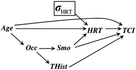
Figure 17: Influence diagram for $\mathit{TCI}$ example, prospectively.

The following points are important when constructing an influence diagram.

(1) As the decision to intervene in $X$ immediately affects its distribution, $\sigma_{X}$ has to be a graph parent of $X$, while $\sigma_{X}$ itself has no parents as it is a decision node.

(2) Hence, any variables that are nondescendants of $\sigma_{X}$ are assumed independent of $\sigma_{X}$, that is, they are not affected by an intervention in $X$. Such variables are often called “pre-treatment” or “baseline” covariates, such as age, gender, etc. Figure 17, for instance, encodes the assumption that the distribution of age, occupation, smoking status and prior thromboembolic disorders does not change if HRT is manipulated, while TCI is potentially affected. Thus, by representing variables as nondescendants or descendants of $\sigma_{X}$ we can explicitly distinguish between variables that are known a priori not to be affected by an intervention in $X$ and those that are. It is therefore not sensible to add such an intervention node to a retrospective graph such as Figure 13 as important prior knowledge about what is and is not potentially affected by an intervention in $X$ could then not be represented. Retrospective graphs encode a different set of assumptions that can be used to justify collapsibility as illustrated in Section 3.5 in order to apply condition (i) of Corollary 5, for instance.

(3) Finally, $X$ being the only child of $\sigma_{X}$ encodes the assumption that variables that are potentially affected by an intervention (i.e., descendants of $X$) are conditionally independent of $\sigma_{X}$ given ($X$, pa$(X)$). Justification of this assumption requires us to makes the system “rich” enough, often by including unobservable variables. Figure 17 assumes that $\mathit{TCI}\perp\!\!\!\perp\sigma_{\mathit{HRT}}|(\mathit{Age},\mathit{Smo},\mathit{HRT})$. This means that once we know age and smoking status of a person and, for example, that she is not taking $\mathit{HRT}$, then it does not matter in terms of predicting $\mathit{TCI}$ whether this is by choice or for instance because $\mathit{HRT}$ is banned from the market. This assumption has to be scrutinized with regard to the particular intervention that is considered and variables that are taken into account. If, for example, smoking status was unobserved and omitted from the graph, then the absence of an edge from $\sigma_{\mathit{HRT}}$ to $\mathit{TCI}$ in the new graph might not be justifiable as $\mathit{TCI}\perp\!\!\!\perp\diagup\ \sigma_{\mathit{HRT}}|(\mathit{Age},\mathit{HRT})$ if Figure 17 is correct (see moral graph in Figure 19). We might even doubt the independence $\mathit{TCI}\perp\!\!\!\perp\sigma_{\mathit{HRT}}|(\mathit{Age},\break\mathit{Smo},\mathit{HRT})$ in Figure 17, for example, if it is thought that socioeconomic background predicts $\mathit{HRT}$ and $\mathit{TCI}$ in a way not captured by $\{\mathit{Age},\mathit{Smo}\}$.

With an influence diagram constructed as above, the distribution of all variables under an intervention $\sigma_{X}=x^{\prime}$ is given by (2) with the only modification that $p(x|$pa$(x))$ is replaced by $\delta\{x=x^{\prime}\}$ due to (5). This results in the well-known intervention formula an early version of which appears in the article by Davis (1984) (see also Spirtes, Glymour and Scheines, 1993; Pearl, 1993).

We want to stress that influence diagrams are more general than causal DAGs which have become a popular tool in epidemiology (Greenland et al., 1999a). The assumptions underlying a causal DAG are equivalent to those represented in an influence diagram that has intervention nodes $\sigma_{v}$ and edges $\sigma_{v}\rightarrow v$ for every node $v\in V$ in the DAG. The absence of directed edges from $\sigma_{v}$ to any other variable than $v$ translates for a causal DAG to the requirement that all common causes of any pair of variables have to be included in the graph. Hence, readers who are more familiar with causal DAGs can think of influence diagrams as causal DAGs (ignoring $\sigma_{X}$), but they are then making stronger assumptions. For a critical view on causal DAGs see the article by Dawid (2010).

4.2 Population Causal Effect

We give two definitions of causal effects that are relevant for the present article. They are in the spirit of similar definitions in the literature (Rubin, 1974; Robins, 1986; Pearl, 2000; Dawid, 2002). We formulate them first in terms of distribution and later specify particular causal parameters.

A population causal effect is some contrast between the post-intervention distributions $p(y|\sigma_{X}=x)$, $x\in\mathcal{X}$, of $Y$ for different interventions, for example, setting $X$ to $x_{1}$ as opposed to $x_{2}$. One could say that this is a valid target of inference if we contemplate administering a treatment to the whole population. Most radically one can say that $X$ has a causal effect on $Y$ if for some values $x_{1}\not=x_{2}\in\mathcal{X}$ the two distributions $p(y|\sigma_{X}=x_{i})$, $i=1,2$, differ in some aspect. If one can estimate these post-intervention distributions from observable data, then one can estimate any contrast between them. When $p(y|\sigma_{X}=x)\not=p(y|X=x;\sigma_{X}=\varnothing)$ we say that the effect of $X$ on $Y$ is (marginally) confounded. [Note that as detailed by Greenland, Pearl and Robins (1999b) it is important to treat confounding and noncollapsibility as distinct concepts.] We can adjust for confounding if a set of variables $C$ is observed satisfying the following conditions (4.2) and (7) [in short we call this a sufficient set of covariates (Dawid, 2002)]. Assume we know that $Y\perp\!\!\!\perp\sigma_{X}|(X,C)$, that is,

$$p(y|C=c;\sigma_{X}=x)$$

(6)

$$\quad=p(y|X=x,C=c;\sigma_{X}=\varnothing),$$

meaning that once we know $C$ and the value $x$, then it does not make a difference whether $X=x$ has been observed to happen by nature or by intervention. If in addition

$$C\perp\!\!\!\perp\sigma_{X},$$ (7)

that is, the covariates $C$ are pre-treatment, then the post-intervention distribution can be consistently estimated from prospective data (provided $C$ is observed). The post-intervention distribution for setting $X$ to $x$ is obtained as

$$p(y|\sigma_{X}=x)$$

$$\quad=\sum_{x^{\prime},c}p(y|c,x^{\prime};\sigma_{X}=x)p(x^{\prime}|c;\sigma_{X}=x)p(c)$$

(8)

$$\quad=\sum_{x^{\prime},c}p(y|c,x^{\prime};\sigma_{X}=\varnothing)\delta\{x=x^{\prime}\}p(c)$$

$$\quad=\sum_{c}p(y|c,x;\sigma_{X}=\varnothing)p(c),$$

where the last step is due to (5). The quantities $p(y|c,x;\sigma_{X}=\varnothing)$ and $p(c)$ can be consistently estimated from prospective data on $X,Y$ and $C$. As pointed out, for example, by Clayton (2002), (4.2) corresponds to classical direct standardization. The above conditions (4.2) and (7) are equivalent to Pearl’s (1995, 2000) so-called back-door criterion for causal graphs (Lauritzen, 2000). If we cannot find a set of covariates that satisfies (4.2) and (7), an alternative is to use an instrumental variable, but we do not consider this any further here (see Angrist, Imbens and Rubin 1996; Didelez and Sheehan, 2007a).

Consider again Figure 17. We can see that $C=\{\mathit{Age}$, $\mathit{Occ}$, $\mathit{Smo}$, $\mathit{THist}\}$ satisfies (4.2) and (7). But these properties are also satisfied for the smaller set $C^{\prime}=\{\mathit{Age},\mathit{Smo}\}$. $\mathit{Age}$ and $\mathit{Smo}$ are independent of $\sigma_{\mathit{HRT}}$, as can be seen from the moral graph in Figure 18, and together with $\mathit{HRT}$ they separate $Y$ and $\sigma_{\mathit{HRT}}$ as can be seen from the second moral graph in Figure 19. This implies that in a prospective study we can ignore $\mathit{Occ}$ and $\mathit{THist}$ altogether and apply (4.2) to obtain the post-intervention distribution.

If, instead, we were to investigate the causal effect of smoking on $\mathit{TCI}$ we might assume an influence diagram as in Figure 20 (ignoring $S$). We can see by a similar reasoning that $C=\{\mathit{Occ}\}$ is a sufficient set of covariates. Note that, in this case, the mediating variable $\mathit{HRT}$ must not be included in $C$ as it does not satisfy (7). This illustrates that the population causal effect that is identified by conditions (4.2) and (7) is an overall or total effect, for example, the effect of smoking on $\mathit{TCI}$ as potentially mediated by its effect on $\mathit{HRT}$.

As can be seen from (4.2), the population causal effect depends on the distribution of $C$ in the population; this is not always desirable as it may mean that we cannot carry forward the results to another population. Hence we consider the conditional causal effect next.

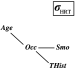
Figure 18: Moral graph on $\mathit{Age}$, $\mathit{Occ}$, $\mathit{Smo}$, $\mathit{THist}$ and $\sigma$ for Figure 17.

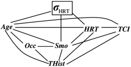
Figure 19: Moral graph on all variables for Figure 17.

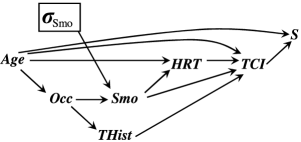
Figure 20: Influence diagram for $\mathit{TCI}$ example with intervention in ‘smoking.’

4.3 Conditional Causal Effects

A conditional causal effect is some contrast between the post-intervention distributions conditional on some covariates $C$, $p(y|C;\sigma_{X}=x)$, $x\in\mathcal{X}$ (for the moment $C$ need not be the same as in (4.2), but we get back to this). Such a conditional causal effect may be of interest if one wants to measure how effective treatment is for a particular patient with known characteristics such as gender, medical history, etc. It therefore seems reasonable to assume that these covariates $C$ satisfy (7). We further assume that they also satisfy (4.2) because otherwise we would need to take additional suitable covariates into account in order to apply (4.2), so we might as well incorporate them immediately. Also, if $C$ satisfies both properties, the conditional causal effect does not depend on the population distribution of covariates. With (4.2) and (7) the conditional post-intervention distribution is automatically identified if $C$ is observed. Note that in order to obtain the population causal effect using (4.2) we can choose any set $C$ such that (4.2) and (7) are satisfied, whereas when we consider the conditional causal effect $C$ could include more variables, for example, because they are so-called effect modifiers. For example, in Figure 17 one may be interested in the conditional causal effect given $\mathit{Age}$, $\mathit{Smo}$ and $\mathit{THist}$ if the latter is thought to predict a different effect of $\mathit{HRT}$ on $\mathit{TCI}$, even though it is not necessary to adjust for $\mathit{THist}$ to obtain the population causal effect.

As alluded to earlier, both the population but also the conditional causal effect are “total” causal effects, when $C$ satisfies (7), in the sense that they include direct as well as indirect effects of $X$ on $Y$; for example, the effect of smoking on $\mathit{TCI}$ may be moderated by $\mathit{HRT}$. A detailed treatment of this topic is beyond the scope of this article but we refer to the works of Pearl (2001), Robins (2003) and Didelez, Dawid and Geneletti (2006) and Geneletti (2007) for the general theory, and conditions of identifiability, of direct and indirect effects especially in the nonlinear case.

4.4 Inference on Causal Effect

We review testing for the causal effect based on prospective data. In the broadest sense, the causal null hypothesis is that the post-intervention distribution of $Y$, $p(y|\sigma_{X}=x)$ (or possibly $p(y|c;\sigma_{X}=x)$ if we consider the conditional causal effect), does not depend on the value $x$, that is, we do not change the distribution of $Y$ by setting $X$ to different values. It is clear from (4.2) that if there is no conditional causal effect, that is, if $Y\perp\!\!\!\perp X|(C;\sigma_{X}=\varnothing)$, then there is also no population causal effect. The converse is not necessarily true, in particular when there are different effects in different subgroups that may happen to cancel each other out such that there is no overall effect in the whole population, that is, $p(y|\sigma_{X}=x)$ is independent of $x$ without $Y\perp\!\!\!\perp X|(C;\sigma_{X}=\varnothing)$ being true—this is known as lack of faithfulness (see Spirtes, Glymour and Scheines, 1993). Hence we suggest testing $Y\perp\!\!\!\perp X|(C;\sigma_{X}=\varnothing)$ in order to investigate the causal null hypothesis of no (conditional) causal effect. If this independence can be rejected, then there is evidence for a conditional causal effect, and (except in rare cases of such lack of faithfulness) for a population effect.

For estimation, we need to define the causal parameter of interest. Much of the causal literature is based on the difference in expectation, leading to the average population and average conditional causal effect, $E(Y|\sigma_{X}=x_{1})-E(Y|\sigma_{X}=x_{2})$ (often denoted by $ACE$) and $E(Y|C=c;\sigma_{X}=x_{1})-E(Y|C=c;\sigma_{X}=x_{2})$, respectively.

Here, we focus instead on population and conditional causal odds ratios as these are invariant to the marginal distributions and hence applicable under outcome-dependent sampling, as will be seen. Assume that $Y$ and $X$ are binary. The population causal odds ratio ($\mathit{COR}$) is defined as

$$\mathit{COR}_{YX}=\frac{p(Y=1|\sigma_{X}=1)p(Y=0|\sigma_{X}=0)}{p(Y=0|\sigma_{X}=1)p(Y=1|\sigma_{X}=0)}.$$

Alternatively consider the conditional $\mathit{COR}_{YX}(C=c)$ where we condition on the set of covariates $C=c$, that is,

$$\mathit{COR}_{YX}(C=c)$$

$$\quad=\frac{p(Y=1|c;\sigma_{X}=1)p(Y=0|c;\sigma_{X}=0)}{p(Y=0|c;\sigma_{X}=1)p(Y=1|c;\sigma_{X}=0)}.$$

This is distinct from the population $\mathit{COR}_{YX}$ when it is not collapsible over $C$, just as for the associational odds ratio. When a set of covariates $C$ is sufficient to adjust for confounding, that is, satisfies (4.2) and (7), then $p(Y=1|c;\sigma_{X}=x)=p(Y=1|c,X=x;\sigma_{X}=\varnothing)$ and hence $\mathit{COR}_{YX}(C)=\mathit{OR}_{YX}(C)$. This means we can use Corollary 3 in order to check whether $C$ can be reduced, that is, whether $\mathit{OR}_{YX}(C)$ and hence $\mathit{COR}_{YX}(C)$ is collapsible over a subset of $C$.

4.5 Causal Inference in Case-Control Studies

Now we include the sampling variable $S$ in our considerations. Note that the targeted causal parameters do not involve $S$, so we only want to make assumptions about the distribution of $S$ under the observational regime $\sigma_{X}=\varnothing$. In the simple situation of a case-control study (without matching) sampling is just on the values of $Y$. Therefore we assume that

$$S\perp\!\!\!\perp(C,X)|(Y;\sigma_{X}=\varnothing)$$ (9)

and in addition (4.2) and (7). These together imply the following factorization:

$$p(y,c,x,s|\sigma_{X}=\varnothing)$$

$$\quad=p(s|y;\sigma_{X}=\varnothing)p(y|c,x)$$ (10)

$${}\qquad\times p(x|c;\sigma_{X}=\varnothing)p(c).$$

The influence diagram in Figure 21 represents slightly stronger restrictions, as it implies $S\perp\!\!\!\perp\sigma_{X}|Y$ which does not follow from (4.2), (7) and (9); that is, we do not specify any assumptions about the distribution of $S$ under $\sigma_{X}=x$ as this is not relevant to the target of inference. We will nevertheless use influence diagrams like Figure 21 to represent jointly our assumptions about the sampling process and the contemplated intervention.

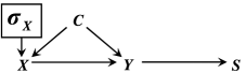
Figure 21: DAG representing simple case-control situation.

The data come from the distribution $p(y,c,x|S=1;\sigma_{X}=\varnothing)$, given by

$$\frac{p(S=1|y)p(y|c,x)p(x|c;\sigma_{X}=\varnothing)p(c)}{p(S=1|\sigma_{X}=\varnothing)},$$ (11)

similar to (2.4). The moral graph in Figure 22 includes an edge between $\sigma_{X}$ and $C$ as the conditional distribution of $C$ given $S$ is not the same for different regimes $\sigma_{X}$. Hence if individuals are selected based on their case or control status, we cannot expect the distribution of the covariates to be the same in a scenario where the risk factor $X$ has been manipulated by external intervention as in a scenario where it has been left to arise naturally.

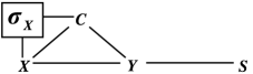
Figure 22: Moral graph for simple case-control situation.

The following theorem revisits the well-known result that the causal effect of $X$ on $Y$ can be tested, and the causal odds ratio estimated, from case-control data (Breslow, 1996). The target of inference is$\mathit{COR}_{YX}(C)$, based on $p(y|c;\sigma_{X}=x)$, which is prospective in the sense that we want to predict the effect of manipulating $X$ on $Y$ after knowing $C$ without conditioning on $S$ while we have only the retrospective information $p(y|c,S=1;\sigma_{X}=\varnothing)$ available. The following theorem allows $S$ to depend on the covariates $C$ as well as on $Y$.

Theorem 7.

Under (4.2), (7) and assuming $S\perp\!\!\!\perp X|(C,Y;\sigma_{X}=\varnothing)$, we can (i) test the null hypothesis of no conditional causal effect of $X$ on $Y$ given $C$ by testing $X\perp\!\!\!\perp Y|(C,S=1;\sigma_{X}=\varnothing)$ (regardless of the measurement scales), and (ii) consistently estimate $\mathit{COR}_{YX}(C)$ by estimating $\mathit{OR}_{YX}(C,S=1)$ (for categorical $X,Y$).

(i) Earlier we argued that a test for$Y\perp\!\!\!\perp X|(C;\sigma=\varnothing)$ can replace a test of the null hypothesis of no causal effect when $C$ satisfies (4.2) and (7). As $S\perp\!\!\!\perp X|(C,Y;\sigma_{X}=\varnothing)$, Theorem 6 completes the argument.

(ii) Assumptions (4.2) and (7) imply $\mathit{COR}_{YX}(C)=\mathit{OR}_{YX}(C)$ as explained earlier. With Corollary 4 we see that $\mathit{OR}_{YX}(C,S)$ is collapsible over $S$ when $S\perp\!\!\!\perp\break X|(C,Y;\sigma_{X}=\varnothing)$, which completes the proof.

In Theorem 7, as far as testing is concerned, we are not restricted to the categorical situation and can use as test statistic whatever seems appropriate given the measurement scales of $X,Y,C$. If this independence is rejected, then there is evidence for a causal effect. In the particular case of binary $Y$ and continuous $X$ it is well known that we can still also consistently estimate the odds ratio using a logistic regression (Prentice and Pyke, 1979). Their result, however, relies on the logistic link being justified, while the results on odds ratios when $X$ and $Y$ are both categorical, such as Theorem 7(ii), make no parametric assumptions.

The set $C$ in Theorem 7 needs to contain a sufficient set of covariates so as to justify (4.2). But it also needs to contain any matching variables, even if these are not needed for (4.2), in order to justify $S\perp\!\!\!\perp X|(C,Y;\sigma_{X}=\varnothing)$. This has been illustrated in Figure 8, with the variable $B$ which is not needed to adjust for confounding. Hence, a sufficient set of covariates and the matching variables are required for Theorem 7 to work. However, typically a much larger set of covariates has been observed; one can then use Corollary 5 to reduce it without losing information, as in the following example.

In the $\mathit{HRT}$–$\mathit{TCI}$ example, as the study design was case-control matched by $\mathit{Age}$, we need to make sure that $C$ contains $\mathit{Age}$. But we already saw that $C=\{\mathit{Age},\mathit{Smo}\}$ is a set of sufficient covariates. Hence, all assumptions of Theorem 7 are satisfied with this choice of $C$ (check these on the influence diagram in Figure 23). That is, we can consistently estimate the causal odds ratio between $\mathit{HRT}$ and $\mathit{TCI}$ given $\mathit{Age},\mathit{Smo}$ from the available data.

Alternatively, if the target is the conditional causal odds ratio given all covariates, then we can see that with the choice of $C^{\prime}=\{\mathit{Age},\mathit{Occ},\mathit{THist},\mathit{Smo}\}$ the conditions of Theorem 7 are satisfied; we can estimate the causal odds ratio $\mathit{HRT}$ and $\mathit{TCI}$ given $C^{\prime}$ from the available data, but we can additionally omit $\mathit{Occ}$ due to the conditional odds ratio being collapsible over this variable. Note that it is not further collapsible over the variable $\mathit{THist}$, implying that the causal odds ratio given $C=\{\mathit{Age},\mathit{Smo}\}$ is different from the causal odds ratio given $C^{\prime}=\{\mathit{Age},\mathit{Occ},\mathit{THist},\mathit{Smo}\}$, though both conditioning sets are sufficient to adjust for confounding under our assumptions. As mentioned before, $\mathit{THist}$ could be an effect modifier and might therefore be included.

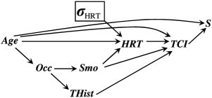
Figure 23: Influence diagram for $\mathit{TCI}$ example with matched sampling.

Table 4: Conditional causal odds ratio between $\mathit{Smo}$ and $\mathit{TCI}$ given ($\mathit{Age}$, $\mathit{THist}$)

Smoking level	log-OR (stdev)	OR
Never	Reference
Former	0.41 (0.21)	1.51
1–10	0.89 (0.19)	2.43
11–20	0.97 (0.18)	2.65
21$+$	1.19 (0.41)	3.29

Assume now that we are instead interested in the effect of smoking ($\mathit{Smo}$) on $\mathit{TCI}$ and that the assumptions encoded in Figure 20 are satisfied. So far we have targeted the conditional causal odds ratio between exposure and response given all covariates; however, if we include the mediator $\mathit{HRT}$ into $C$, then it does not satisfy condition (7) as it is a descendant of $\mathit{Smo}$. Hence we could consider $C=\{\mathit{Age}$, $\mathit{Occ}$, $\mathit{THist}\}$ and find that $\mathit{OR}_{\mathit{Smo},\mathit{TCI}}(C,S)$ can again be collapsed over $\mathit{Occ}$. The resulting estimates are shown in Table 4. Note that these describe the “total” effect of $\mathit{Smo}$ on $\mathit{TCI}$ including possible mediation via $\mathit{HRT}$ (but conditional on $\mathit{Age}$ and $\mathit{THist}$).

5 Extensions and further examples

In this section we consider more general data situations where the sampling depends in a less obvious way on the outcome and possibly on further variables. In particular, we extend the previous results to the case where a sufficient set of covariates (and possibly matching variables) $C$ does not allow us to collapse over $S$. In such cases taking further variables into account can sometimes provide a solution. Let us start with an example.

Weinberg, Baird and Rowland (1993) and Slama et al. (2006) considered ‘time-to-pregnancy’ studies which are of interest when investigating factors affecting fertility. Typically $X$ is exposure, such as a toxic substance or smoking, and $Y$ is the time to pregnancy; common covariates $C$ such as age, socioeconomic background, etc., may be taken into account. The problem here is that if women are sampled who became pregnant during a certain time interval (retrospective sampling), then long duration to pregnancy automatically means earlier initiation time. However, initiation time might predict the exposure if it has changed over time, for example, because precautions regarding toxic substances have increased or smoking habits in the population have changed over time. Therefore, $Y$ and $X$ may be associated given $C$ even if there is no causal effect of exposure, that is, $C$ is not “bias-breaking.” Note that the same phenomenon also occurs with current duration designs and that prospective sampling has many other drawbacks in “time-to-pregnancy” studies as discussed in detail by Slama et al. (2006).

The key to solving this problem is to find a bias-breaking variable $Z$ such that either $X$ or $Y$ can reasonably be assumed conditionally independent of $S$ given $Z$ (and observed covariates) and to use Corollary 3 so as to further collapse over $Z$. The method proposed by Weinberg, Baird and Rowland (1993) relies on using the time of initiation. It seems plausible that once the initiation time $Z$ and time to pregnancy $Y$ are known, the sampling $S$ is not further associated with the exposure $X$, typically controlling for relevant covariates $C$, that is, $S\perp\!\!\!\perp X|(Z,Y,C)$. Further, we may sometimes be able to justify that $Y\perp\!\!\!\perp Z|(X,C)$, that is, that the initiation time itself, once we account for relevant factors and regardless of whether the unit is sampled or not, should not predict time to pregnancy. This assumption might be violated if there are other relevant factors that have changed over time and that are not captured by $C$ or $X$.

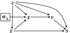
Figure 24: Graphical representation of assumption in time-to-pregnancy example.

Using again $\sigma_{X}$ as intervention indicator and assuming that $C$ is a sufficient set of covariates, we can summarize our assumptions about the time-to-pregnancy example through the following independencies: $Z\perp\!\!\!\perp\sigma_{X}$, $Y\perp\!\!\!\perp(Z,\sigma_{X})|(X,C)$ and $S\perp\!\!\!\perp\break(X,\sigma_{X})|(Z,Y,C)$. The graph in Figure 24 represents these conditional independence assumptions (the edge $C\rightarrow Z$ could be replaced by $C\leftarrow Z$). If it were not for the retrospective sampling, the causal effect of $X$ on $Y$ could be analyzed ignoring $Z$, as $C$ is assumed a sufficient set of covariates. The selection effect becomes apparent when checking for graph separation, which yields a moral edge between $Z$ and $Y$ when conditioning on $S$ (cf. moral graph in Figure 26).

The following theorem shows that exploiting the initiation time $Z$ in the above example can indeed facilitate inference about the causal effect.

Theorem 8.

We can test for a (conditional) causal effect of $X$ on $Y$ (given $C$) if there exists a set of observable variables $Z$ such that all following conditions are satisfied: [(iii)]

$S\perp\!\!\!\perp X|(Y,Z,C;\sigma_{X}=\varnothing)$,

$Y\perp\!\!\!\perp Z|(X,C;\sigma_{X}=\varnothing)$,

$C$ is a sufficient set of covariates,

the joint distribution $p(y,x,z|\sigma_{X}=\varnothing)$ is strictly positive. The causal null hypothesis is then equivalent to $Y\perp\!\!\!\perp X|(Z,C,S=1;\sigma_{X}=\varnothing)$.

As argued before, testing $Y\perp\!\!\!\perp X|(C;\break\sigma_{X}=\varnothing)$ provides a test for the causal null hypothesis. We show that it is equivalent to $Y\perp\!\!\!\perp X|(Z,C,S=1;\sigma_{X}=\varnothing)$. As all conditional independencies are conditional on $\sigma_{X}=\varnothing$ it will be omitted from the notation.

Remember that with (i) and Theorem 6, $Y\perp\!\!\!\perp X|(Z,C)$ is equivalent to $Y\perp\!\!\!\perp X|(Z,C,S=1)$. First assume that $Y\perp\!\!\!\perp X|C$. With (ii) we obtain $Y\perp\!\!\!\perp X|(Z,C)$, which is equivalent to $Y\perp\!\!\!\perp X|(Z,C,S=1)$. For the converse, assume $Y\perp\!\!\!\perp X|(Z,C,S=1)$, hence $Y\perp\!\!\!\perp X|(Z,C)$. Now, (iv) is sufficient to ensure (Lauritzen, 1996, page 29) that this conditional independence together with (ii) yields $Y\perp\!\!\!\perp(X,Z)|C$ which implies $Y\perp\!\!\!\perp X|C$.

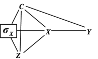
Figure 25: Moral graph for DAG in Figure 24 marginal over $S$.

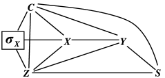
Figure 26: Moral graphs for the DAG in Figure 24 including $S$.

Consider again the time-to-pregnancy study represented in Figure 24. We see that all assumptions of Theorem 8 are satisfied: $C$ and $\sigma$ are nondescendants of each other and have no parents; from the moral graph on $Y,Z,X,C$ (Figure 25) it follows that $C$ is a sufficient set of covariates, and that (ii) holds, while part (i) can be seen from the moral graph on all nodes in Figure 26. Hence we can investigate the null hypothesis of no causal effect by testing whether $Y$ and $X$ are associated conditionally on $Z$ and $C$ for the sampled subjects.

(a) Theorem 8 is symmetric in $X,Y$, in the sense that they can be swapped in (i) and (ii).

(b) If $Z=\varnothing$, the conditions are the same as for the matched case-control situation of Section 4.5 (Theorem 7).

(c) Further, the theorem does not require that$Z\perp\!\!\!\perp\sigma_{X}$, that is, that the bias-breaking variable $Z$ is not affected by an intervention in $X$, hence in Figure 24 the arrow from $Z$ to $X$ could be reversed (though this is not plausible in the time-to-pregnancy scenario that we have used, but may be relevant in other scenarios).

It is easy to find realistic examples where the assumptions of Theorem 8 are not satisfied; for example, Robins (2001) explained why it is difficult to identify the effect of hormone treatment on endometrial cancer in case-control studies. In such situations, additional outside information can sometimes be used to obtain identifiability (see, e.g., Geneletti, Richardson and Best, 2009).

In addition to the above result about testing the causal effect, we also have the following about estimating it when all variables are discrete.

Theorem 9.

Under the assumptions of Theorem 8, we can consistently estimate the (conditional) causal odds ratio of $X$ on $Y$ given $C$, $\mathit{COR}_{YX}(C)$, by estimating $\mathit{OR}_{YX}(Z,C,S=1)$.

From (iii) it follows that $\mathit{COR}_{YX}(C)=\mathit{OR}_{YX}(C)$, that is, the causal odds ratio is equal to the observational odds ratio. Further, using Corollary 3 with $B_{1}=S$ and $B_{2}=Z$, (i) yields $\mathit{OR}_{YX}(Z,\break C,S)$ is collapsible over $S$ in the observational regime and (ii) means $\mathit{OR}_{YX}(Z,C)$ is collapsible over $Z$, hence $\mathit{OR}_{YX}(Z,C,S)$ is collapsible over $(Z,S)$.

(a) In the situation of Theorem 9 it does not necessarily hold that $\mathit{OR}_{YX}(C,S=1)=\mathit{OR}_{YX}(C)$, that is, Corollary 5 (with $B=Z$) does not apply as neither part (i) nor part (ii) of that corollary is satisfied. However, Corollary 5 can be used to further reduce the set $C$ if $\mathit{OR}_{YX}(C)$ is collapsible over a subset of $C$. The difference between the above Theorem 9 and Corollary 5 is that while the latter focuses on such a reduction of dimensionality, the former exploits the fact that $\mathit{OR}_{YX}(C)$ is the same in a higher dimensional model $\mathit{OR}_{YX}(C,\break Z,S=1)$. This is useful because we can onlyestimate quantities conditional on $S=1$ while$\mathit{OR}_{YX}(C)\not=\mathit{OR}_{YX}(C,S=1)$.

(b) Theorem 9 implies that the assumptions of Theorem 8 can be tested to a certain extent as they imply that $\mathit{OR}_{YX}(Z=z,C,S=1)=\mathit{OR}_{YX}(Z=z^{\prime},\break C,S=1)$ for $z\not=z^{\prime}$. Hence, estimates should not vary much for different values of $Z$.

We conclude with an example for potential selection bias that is not due to outcome-dependent sampling but is also covered by the conditions of Theorem 9 due to their symmetry in $X$ and $Y$.

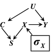
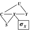
(a)	(b)
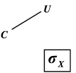
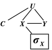
(c)	(d)

Figure 27: (a) DAG and relevant moral graphs for Hernan, Hernández-Díaz and Robins (2004) example; (b) is moral graph on all variables, (c) on $C$ and $\sigma_{X}$, (d) on $Y,X,C$ and $\sigma_{X}$.

Hernan, Hernández-Díaz and Robins (2004) considered the example illustrated in Figure 27. In a study with HIV patients $X$ is anti-retroviral therapy, $Y$ is AIDS, $U$ is the true level of immunosupression and $C$ is a collection of symptoms as well as measurements on CD4 counts. Further covariates would typically be included but for simplicity we omit them here. We assume $X$ is randomized so it has no graph parents. The fact that $S$ depends on $C$ and $X$ represents that patients with worse symptoms and side effects, predicted by treatment and baseline covariates, are more likely to drop out and not be available for the analysis. (Note that if it was not for having to condition on $S=1$, then we could estimate the population causal effect of $X$ on $Y$ without further adjustment.) We can verify that the odds ratio between $X$ and $Y$ is not collapsible over $S$ from Figure 27(b): neither $X\perp\!\!\!\perp S$ nor $Y\perp\!\!\!\perp S$. However, if we consider the conditional causal effect of $X$ on $Y$ given $C$, then we can collapse over $S$. With $Z=\varnothing$, all conditions of Theorem 9 with $X$ and $Y$ interchanged are satisfied, so we can estimate $\mathit{COR}_{YX}(C)$ by using $\mathit{COR}_{YX}(C,S=1)$; condition (i) can be seen from the moral graph in Figure 27(b), condition (ii) is redundant, condition (iii) can be seen from Figure 27(c) and (d).

6 Conclusion

As the sampling or selection mechanism can often create complications and bias in statistical analyses, we argued in Section 2.4 that the basic assumptions about the sampling, in terms of conditional independence, should be made explicit using graphical models including a node for the binary sampling indicator. We demonstrated how this allows us to characterize, with simple graphical rules, situations in which we can collapse the (conditional) odds ratio over $S$ (Corollary 4) or, more generally, when we can test for a (conditional) association (Theorem 6). Addressing specifically causal inference, Theorem 7 specifies the additional assumptions required to test for a causal effect or estimate a (conditional) causal odds ratio under outcome-dependent sampling, such as in a matched case-control design. Theorems 8 and 9 extend these results to more general situations with less obvious outcome-dependent sampling. Our results are therefore relevant to a range of study designs, case-control being the most common, but also, for example, retrospective sampling that is conditional on reaching a certain state, such as time-to-pregnancy studies.

We have shown how different types of graphical models can be used to express assumptions about the sampling process, admitting more flexibility than if restricted to causal DAGs (but as explained in Section 4.1 our results are also valid for the latter). In addition to directed acyclic and undirected graphs, we want to point out that chain graphs provide a further class of useful models. The original analysis of the $\mathit{TCI}$ data, for instance, used chain graphs (Pedersen et al., 1997). The causal interpretation of chain graphs, however, is more complicated than for DAGs (cf. Lauritzen and Richardson, 2002).

As any type of graph only encodes presence or absence of conditional independencies, it cannot represent particular parametric assumptions or properties of the model and selection process. Consequently, any inference other than testing or estimating odds ratios will typically require such additional assumptions, which in turn will need to be scrutinized and complemented by a sensitivity analysis. We therefore regard the use of graphical models in this context as an important first step of the analysis, facilitating the structuring and reasoning about the problem of outcome-dependent sampling.

Concerning the question of causal inference, we have mainly assumed an approach of adjusting for confounding by conditioning on suitable covariates in the analysis. A different way of using covariates is via the propensity score (Rosenbaum and Rubin, 1983) or inverse probability weighting (Robins, Hernan and Brumback, 2000), but little is known as yet on how to adapt these to case-control studies or general outcome-dependent sampling; but see the work of Robins, Rotnitzky and Zhao (1994, Section 6.3), Newman (2006), Mansson et al. (2007) and van der Laan (2008).

References

- (1) Altham, P. M. E. (1970). The measurement of association of rows and columns for an rs contingency table. J. Roy. Statist. Soc. Ser. B 32 63–73.
- (2) Angrist, J. D., Imbens, G. W. and Rubin, D. B. (1996). Identification of causal effects using instrumental variables. J. Amer. Statist. Assoc. 91 444–455.
- (3) Asmussen, S. and Edwards, D. (1983). Collapsibility and response variables in contingency tables. Biometrika 70 566–578. \MR0725370
- (4) Berkson, J. (1946). Limitations of the application of fourfold table analysis to hospital data. Biometrics Bull. 2 47–53.
- (5) Breslow, N. E. (1996). Statistics in epidemiology: The case-control study. J. Amer. Statist. Assoc. 91 14–28. \MR1394064
- (6) Bishop, Y. M., Fienberg, S. and Holland, P. (1975). Discrete Multivariate Analysis. MIT Press, Cambridge, MA. \MR0381130
- (7) Cooper, G. F. (1995). Causal discovery from data in the presence of selection bias. Preliminary Papers of the 5th International Workshop on Artificial Intelligence and Statistics.
- (8) Copas, J. B. and Li, H. G. (1997). Inference for non-random samples (with discussion). J. Roy. Statist. Soc. Ser. B 59 55–95. \MR1436555
- (9) Cox, D. R. and Wermuth, N. (1996). Multivariate Depencencies—Models, Analysis and Interpretation. Chapman and Hall, London. \MR1456990
- (10) Clayton, D. G. (2002). Models, parameters, and confounding in epidemiology. Invited Lecture, International Biometric Conference, Freiburg. Available at http://www-gene.cimr.cam.ac.uk/clayton/talks/ibc02.pdf.
- (11) Darroch, J. N., Lauritzen, S. L. and Speed, T. P. (1980). Markov fields and log linear models for contingency tables. Ann. Statist. 8 522–539. \MR0568718
- (12) Davis, J. A. (1984). Extending Rosenberg’s technique for standardizing percentage tables. Social Forces 62 679–708.
- (13) Davis, L. J. (1986). Whittemore’s notion of collapsibility in multidimensional contingency tables. Comm. Statist. Theory Methods 15 2541–2554. \MR0853027
- (14) Dawid, A. P. (1979). Conditional independence in statistical theory (with discussion). J. Roy. Statist. Soc. Ser. B 41 1–31. \MR0535541
- (15) Dawid, A. P. (2002). Influence diagrams for causal modelling and inference. Int. Statist. Rev. 70 161–189.
- (16) Dawid, A. P. (2010). Beware of the DAG! J. Mach. Learn. 6 59–86.
- (17) Dawid, A. P. and Didelez, V. (2010). Identifying the consequences of dynamic treatment strategies. A decision-theoretic overview. Statist. Surveys. To appear.
- (18) Didelez, V., Dawid, A. P. and Geneletti, S. (2006). Direct and indirect effects of sequential treatments. In Proceedings 22nd Conference on Uncertainty in Artificial Intelligence (R. Dechter and T. S. Richardson, eds.) 138–146. AUAI Press, Arlington, TX.
- (19) Didelez, V. and Edwards, D. (2004). Collapsibility of graphical CG-regression models. Scand. J. Statist. 31 535–551. \MR2101538
- (20) Didelez, V. and Sheehan, N. (2007a). Mendelian randomisation as an instrumental variable approach to causal inference. Statist. Meth. Med. Res. 16 309–330. \MR2395652
- (21) Didelez, V. and Sheehan, N. (2007b). Mendelian randomisation: Why epidemiology needs a formal language for causality. In Causality and Probability in the Sciences (F. Russo and J. Williamson, eds.) 263–292. College Publications, London.
- (22) Ducharme, G. R. and Lepage, Y. (1986). Testing collapsibility in contingency tables. J. Roy. Statist. Soc. Ser. B 48 197–205. \MR0867997
- (23) Edwards, A. W. F. (1963). The measure of association in a 22 table. J. Roy. Statist. Soc. Ser. A 126 109–114.
- (24) Frydenberg, M. (1990). The chain graph Markov property. Scand. J. Statist. 17 333–353. \MR1096723
- (25) Geneletti, S. (2007). Identifying direct and indirect effects in a non-counterfactual framework. J. Roy. Statist. Soc. Ser. B 69 199–215. \MR2325272
- (26) Geneletti, S., Richardson, S. and Best, N. (2009). Adjusting for selection bias in retrospective case-control studies. Biostatistics 10 17–31.
- (27) Geng, Z. (1992). Collapsibility of relative risk in contingency tables with a response variable. J. Roy. Statist. Soc. Ser. B 54 585–593. \MR1160484
- (28) Greenland, S. (2003). Quantifying biases in causal models: Classical confounding vs. collider-stratification bias. Epidemiology 14 300–306.
- (29) Greenland, S., Pearl, J. and Robins, J. M. (1999a). Causal diagrams for epidemiologic research. Epidemiology 10 37–48.
- (30) Greenland, S., Pearl, J. and Robins, J. M. (1999b). Confounding and collapsibility in causal inference. Statist. Sci. 14 29–46.
- (31) Guo, J., Geng, Z. and Fung, W.-K. (2001). Consecutive collapsibility of odds ratios over an ordinal background variable. J. Multivariate Anal. 79 89–98. \MR1867256
- (32) Heckman, J. J. (1979). Sample selection bias as a specification error. Econometrica 47 153–161. \MR0518832
- (33) Hernán, M. A., Hernández-Díaz, S. and Robins, J. M. (2004). A structural approach to selection bias. Epidemiology 15 615–625.
- (34) Kim, S.-H. and Kim, S.-H. (2006). A note on collapsibility in DAG models of contingency tables. Scand. J. Statist. 33 575–590. \MR2298066
- (35) Kreiner, S. (1987). Analysis of multidimensional contingency tables by exact methods. Scand. J. Statist. 14 97–112. \MR0913255
- (36) Lauritzen, S. L. (1982). Lectures on Contingency Tables. Aalborg Univ. Press.
- (37) Lauritzen, S. L. (1996). Graphical Models. Clarendon Press, Oxford. \MR1419991
- (38) Lauritzen, S. L. (2000). Causal inference from graphical models. In Complex Stochastic Systems (O. E. Barndorff-Nielsen, D. R. Cox and C. Klüppelberg, eds.) 63–107. Chapman and Hall/CRC Press, London. \MR1893411
- (39) Lauritzen, S. L., Dawid, A. P., Larsen, B. N. and Leimer, H. G. (1990). Independence properties of directed Markov fields. Networks 20 491–505. \MR1064735
- (40) Lauritzen, S. L. and Richardson, T. S. (2002). Chain graph models and their causal interpretations (with discussion). J. Roy. Statist. Soc. Ser. B 64 321–361. \MR1924296
- (41) Lauritzen, S. L. and Richardson, T. S. (2008). Discussion of McCullagh: Sampling bias and logistic models. J. Roy. Statist. Soc. Ser. B 70 671. \MR2523898
- (42) Mansson, R., Joffe, M. M., Sun, W. and Hennessy, S. (2007). On the estimation and use of propensity scores in case-control and case-cohort studies. Am. J. Epidemiol. 166 332–339.
- (43) McCullagh, P. (2008). Sampling bias and logistic models. J. Roy. Statist. Soc. Ser. B 70 643–677. \MR2523898
- (44) Newman, S. C. (2006). Causal analysis of case-control data. Epidemiologic Perspectives and Innovations 3 2.
- (45) Pearl, J. (1993). Graphical models, causality and interventions. Statist. Sci. 8 266–269.
- (46) Pearl, J. (1995). Causal diagrams for empirical research. Biometrika 82 669–710. \MR1380809
- (47) Pearl, J. (2000). Causality—Models, Reasoning and Inference. Cambridge Univ. Press. \MR1744773
- (48) Pearl, J. (2001). Direct and indirect effects. In Proceedings 17th Conference on Uncertainty in Artificial Intelligence (J. Breese and D. Koller, eds.) 411–420. Morgan Kaufmann, San Francisco, CA.
- (49) Pedersen, A. T., Lidegaard, O., Kreiner, S. and Ottesen, B. (1997). Hormone replacement therapy and risk of non-fatal stroke. The Lancet 350 1277–1283.
- (50) Prentice, R. L. and Pyke, R. (1979). Logistic disease incidence models and case-control studies. Biometrika 66 403–411. \MR0556730
- (51) Robins, J. (1986). A new approach to causal inference in mortality studies with sustained exposure periods—application to control for the healthy worker survivor effect. Math. Model. 7 1393–1512. \MR0877758
- (52) Robins, J. M. (2001). Data, design, and background knowledge in etiologic inference. Epidemiology 12 313–320.
- (53) Robins, J. M. (2003). Semantics of causal DAG models and the identification of direct and indirect effects. In Highly Structured Stochastic Systems (P. Green, N. Hjort and S. Richardson, eds.) 70–81. Oxford Univ. Press. \MR2082403
- (54) Robins, J. M., Hernan, M. A. and Brumback, B. (2000). Marginal structural models and causal inference in epidemiology. Epidemiology 11 550–560.
- (55) Robins, J. M., Rotnitzky, A. and Zhao, L. P. (1994). Estimation of regression coefficients when some regressors are not always observed. J. Amer. Statist. Assoc. 89 846–866. \MR1294730
- (56) Robinson, L. D. and Jewell, N. P. (1991). Some surprising results about covariate adjustment in logistic regression models. Int. Statist. Rev. 2 227–240.
- (57) Rosenbaum, P. R. and Rubin, D. B. (1983). The central role of the propensity score in observational studies for causal effects. Biometrika 70 41–55. \MR0742974
- (58) Rubin, D. B. (1974). Estimating causal effects of treatments in randomized and nonrandomized studies. J. Educ. Psychol. 66 688–701.
- (59) Rubin, D. B. (1978). Bayesian inference for causal effects: The role of randomization. Ann. Statist. 6 34–58. \MR0472152
- (60) Shapiro, S. H. (1982). Collapsing contingency tables: A geometric approach. Amer. Statist. 36 43–46. \MR0662116
- (61) Slama, R., Ducot, B., Carstensen, L., Lorente, C., de La Rochebrochard, E., Leridon, H., Keiding, N. and Bouyer, J. (2006). Feasibility of the current duration approach to study human fecundity. Epidemiology 17 440–449.
- (62) Spirtes, P., Glymour, C. and Scheines, R. (1993). Causation, Prediction, and Search, 1st ed. MIT Press, Cambridge, MA. \MR1815675
- (63) van der Laan, M. J. (2008). Estimation based on case-control designs with known prevalence probability. Int. J. Biostat. 4 1–57. \MR2443193
- (64) Verma, T. and Pearl, J. (1988). Causal networks: Semantics and expressiveness. In Proceedings of the 4th Conference on Uncertainty and Artificial Intelligence (R. D. Shachter, T. S. Levitt, L. N. Kanal and J. F. Lemmer, eds.) 69–76. Elsevier, New York. \MR1166827
- (65) Weinberg, C. R., Baird, D. D. and Rowland, A. S. (1993). Pitfalls inherent in retrospective time-to-event studies: The example of time to pregnancy. Statist. Med. 12 867–879.
- (66) Wermuth, N. (1987). Parametric collapsibility and the lack of moderating effects in contingency tables with a dichotomous response variable. J. Roy. Statist. Soc. Ser. B 49 353–364. \MR0928945
- (67) Wermuth, N. and Lauritzen, S. (1990). On substantive research hypotheses, conditional independence graphs and graphical chain models (with discussion). J. Roy. Statist. Soc. Ser. B 52 21–72. \MR1049302
- (68) Whittaker, J. (1990). Graphical Models in Applied Multivariate Statistics. Wiley, Chichester. \MR1112133
- (69) Whittemore, A. S. (1978). Collapsibility of multidimensional contingency tables. J. Roy. Statist. Soc. Ser. B 40 328–340. \MR0522216
- (70) Xie, X. and Geng, Z. (2009). Collapsibility of directed acyclic graphs. Scand. J. Statist. 36 185–208. \MR2528981