On the Sample Information About Parameter and Prediction

Abstract

The Bayesian measure of sample information about the parameter, known as Lindley’s measure, is widely used in various problems such as developing prior distributions, models for the likelihood functions and optimal designs. The predictive information is defined similarly and used for model selection and optimal designs, though to a lesser extent. The parameter and predictive information measures are proper utility functions and have been also used in combination. Yet the relationship between the two measures and the effects of conditional dependence between the observable quantities on the Bayesian information measures remain unexplored. We address both issues. The relationship between the two information measures is explored through the information provided by the sample about the parameter and prediction jointly. The role of dependence is explored along with the interplay between the information measures, prior and sampling design. For the conditionally independent sequence of observable quantities, decompositions of the joint information characterize Lindley’s measure as the sample information about the parameter and prediction jointly and the predictive information as part of it. For the conditionally dependent case, the joint information about parameter and prediction exceeds Lindley’s measure by an amount due to the dependence. More specific results are shown for the normal linear models and a broad subfamily of the exponential family. Conditionally independent samples provide relatively little information for prediction, and the gap between the parameter and predictive information measures grows rapidly with the sample size. Three dependence structures are studied: the intraclass (IC) and serially correlated (SC) normal models, and order statistics. For IC and SC models, the information about the mean parameter decreases and the predictive information increases with the correlation, but the joint information is not monotone and has a unique minimum. Compensation of the loss of parameter information due to dependence requires larger samples. For the order statistics, the joint information exceeds Lindley’s measure by an amount which does not depend on the prior or the model for the data, but it is not monotone in the sample size and has a unique maximum.

abstract skip 20 keyword skip 8 frontmatter skip 0plus 3minus 3 frontmatter cmd abstract width 36.5pc keyword width 36.5pc

, and t1Corresponding author.

1 Introduction

The elements of Bayesian information analysis are a set of $n$ observations, denoted as an $n\times 1$ vector $\mathbf{y}$ generated from a sequence of random variables $Y_{1},Y_{2},\ldots$ with a joint probability model $f(\mathbf{y}|\theta)$ where the parameter $\theta$ has a prior probability distribution $f(\theta),\theta\in\Theta$ and a new outcome $Y_{\nu}$. We follow the convention of using uppercase letters for unknown quantities, which may be scalar or vector. Whereas the concept of prediction is usually an afterthought in classical statistics, unless one deals with regression or forecasting type models, predictive inference naturally arises as a consequence of calculus of probability and is a standard output of Bayesian analysis. Bayesians are interested in prediction of future outcomes, because eventually they will be observed and allow to settle bets in the sense of de Finetti. The predictive inference is considered as a distinguishing feature of the Bayesian approach. But one cannot develop predictive inference without estimation, that is, without obtaining the posterior distribution of the parameter. The parameter plays the pivotal role in prediction, and a clear perspective of the information provided by the sample about the parameter and prediction can be obtained only through viewing $(\Theta,Y_{\nu})$ jointly.

Information provided by the data refers to a measure that quantifies changes from a prior to a posterior distribution of an unknown quantity. Lindley (1956) framed the problem of measuring sample information about the parameter in terms of Shannon’s (1948) notion of information in the noisy channel (sample) about the signal transmitted from a source (parameter). The notion is operationalized in terms of entropy and mutual information measures. Bernardo (1979a) showed that Lindley’s measure of information about the parameter is the expected value of a logarithmic utility function for the decision problem of reporting a probability distribution from the space of all distributions. The information utility function belongs to a large class of utility functions discussed by Good (1971) and others which lead to the posterior distribution given by the Bayes rule as the optimal distribution. The predictive version of Lindley’s measure, referred to as predictive information, quantifies the expected amount of information provided by the sample about prediction of a new outcome.

A list of articles on Lindley’s measure and its methodological applications is tabulated in theAppendix. The major areas of applications are classified in terms of sampling design and developing models for the likelihood function, and developing prior and posterior distributions. Stone (1959) was first to apply Lindley’s measure to the normal regression experiments and El-Sayyed (1969) was first to apply Lindley’s measure to the exponential model. Following Bernardo (1979a, 1979b), several authors have presented evaluation and selection of the likelihood function in terms of Lindley’s measure as a Bayesian decision problem. Chaloner and Verdinelli (1995) provided an extensive review and additional references for the experimental design; see also the works of Barlow and Hsiung (1983) and Polson (1993). Soofi (1988, 1990) and Ebrahimi and Soofi (1990) examined the trade-offs between the prior and design parameters for the information about the model parameter. Carota, Parmigiani and Polson (1996) developed an approximation for application to model elaboration. Yuan and Clarke (1999) proposed developing the model for the likelihood function that maximizes Lindley’s measure subject to a constraint in terms of the Bayes risk of the model. San Martini and Spezzaferri (1984) used a version of the predictive information for model selection. Amaral and Dunsmore (1985) studied the predictive measure and applied it to the exponential parameter. Verdinelli, Polson and Singpurwalla (1993) used the predictive information and Verdinelli (1992) considered a linear combination of the parameter and predictive information measures as design criteria.

This article is another testimony of the depth and breadth of Lindley’s pioneering work on the relationships between Shannon’s information theory andBayesian inference. We explore the relationship between the parameter and predictive information measures and examine the roles of prior, design and the dependence in the sequence $Y_{i}|\theta,i=1,2,\ldots,$ on the information measures and their interrelationship. This expedition integrates and expands the existing literature in three directions.

First, to this date, the relationship between the sample information about the parameter (Lindley’s measure) and predictive information remains unexplored. Lindley’s measure focuses on the information flow between the pair $(\mathbf{Y},\Theta)$. The predictive information measure is based on the information flow between the pair $(\mathbf{Y},Y_{\nu})$. The key to exploring the relationship between the information provided by the sample about the parameter and for the prediction is through viewing $(\Theta,Y_{\nu})$ jointly as an interrelated pair. In this perspective, $\Theta$ plays an intermediary role in the information flow from the data $\mathbf{y}$ to the prediction quantity $Y_{\nu}$. The information flow from $\mathbf{Y}$ to the pair $(\mathbf{Y},Y_{\nu})$ is different when $Y_{i}|\theta$, $i=1,2,\ldots,$ are conditionally independent and conditionally dependent. Panel (a) of Figure 1 depicts the conditionally independent model and its information flow diagram. In this case, the parameter $\theta$ is the only link between $\mathbf{Y}$ and $Y_{\nu}$, thus the information flows from the data to the predictive distribution solely through the parameter. This information flow from $\mathbf{Y}$ to $\Theta$ to $Y_{\nu}$ is analogous to the data processing of the information theory (Cover and Thomas, 1991) where $(\mathbf{Y},\Theta,Y_{\nu})$ is a Markovian triplet. We will show that in this case the sample information about the parameter is in fact the entire information provided by $\mathbf{Y}$ about $(\Theta,Y_{\nu})$ jointly, and that the predictive information is only a part of it. We will further show that for some important classes of models, such as the normal linear model and a large family of lifetime models, the predictive information provided by the conditionally independent sample is only a small fraction of the parameter (joint) information.

(a) Conditional independent

(b) Conditional dependent

Figure 1: Graphics of conditional independent and dependent models. (a) Conditional independent. (b) Conditional dependent.

Second, thus far, the effects of dependence in the sequence $Y_{i}|\theta,\ i=1,2,\ldots,$ on the Bayesian information measures remain unexplored. Panel (b) of Figure 1 shows the graphical representations of the conditionally dependent model and its information flow diagram. In this case, the information flows from the data to predictive distribution directly due to the conditional dependence, as well as indirectly via the parameter. Consequently, the relationship between the parameter and predictive information measures is quite different than that for the conditionally independent case. We will show that for the conditionally dependent case, the sample information for the pair $(\Theta,Y_{\nu})$ decomposes into the information about the parameter (Lindley’s measure) and an information measure mapping the conditional dependence. We study the role of dependence for three important cases: the intraclass (IC) and serial correlation (SC) dependence structures for the normal sample, and order statistics where no particular distribution is specified for the likelihood and prior. Estimation of the normal mean and prediction under the IC and SC models are commonplace. We examine the effects of dependence on the parameter and predictive information measures drawing from Pourahmadi and Soofi’s (2000) study of information measures for prediction of future outcomes in time series. We will show that the sample can provide a substantial amount of information for prediction and the dominance of parameter information that was noted for the conditionally independent case no longer holds. Order statistics, which conditional on the parameter form a Markovian sequence (Arnold, Balakrishnan and Nagaraja, 1992), also provide a useful context for studying the effects of dependence on information measures. For example, in life testing, the information that the first $r$ failure times provide about the model parameter as well as about the time to next failure $Y_{r+1}$ are of interest. Here, $n$ items are under the test, failures are observed one at a time, and it is desirable to determine at an early stage how costly the testing is going to be and whether an action such as a redesign is warranted. Such joint parameter–predictive inferences were considered by Lawless (1971), Kaminsky and Rhodin (1985) and Ebrahimi (1992) under various sampling plans.

Third, the Bayesian information research has focused either on the design or on the prior. The past research has mainly used two types of models encompassing two different parameters: the linear model for the normal mean parameter, and the lifetime model where the scale parameter of an exponential family distribution is of interest. We consider the normal linear model with normal prior distribution for the mean and a subfamily of the exponential family under the gamma prior distribution for the scale parameter. This subfamily includes the exponential distribution and many parametric families such as Weibull, Pareto and Gumbel extreme value. For each class of models, we examine the relationships between the parameter and predictive information measures. Furthermore, we explore the effects of sampling plan and prior distribution on the parameter and predictive information measures. We will show that under the optimal design for the parameter estimation, the loss of information for prediction is not nearly as severe as the loss of information about the parameter under the optimal design for prediction.

This article is organized as follows. Section 2 presents the measures of information provided by the sample about the parameter and prediction, including results on the relationship between them for the conditionally independent model. Section 3 explores the measures of information provided by the sample about the parameter and prediction in terms of the prior and design matrix for linear models. Section 4 explores the measures of information provided by the sample about the parameter and prediction for a subfamily of the exponential family and explores the interplay between parameter and predictive information for a broad family of distributions generated by transformations of the exponential model. Section 5 examines information measures for conditionally dependent samples. Section 6 gives the concluding remarks. The Appendix provides a classification of the literature on Bayesian applications of the mutual information and some technical details.

2 Information Measures

Let $Q$ represent the unknown quantity of interest: $\Theta,\ Y_{\nu}$, individually or as a pair, or a function of them. For notational convenience we represent probability distribution with its density function $f(\cdot)$ and use subscript $i$ for the elements of data vector $\mathbf{y}$ and $Y_{\nu},\ \nu\neq i$, for prediction. Information provided by the data $\mathbf{y}$ about $Q$ is measured by a function that maps changes between a prior distribution $f(q)$ and the posterior distribution $f(q|\mathbf{y})$ obtained via the Bayes rule. Two measures of changes of the prior and posterior distributions are as follows. The uncertainty about $Q$ is measured by Shannon entropy

$$H(Q)=H(f)=-\int f(q)\log f(q)\,dq,$$

and the observed sample information about $Q$ is measured by the entropy difference

$$\Delta H(\mathbf{y};Q)=H(Q)-H(Q|\mathbf{y}).$$ (1)

The information discrepancy between the prior and posterior distributions is measured by the Kullback–Leibler divergence

$$\quad K[f(q|\mathbf{y})\dvtx f(q)]=\int f(q|\mathbf{y})\log\frac{f(q|\mathbf{y})}{f(q)}\,dq\geq 0,$$ (2)

where the equality in (2) holds if and only if $f(q|\mathbf{y})=f(q)$ almost everywhere. The observed sample information measure (1) can be positive or negative depending on which of the two distributions is more concentrated (less uniform). For a $k$-dimensional random vector $\mathbf{Q}$, an orthonormal $k\times k$ matrix $A$ and a $k\times 1$ vector $\mathbf{c}$, $H(A\mathbf{Q}+\mathbf{c})=H(\mathbf{Q})$, but (1) is invariant under all linear transformations of $\mathbf{Q}$. The information discrepancy (2) is a relative entropy which only detects changes between the prior and the posterior, without indicating which of the two distributions is more informative. It is invariant under all one-to-one transformations of $Q$.

The expected sample information measures are obtained by viewing the observed information measures (1) and (2) as functions of the data and averaging them with respect to the marginal distribution of $\mathbf{Y}$. The expected entropy difference and expected Kullback–Leibler divergence provide the same measure, known as the mutual information

$$M(\mathbf{Y};Q) = E_{\mathbf{y}}\{\Delta H(\mathbf{y};Q)\}$$

$$= E_{\mathbf{y}}\{K[f(q|\mathbf{y})\dvtx f(q)]\},$$

where $E_{\mathbf{y}}$ denotes averaging with respect to

$$f(\mathbf{y})=\int f(\theta)f(\mathbf{y}|\theta)\,d\theta.$$

Other representations of $M(\mathbf{Y};Q)$ are

$$M(\mathbf{Y};Q) = H(Q)-\mathcal{H}(Q|\mathbf{Y})$$

$$= K[f(q,\mathbf{y})\dvtx f(q)f(\mathbf{y})],$$

where

$$\mathcal{H}(Q|\mathbf{Y})=E_{\mathbf{y}}\{H(Q|\mathbf{y})\}=\int H(Q|\mathbf{y})f(\mathbf{y})\,d\mathbf{y}$$

is referred to as the conditional entropy in the information theory literature. The first representations in (2) and (2) are in terms of the expected uncertainty reduction, and the second representation in (2) shows that the mutual information is symmetric in $Q$ and $\mathbf{Y}$. It is noteworthy to mention that the equalities in (2) and (2) do not hold, in general, for generalizations of Shannon entropy and Kullback–Leibler information divergence, such as Rényi measures; see the article by Ebrahimi, Soofi and Soyer (2010).

Some useful properties of the mutual information are as follows:

1. [1.]

2. $M(\mathbf{Y};Q)\geq 0$, where the equality holds if and only if $Q$ and $\mathbf{Y}$ are independent.

3. The conditional mutual information is defined by $M(\mathbf{Y};Q|S)=E_{s}[M(\mathbf{Y};Q|s)]\geq 0$, where theequality holds if and only if $Q$ and $\mathbf{Y}$ are conditionally independent.

4. Given $f(q)$, $M(\mathbf{Y};Q)$ is convex in $f(q|\mathbf{y})$ and given $f(q|\mathbf{y})$, $M(\mathbf{Y};Q)$ is concave in $f(q)$.

5. Let $\mathbf{Y}_{n}$ denote a vector of dimension $n,\ Y_{j}\in\mathbf{Y}_{n}$ and $Y_{j}\notin\mathbf{Y}_{n-1}$. Then

   $$\quad M(\mathbf{Y}_{n};Q) = M(\mathbf{Y}_{n-1};Q)+M(Q;Y_{j}|\mathbf{Y}_{n-1})$$

   $$\geq M(\mathbf{Y}_{n-1};Q),$$

   thus $M(\mathbf{Y}_{n};Q)$ is increasing in $n$.

6. $M(\mathbf{Y};Q)$ is invariant under one-to-one transformations of $Q$ and $\mathbf{Y}$.

2.1 Marginal Information

For $Q=\Theta$, the observation $\mathbf{y}$ provides the likelihood function, $\mathcal{L}(\theta)\propto f(\mathbf{y}|\theta)$ and updates the prior to the posterior distribution

$$f(\theta|\mathbf{y})\propto f(\theta)f(\mathbf{y}|\theta).$$ (6)

The expected sample information about the parameter, $M(\mathbf{Y};\Theta)$, is known as Lindley’s measure (Lindley, 1956) and is referred to as the parameter information.

The following properties are also well known:

1. [1.]

2. Let $S_{n}=S(\mathbf{Y})$ be a general transformation. Then $M(\mathbf{Y};\Theta)\geq M(S_{n};\Theta)$, where the equality holds if and only if $S_{n}$ is a sufficient statistic for $\theta$.

3. $M(\mathbf{Y}_{n};\Theta)$ is concave in $n$, which implies that $M(Y_{j};\Theta|\mathbf{Y}_{n-1})\leq M(Y_{j};\Theta)$.

4. Ignorance between two neighboring values in the parameter space, $P(\theta)=P(\theta+\delta(\theta))=0.5$, implies that $M(\mathbf{Y};\Theta)\approx 2\delta^{2}(\theta)\mathcal{I}_{F}(\theta)$ as $\delta\theta\to 0$, where $\mathcal{I}_{F}(\theta)$ is Fisher information (Lindley, 1961, page 467). Similar approximation holds more generally for $M(\mathbf{Y};Q)$; see the classic book of Kullback (1959).

For $Q=Y_{\nu}$, the prior and posterior predictive distributions, respectively, are given by

$$f(y_{\nu})=\int f(y_{\nu}|\theta)f(\theta)\,d\theta$$

and

$$f(y_{\nu}|\mathbf{y})=\int f(y_{\nu}|\theta)f(\theta|\mathbf{y})\,d\theta.$$ (7)

The expected information $M(\mathbf{Y};Y_{\nu})$ is referred to as the predictive information (San Martini and Spezzaferri, 1984; Amaral and Dunsmore, 1985).

In some problems, both the parameter and the prediction are of interest (Chaloner and Verdinelli, 1995). Verdinelli (1992) proposed the linear combination of marginal utilities

$$U(\mathbf{Y};\bolds{\Theta},Y_{\nu})=w_{1}M(\mathbf{Y};\bolds{\Theta})+w_{2}M(\mathbf{Y};Y_{\nu}),$$ (8)

where $w_{k}\geq 0,k=1,2,$ are weights that reflect the relative importance of the parameter and prediction for the experimenter. Since $\bolds{\Theta}$ and $Y_{\nu}$ are not independent quantities, $M(\mathbf{Y};\bolds{\Theta})$ and $M(\mathbf{Y};Y_{\nu})$ are not additively separable. The weights in (8) do not take into account the dependence between the prediction and the parameter.

2.2 Joint Information

Taking the dependence between the parameter and prediction into account requires considering the joint information for the vector of parameter and prediction. The observed and expected information measures are defined by (1) and (2) where $Q=(\Theta,Y_{\nu})$, and will be denoted as $\Delta H[\mathbf{y};(\Theta,Y_{\nu})]$ and $M[\mathbf{Y};\break(\Theta,Y_{\nu})]$. The next theorem encapsulates the relationships between the joint, parameter and predictive information measures for the conditionally independent samples.

Theorem 1

If $Y_{1}|\theta,Y_{2}|\theta,\ldots$ are conditionally independent, then: [(a)]

$\Delta H(\mathbf{y};\Theta)=\Delta H[\mathbf{y};(\Theta,Y_{\nu})]$;

$M(\mathbf{Y};\Theta)=M[\mathbf{Y};(\Theta,Y_{\nu})]$;

$M(\mathbf{Y};Y_{\nu})\leq M(\mathbf{Y};\Theta)$.

The proof of (a) is as follows. The joint entropy decomposes additively as

$$H(\Theta,Y_{\nu})=H(\Theta)+\mathcal{H}(Y_{\nu}|\Theta),$$

where $\mathcal{H}(Y_{\nu}|\Theta)=E_{\theta}\{H(Y_{\nu}|\theta)\}$ is the conditional entropy. Letting $Q=(\Theta,Y_{\nu})$ in (1) and applying the entropy decomposition to each entropy, we have

$$\Delta H[\mathbf{y};(\Theta,Y_{\nu})] = H(\Theta)+\mathcal{H}(Y_{\nu}|\Theta)$$

$${}-\{H(\Theta|\mathbf{y})+\mathcal{H}(Y_{\nu}|\Theta,\mathbf{y})\},$$

where $\mathcal{H}(Y_{\nu}|\Theta,\mathbf{y})=E_{\theta}\{H(Y_{\nu}|\theta,\mathbf{y})\}$. The first and third terms give $\Delta H(\mathbf{y};\Theta)$. The conditional independence implies for each $\theta,H[f(y_{\nu}|\theta,\mathbf{y})]=H[f(y_{\nu}|\break\theta)]$, thus $E_{\theta}\{H(Y_{\nu}|\theta,\mathbf{y})\}=E_{\theta}\{H(Y_{\nu}|\theta)\}$, and the second and fourth terms cancel out, which gives (a). Since $\mathbf{Y}\to\Theta\to Y_{\nu}$ is a Markovian triplet, parts (b) and (c) are implied by properties of the mutual information functions of Markovian sequences (see, e.g., Cover and Thomas, 1991, pages 27, 32–33).

By part (a) of Theorem 1, under the conditionally independent model, the information provided by each and every sample about the parameter is the same as the joint information for the parameter and prediction.

Part (b) of Theorem 1 provides a broader interpretation of Lindley’s information, namely expected information provided by the data about the parameter and for the prediction. An immediate implication is that the prior distribution (Bernardo, 1979a, 1979b), the design (Chaloner and Verdinelli, 1995; Polson, 1993) and the likelihood model (Yuan and Clarke, 1999) that maximize $M(\mathbf{Y};\Theta)$ also maximize sample information about the parameter and prediction jointly. However, by part (c) of Theorem 1, such optimal prior, design, and model may not be optimal according to $M(\mathbf{Y};Y_{\nu})$. Similarly, the optimal design of Verdinelli, Polson and Singpurwalla (1993) and the optimal model of San Martini and Spezzaferri (1984) which maximize $M(\mathbf{Y};Y_{\nu})$ may not be optimal according to $M(\mathbf{Y};\Theta)$.

The inequality in (c) is the Bayesian version of the information processing inequality of information theory, and can be referred to as the Bayesian data processing inequality mapping the information flow $\mathbf{Y}\to\Theta\to Y_{\nu}$ through (6) and (7), as shown in Figure 1(a).

By part (b) of Theorem 1 and decomposition of $M[\mathbf{Y};(\Theta,Y_{\nu})]$ we have

$$M(\mathbf{Y};\Theta)=M(\mathbf{Y};Y_{\nu})+M(\mathbf{Y};\Theta|Y_{\nu}),$$ (9)

where $M[(\mathbf{Y};\Theta)|Y_{\nu}]=E_{y_{\nu}}\{K[f(\mathbf{y},\theta)|y_{\nu})\dvtx f(\theta|\break y_{\nu})f(\mathbf{y}|y_{\nu})]\}$ is the conditional mutual information between $\Theta$ and $\mathbf{Y}$, given $Y_{\nu}$. This measure is the link between the parameter and predictive information measures and is key for studying their relationship. Applying (9) to the utility function (8) gives the weights for the additive information measures in (9) as

$$U(\mathbf{Y};\bolds{\Theta},Y_{\nu})$$

(10)

$$\quad=w_{1}M(\mathbf{Y};\bolds{\Theta}|Y_{\nu})+(w_{1}+w_{2})M(\mathbf{Y};Y_{\nu}).$$

3 Linear Models

Consider the normal linear model

$$\mathbf{y}=X\bolds{\beta}+\bolds{\epsilon},$$

where $\mathbf{y}$ is an $n\times 1$ vector of observations, $X$ is an $n\times p$ design matrix, $\bolds{\beta}$ is the $p\times 1$ parameter vector, $\bolds{\epsilon}$ is the error vector. Under the conditionally independent model $f(\bolds{\epsilon}|\bolds{\beta})=N(\mathbf{0},\sigma^{2}_{1}I_{n})$, $\sigma^{2}_{1}>0$ is known and $I_{n}$ is identity matrix of dimension $n$.

It will be more insightful to use the orthonormal rotation $Z=XG$ and $\bolds{\theta}=G^{\prime}\bolds{\beta}$, where $G$ is the matrix of eigenvectors of $X^{\prime}X$, and $\Lambda=Z^{\prime}Z=\operatorname{diag}[\lambda_{1},\ldots,\lambda_{p}]$ where $\lambda_{j}>0,j=1,\ldots,p$, are the eigenvalues of $X^{\prime}X$. By the invariance of entropyunder orthonormal transformations, $\Delta H(\mathbf{y};\bolds{\Theta})=\break\Delta H(\mathbf{y};\bolds{\beta})$ and by invariance of mutual information under all one-to-one transformations, $M(\mathbf{Y};\bolds{\Theta})=M(\mathbf{Y};\bolds{\beta})$.

We use the normal conjugate prior $f(\bolds{\theta})=N(\mathbf{m}_{0},\break\sigma^{2}_{0}V_{0})$, where $V_{0}=\operatorname{diag}[v_{01},\ldots,v_{0p}]$. The posterior distribution is $f(\bolds{\theta}|\mathbf{y})=N(\mathbf{m}_{1},\sigma^{2}_{1}V_{1})$ where $\mathbf{m}_{1}=V_{1}^{-1}(\eta V_{0}^{-1}\mathbf{m}_{0}+Z^{\prime}\mathbf{y}),V_{1}=(\eta V_{0}^{-1}+Z^{\prime}Z)^{-1}$ and $\eta=\frac{\sigma^{2}_{1}}{\sigma^{2}_{0}}$. All distributions and informationc measuresare conditional on $Z$ and $\sigma^{2}_{1}$ which are assumed to be given. The prior and posterior entropies are $H(\bolds{\Theta}|\sigma^{2}_{k}V_{k})=\frac{p}{2}\log(2\pi e)+\frac{1}{2}\log|\sigma^{2}_{k}V_{k}|,k=0,1$, where $|\cdot|$ denotes the determinant. Since entropy is location invariant, $\mathbf{m}_{k}$ does not matter. Also since $V_{1}$ does not depend on data $\mathbf{y}$, the conditional entropy and posterior entropies are equal, $\mathcal{H}(\bolds{\Theta}|\mathbf{Y},Z,\eta,V_{0})=H(\bolds{\Theta}|\mathbf{y},Z,\eta,V_{0})$. Thus, the observed and expected sample information measures are the same, given by

$$M(\mathbf{Y};\bolds{\Theta}|Z,\eta,V_{0}) = \Delta H(\mathbf{y};\bolds{\Theta}|Z,\eta,V_{0})$$

$$= \frac{1}{2}\log|I_{p}+\eta^{-1}V_{0}Z^{\prime}Z|$$

$$= \frac{1}{2}\sum_{j=1}^{p}\log(1+\eta^{-1}v_{0j}\lambda_{j}).$$

From (3) it is clear that the parameter (joint) information is decreasing in $\eta$ and increasing in $v_{0j},\lambda_{j}$ and $\sigma^{2}_{0}$. Thus, given the prior, the information can be optimized through the choices of design parameters $\lambda_{j},j=1,\ldots,p$, and for given data (design), the information can be optimized through the prior parameters $\sigma_{0}^{2}$ and $v_{0j},j=1,\ldots,p$.

The prior and posterior predictive distributions of a future outcome $Y_{\nu}$ to be taken at a point $\mathbf{z}_{\nu}$ are normal $N(\mathbf{z}_{\nu}^{\prime}\bolds{\mu}_{k},\sigma^{2}_{k}\mathbf{z}_{\nu}^{\prime}V_{k}\mathbf{z}_{\nu}+\sigma^{2}_{1}),k=0,1$ and

$$M(\mathbf{Y};Y_{\nu}|\mathbf{z}_{\nu},Z,\eta,V_{0})$$

$$\quad=\Delta H(\mathbf{y};Y_{\nu}|\mathbf{z}_{\nu},Z,\eta,V_{0})$$ (12)

$$\quad=\frac{1}{2}\log\biggl{(}\frac{\eta^{-1}\mathbf{z}_{\nu}^{\prime}V_{0}\mathbf{z}_{\nu}+1}{\mathbf{z}_{\nu}^{\prime}V_{1}\mathbf{z}_{\nu}+1}\biggr{)}.$$

Parts (a) and (b) of Theorem 1 give $\Delta H[\mathbf{y};(\bolds{\Theta},Y_{\nu})|\break\mathbf{z}_{\nu},Z,\eta,V_{0}]=\Delta H(\mathbf{y};\bolds{\Theta}|Z,\eta,V_{0})$ and $M[\mathbf{Y};(\bolds{\Theta},\break Y_{\nu})|\mathbf{z}_{\nu},Z,\eta,V_{0}]=M(\mathbf{Y};\bolds{\Theta}|Z,\eta,V_{0})$. Therefore all existing results for $M(\mathbf{Y};\bolds{\Theta}|Z,\eta,V_{0})$ apply to the joint parameter and predictive information, as well. Part (c) of Theorem 1 provides an additional insight: $M(\mathbf{Y};Y_{\nu}|\mathbf{z}_{\nu},Z,\eta,V_{0})\leq M(\mathbf{Y};\bolds{\Theta}|Z,\eta,V_{0})$. These relationships hold for multiple predictions, as well.

3.1 Optimal Designs

Several authors have studied parameter information in the context of experimental design. It is clear from (3) that given $V_{0}=I_{p}$ and the trace $\mbox{Tr}(Z^{\prime}Z)=\sum_{j=1}^{p}\lambda_{j}$, the optimal parameter information design is obtained when all eigenvalues are equal, $\lambda_{j}=\bar{\lambda}=\frac{1}{p}\sum_{k=1}^{p}\lambda_{k}$, which gives the Bayesian D-optimal design (see Chaloner and Verdinelli, 1995, for references). That is, with the uncorrelated prior the information optimal design is orthogonal. For the case of weak prior information, $\sigma^{2}_{0}\to\infty$, maximizing the expected parameter information gain is equivalent to the classical criterion of D-optimality. If the experimental information is weak, then the Bayesian criterion reduces to the classical criterion of A-optimality when $V_{0}=I_{p}$ (Polson, 1993). Verdinelli, Polson and Singpurwalla (1993) used the predictive information optimal design for accelerated life testing.

To illustrate implications of Theorem 1 for design we consider the simple case when $x_{ij}\in\{0,1\}$. This is a one-way ANOVA structure, when the averages (parameters) as well as contrasts between the individual outcomes are of interest. In this case, $\operatorname{Tr}(\Lambda)=\sum_{j=1}^{p}n_{j}=n$ and the design parameters are $\lambda_{j}=n_{j}$. The following proposition gives the optimal designs according to the parameter (joint) information $M(\mathbf{Y};\bolds{\Theta})$ and predictive information $M(\mathbf{Y};Y_{\nu})$.

Proposition 1

Given $\eta,V_{0}$ and $\sum_{j=1}^{p}n_{j}=n$: [(a)]

The optimal sample allocation scheme according to the parameter (joint) information $M(\mathbf{Y};\bolds{\Theta})$ is

$$\cases{n^{*}_{1}=\dfrac{n}{p}+\dfrac{\eta}{p}\displaystyle\sum_{j=2}^{p}(v_{0j}^{-1}-v_{01}^{-1}),\vspace*{2pt}\cr n^{*}_{j}=n^{*}_{1}-\eta(v_{0j}^{-1}-v_{01}^{-1}),\quad j=2,\ldots,p,}$$ (13)

and the minimum sample size is determined by $n^{*}_{1}>\max\{(v_{0j}^{-1}-v_{01}^{-1})\eta,j=2,\ldots,p\}$.

The information optimal sample allocation scheme according to the predictive information $M(\mathbf{Y};Y_{\nu})$ for prediction at $\mathbf{z}_{\nu}$ is

$$\hskip 5.0pt\quad\cases{n^{*}_{1}=\dfrac{|z_{\nu 1}|n}{\sum_{j=1}^{p}|z_{\nu j}|}\cr{}\qquad+\dfrac{\eta}{\sum_{j=1}^{p}|z_{\nu j}|}\displaystyle\sum_{j=2}^{p}(v_{0j}^{-1}-v_{01}^{-1}),\vspace*{2pt}\cr n^{*}_{j}=\dfrac{|z_{\nu j}|}{|z_{\nu 1}|}n^{*}_{1}-\dfrac{\eta}{|z_{\nu 1}|}(|z_{\nu 1}|v_{0j}^{-1}-|z_{\nu j}|v_{01}^{-1}),\vspace*{2pt}\cr\quad j=2,\ldots,p,}$$ (14)

and the minimum sample size is determined by $n^{*}_{1}>\max\{\frac{\eta}{|z_{\nu j}|}(|z_{\nu 1}|v_{0j}^{-1}-|z_{\nu j}|v_{01}^{-1}),j=2,\ldots,p\}$.

See the Appendix.

Note that by Theorem 1, the maximum predictive information attained with optimal design (14) is dominated by the parameter information:

$$M(\mathbf{Y};\bolds{\Theta}|n_{i}^{*},\mathbf{z}_{\nu}) = M[\mathbf{Y};(\bolds{\Theta},Y_{\nu})|n_{i}^{*},\mathbf{z}_{\nu}]$$

$$\geq M(\mathbf{Y};Y_{\nu}|n_{i}^{*},\mathbf{z}_{\nu}).$$

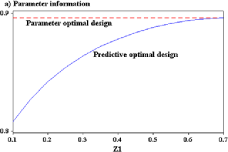
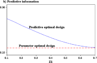
Figure 2: Parameter information per dimension $M(\mathbf{Y};\bolds{\Theta}|Z,\eta)/p$ and predictive information $M(\mathbf{Y};Y_{\nu}|Z,\mathbf{z},\eta)$ under the predictive and parameter optimal designs against $z_{\nu 1},\mathbf{z}_{\nu}^{\prime}\mathbf{z}_{\nu}=1$ for $p=2,n=10,\eta=1,v_{01}=v_{02}=1$.

Example 1.

Let $p=2,n=10,v_{01}=v_{02}=1,\eta=1$ and $\mathbf{z}_{\nu}^{\prime}\mathbf{z}_{\nu}=1$. Figure 2(a) shows the plots of the parameter information measures under the parameter and predictive optimal designs against $z_{\nu 1}$. In order to make the two information measures dimensionally comparable, we have plotted information per parameter $\bar{M}(\mathbf{Y};\Theta|n_{i}^{*})=M(\mathbf{Y};\Theta|n_{i}^{*})/p$. Figure 2(b) shows the plots of the predictive information measures under the parameter and predictive optimal designs. Note that the vertical axes of the two panels are different. These plots show that the parameter (joint) information per dimension is much higher than the predictive information even when the design is optimal for prediction and not for the parameter. The dashed lines show the information quantities for the D-optimal design, which is optimal for the parameter (joint) and for prediction at the diagonal $z_{1}=z_{2}=1/\sqrt{2}\approx 0.707$. The sample is least informative for prediction in this direction. We note that the loss of information for prediction is not nearly as severe as the loss of information about the parameter. This is due to the fact that by Theorem 1, the parameter information measures the joint information about the parameter and prediction and is inclusive of the predictive information. Thus, use of the D-optimal design would be preferable if the experimenter has interest in inference about the parameter as well as about a prediction.

3.2 Optimal Prior Variance

Next we illustrate application to developing prior in the context of a Bayesian solution to the collinearity problem. When the regression matrix $X$ is ill-conditioned, posterior inference about individual parameters is unreliable. The effects of collinearity on the posterior distribution and compensating for the collinearity effects by using $V_{0}=I_{p}$ were discussed by Soofi (1990). In the orthogonal prior variance case $\sum_{j=1}^{p}v_{0j}=p$ is distributed uniformly among the components of $V_{0}$. The following proposition gives an optimal prior variance allocation according to the parameter (joint) information $M(\mathbf{Y};\bolds{\Theta})$ that will be useful when $X^{\prime}X$ is nearly singular.

Proposition 2

Let $\lambda_{1}\geq\cdots\geq\lambda_{p},\sum_{j=1}^{p}\lambda_{j}=p$, and given $\eta$ and $\sum_{j=1}^{p}v_{0j}=c$. The optimal prior variance allocation according to the parameter (joint) information $M(\mathbf{Y};\bolds{\Theta})$ is

$$\cases{v_{01}^{*}=\dfrac{c}{p}+\dfrac{\eta}{p}\displaystyle\sum_{j=2}^{p}(\lambda_{j}^{-1}-\lambda_{1}^{-1}),\cr v_{0j}^{*}=v_{01}^{*}-\eta(\lambda_{j}^{-1}-\lambda_{1}^{-1}),\quad j=2,\ldots,p,}$$ (15)

and the minimum prior variance is determined by $v_{01}^{*}>(\lambda_{p}^{-1}-\lambda_{1}^{-1})\eta$.

See the Appendix.

The optimal information prior (15) allocates prior variances to the components $\theta_{j},j=1,\ldots,p$, based on the eigenvalues $\lambda_{1}\geq\cdots\geq\lambda_{p}$ of $X^{\prime}X$. So it is in the same spirit as Zellner’s $g$ prior (Zellner, 1986) where $v_{0j}\propto\lambda_{j}^{-1},j=1,\ldots,p$. In the same spirit, West (2003) and Maruyama and George (2010) have defined generalized $g$ priors that are applicable when $X$ is singular. Our information optimal allocation scheme is another generalization of the $g$ prior tailored for the collinearity problem where $X$ is full-rank, but nearly singular.

The optimal allocation scheme (15) can be represented in terms of the condition indices $\kappa_{j}=\sqrt{\lambda_{1}/\lambda_{j}}$, $j=1,\ldots,p$, of $X^{\prime}X$ as

$$\cases{\dfrac{\lambda_{1}v^{*}_{01}+\eta}{\lambda_{j}v^{*}_{0j}+\eta}=\kappa^{2}_{j},&$j=2,\ldots,p$,\cr\displaystyle\sum_{j=1}^{p}v^{*}_{0j}=c.}$$

The smallest portion of the total prior variance $v^{*}_{0p}$ is allocated to the component $\theta_{p}$ that corresponds to the smallest eigenvalue $\lambda_{p}$ such that $\frac{\lambda_{1}v^{*}_{01}+\eta}{\lambda_{p}v^{*}_{0p}+\eta}=\kappa^{2}$, where $\kappa=\kappa(X^{\prime}X)=\sqrt{\lambda_{1}/\lambda_{p}}$ is the condition number of $X^{\prime}X$ which is used for collinearity diagnostics (Stewart, 1987; Soofi, 1990; Belsley, 1991).

In some prediction problems, the prediction point $\mathbf{z}_{\nu}$ is given. For example, in the accelerated life testing, $\mathbf{z}_{\nu}$ is the environmental condition and the experiment must be designed such that prediction at $\mathbf{z}_{\nu}$ is optimal. The information decomposition (3) provides the clue when the quantity of interest is the mean response $Q=E(Y|\mathbf{z}_{\nu})$. The components of $\bolds{\theta}=(\theta_{1},\ldots,\theta_{p})^{\prime}$ are independent, a priori and a posteriori, and from (3), $M(\theta_{j},\mathbf{Y}|Z,\eta,V_{0})=0.5\log(1+\eta^{-1}v_{0j}\lambda_{j})$. Under the orthogonal prior, the sample is most informative about the linear combination of the regression coefficients $\theta_{1}=\mathbf{g}_{1}^{\prime}\bolds{\beta}$ where $g_{1}$ is the first eigenvector of $X^{\prime}X$. Thus the optimal design for the expected response at a covariate vector $\mathbf{z}_{\nu}$ is $X^{*}$ such that $\mathbf{z}_{\nu}$ is the first eigenvector of $I_{p}+\eta^{-1}V_{0}X^{*\prime}X^{*}$. Under the uncorrelated prior or weak prior, $X^{*}$ is frequentist E-optimal design, which can be different than the designs that are optimal with respect to parameter (joint) information. The optimal allocation scheme (15) provides improvement to the orthogonal prior for prediction of the expected response when $\mathbf{z}_{\nu}$ is in the space of the eigenvectors corresponding to the large eigenvalues.

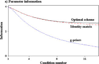
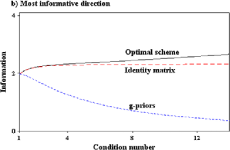
Figure 3: Parameter information $M(\mathbf{Y};\bolds{\Theta}|Z,\eta)$ and information for the most informative direction for prediction of the expected response $M(\mathbf{Y};\theta_{1}|Z,\eta)$ for three types of prior variance allocations ($p=2,c=100,\eta=1$).

Example 2.

Let $p=2,c=100$ and $\eta=1$. Figure 3 compares information measures for the optimal scheme, the orthogonal prior and $V_{0}\propto\Lambda^{-1}$ which is used in some priors such as the $g$-prior.Figure 3(a) shows the plots of parameter information $M(\mathbf{Y};\bolds{\Theta}|Z,\eta)$ against the condition number $\kappa=\sqrt{\lambda_{1}/\lambda_{2}}$ of $X^{\prime}X$. Under all three priors, the parameter information $M(\mathbf{Y};\bolds{\Theta}|Z,\eta)$ decreases with $\kappa$, that is, as the regression matrix descends toward singularity. The parameter information under the optimal scheme slightly dominates the measure under the orthogonal prior, and both dominate the information under the $g$-prior which deteriorates quickly with collinearity. By Theorem 1, the parameter information measure is the joint information about the parameter and prediction and is inclusive of the predictive information. Figure 3(b) shows $M(\mathbf{Y};\theta_{1}|Z,\eta)$ for the direction of the first eigenvector $\theta_{1}=G_{1}^{\prime}\bolds{\beta}$, that is, the most informative direction for prediction of the expected response. The optimal and orthogonal priors improve the information under collinearity, but the measure for the $g$-prior deteriorates quickly.

4 Exponential Family

Consider distributions in the exponential family that provide likelihood functions in the form of

$$\mathcal{L}(\theta)\propto\theta^{n}e^{-\theta s_{n}},\quad\theta>0,$$ (16)

where $s_{n}$ is a sufficient statistic for $\theta$. This is the likelihood function for an important class of models referred to as the time-transformed exponential (TTE) (Barlow and Hsiung, 1983). The TTE models are usually defined in terms of the survival function $\bar{F}(y|\theta)=\exp\{-\theta\phi(y)\},y\geq 0$, where $\phi(y)=-\log\bar{F}_{0}$ and $\theta$ is the “proportional hazard.” The density functions of the TTE models are in the form of

$$f(\phi(y)|\theta)=\theta\phi^{\prime}(y)e^{-\theta\phi(y)},$$ (17)

where $\phi(y)$ is a one-to-one transformation of $Y$ with the exponential distribution $f(y|\theta)=\theta e^{-\theta y}$. For TTE models $s_{n}=\sum_{i=1}^{n}\phi(y_{i})$. Examples include the exponential $\phi(y)=y,y\geq 0$, Weibull $\phi(y)=y^{q},y\geq 0$, Pareto Type I $\phi(y)=\log(y/a),y\geq a>0$, Pareto Type II $\phi(y)=\log(1+y),y\geq 0$, Pareto Type VI $\phi(y)=\log(1+y^{a}),y\geq 0,a>0$ and the extreme value $\phi(y)=e^{y}$.

The family of conjugate priors for (16) is gamma $\mathcal{G}(\alpha,\beta)$ with density function

$$f(\theta)=\frac{\beta^{\alpha}}{\Gamma(\alpha)}\theta^{\alpha-1}e^{-\beta\theta}.$$ (18)

The posterior distribution is $\mathcal{G}(\alpha+n,\beta+s_{n})$.

The information in the observed sample is given by

$$\Delta H(\mathbf{y};\Theta)=H_{\mathcal{G}}(\alpha)-H_{\mathcal{G}}(\alpha+n)+\log\biggl{(}1+\frac{s_{n}}{\beta}\biggr{)},$$

where $H_{\mathcal{G}}(\alpha)$ is the entropy of $\mathcal{G}(\alpha,1)$ given by

$$H_{\mathcal{G}}(\alpha)=\log\Gamma(\alpha)-(\alpha-1)\psi(\alpha)+\alpha,$$

and $\psi(\alpha)=\frac{d\log\Gamma(\alpha)}{d\alpha}$ is the digamma function.

For the TTE family (17), the marginal distribution of $s_{n}$ is inverted beta (beta prime) distribution with density

$$f(s_{n})=\frac{1/\beta}{B(\alpha,n)}\frac{(s_{n}/\beta)^{n-1}}{(1+s_{n}/\beta)^{\alpha+n}},\quad s_{n}\geq 0,$$

where $B(\alpha,n)$ is the beta function. Using $E_{s_{n}}\{\log(1+\frac{s_{n}}{\beta})\}=\psi(\alpha+n)-\psi(\alpha)$, the expected information for all models with likelihood functions in the form of (16) is

$$M[\mathbf{Y};(\Theta;Y_{\nu})] = M(\mathbf{Y};\Theta)$$

$$= H_{\mathcal{G}}(\alpha)-H_{\mathcal{G}}(\alpha+n)$$

$${}+\psi(\alpha+n)-\psi(\alpha).$$

An interesting property of (4) is the following recursion:

$$M(\mathbf{Y}_{n};\Theta|\alpha) = M(\mathbf{Y}_{n-1};\Theta|\alpha)$$

$${}+K_{\mathcal{G}}(\alpha+n-1),$$

where $\mathbf{Y}_{n}$ and $\mathbf{Y}_{n-1}$ are vectors of dimensions $n$ and $n-1$, and

$$K_{\mathcal{G}}(v)=K(\mathcal{G}_{v}\dvtx\mathcal{G}_{v+1})=\frac{1}{v}+\psi(v)-\log v$$ (21)

is the Kullback–Leibler information between $\mathcal{G}_{v}=\mathcal{G}(\nu,\beta)$ and $\mathcal{G}_{v+1}=\mathcal{G}(\nu+1,\beta)$. The recursion (4) is found using $\psi(\alpha+1)=\psi(\alpha)+\frac{1}{\alpha}$. By (4), $M(\mathbf{Y}_{n};\Theta|\break\mathbf{Y}_{n-1})=K_{\mathcal{G}}(\alpha+n-1)$. That is, on average, the incremental contribution of an additional observation is equivalent to the information divergence due to one unit increase of the prior shape parameter.

The prior predictive distribution for the exponential model is Pareto $\mathcal{P}(\alpha,\beta)$ with density function

$$f(y_{\nu})=\frac{\alpha\beta^{\alpha}}{(\beta+y_{\nu})^{\alpha+1}},\quad y_{\nu}\geq 0.$$

The posterior predictive distribution $f(y_{\nu}|\mathbf{y})$ is also Pareto with the updated parameters $\mathcal{P}(\alpha+n,\beta+s_{n})$. The predictive information measures are given by

$$\Delta H(\mathbf{y};Y_{\nu}) = H_{\mathcal{P}}(\alpha)-H_{\mathcal{P}}(\alpha+n)$$

$${}-\log\biggl{(}1+\frac{s_{n}}{\beta}\biggr{)},$$

$$M(\mathbf{Y};Y_{\nu}) = H_{\mathcal{P}}(\alpha)-H_{\mathcal{P}}(\alpha+n)$$

$${}-\psi(\alpha+n)+\psi(\alpha),$$

where $H_{\mathcal{P}}(\alpha)=\frac{1}{\alpha}-\log\alpha+1$ is the entropy of $\mathcal{P}(\alpha,1)$.

By invariance of the mutual information, the expected predictive information for TTE family (17) is given by (4).

By Theorem 1, $\Delta H[s_{n};(\Theta,Y_{\nu})]=\Delta H(\mathbf{y};\Theta)$,$M[\mathbf{Y};(\Theta,Y_{\nu})]=M(\mathbf{Y};\Theta)$ and $M(\mathbf{Y};Y_{\nu})\leq M(\mathbf{Y};\break\Theta)$. The following theorem gives a more specific pattern of relationships.

Theorem 2

The following results hold for the TTE family (17) and gamma prior (18): [(a)]

$M(\mathbf{Y};\Theta|\alpha)$ and $M(\mathbf{Y};Y_{\nu}|\alpha)$ are decreasing functions of $\alpha$, increasing functions of $n$ and as $n\to\infty$, $M(\mathbf{Y}_{n+1};\Theta|\alpha)-M(\mathbf{Y}_{n};\Theta|\alpha)\to 0$ and $M(\mathbf{Y};Y_{\nu}|\alpha)\to K_{\mathcal{G}}(\alpha)$.

$M(\mathbf{Y};\Theta|\alpha)=M(\mathbf{Y};Y_{\nu}|\alpha)+M(\mathbf{Y};\Theta|\alpha+1)$, where $M(\mathbf{Y};\Theta|\alpha+1)$ is the sample information with gamma prior $\mathcal{G}(\alpha+1,\beta)$.

$M(\mathbf{Y};\Theta|\alpha)-M(\mathbf{Y};Y_{\nu}|\alpha)$ increases with $\alpha$ and with $n$.

For (a), it is known that the expected parameter and predictive measures are increasing functions of $n$. It was shown by Ebrahimi and Soofi (1990) that for the exponential model, $M(\mathbf{Y};\Theta|\alpha)$ is decreasing in $\alpha$. By the invariance of the mutual information the same result holds for the TTE family. The limits are found by noting that $K_{\mathcal{G}}(v)\to 0$ as $v\to\infty$. The expected predictive measure decreasing in $\alpha$ is found by taking the derivative, using series expansion of the trigamma function $\psi^{\prime}(u)=\sum_{k=1}^{\infty}\frac{1}{(u+k)^{2}}$ (Abramowitz and Stegun, 1970), and an induction on $n$ that shows the derivative is negative. Part (b) is found using recursion $\psi(\alpha+1)=\psi(\alpha)+\frac{1}{\alpha}$. Part (c) is implied by (a) and (b). The difference is $M(\mathbf{Y};\Theta|\alpha+1)$ which is increasing (decreasing) in $n$ ($\alpha$).

By part (a) of Theorem 2, the parameter and predictive information both increase with $n$. Part (b) of Theorem 2 gives the relationship between the parameter (joint) and the predictive information measures. Part (c) indicates that under conditional independence, the parameter (joint) information grows faster than the predictive information with the sample size.

Example 3.

As an application, consider Type II censoring where observing the number of failures is a design parameter. For the exponential model, the sufficient statistic for $\theta$ in (16) is the total time under the test

$$t_{r}=y_{1}+\cdots+y_{r-1}+(n-r+1)y_{r},\quad r\leq n,$$

where $y_{1}\leq y_{2}\leq\cdots\leq y_{n}$ are the order statistics of a sample of size $n$. The parameter information $M(T_{r};\break\Theta|n)$ is given by (4) and the predictive information $M(T_{r};Y_{\nu}|\alpha,n)$ is given by (4) with $n=r$. Ebrahimi and Soofi (1990) examined the loss of information about the exponential failure rate. By part (a) of Theorem 2, censoring also results in loss of predictive information. As in the case of parameter information, the loss of predictive information can be compensated by the prior parameter $\alpha$. Figure 4 shows plots of the expected parameter and predictive information measures. Figure 4(a) illustrates the information decomposition part [Theorem 2, part (b)] for $\alpha=1$ as function of $n$. The parameter information and predictive information are both increasing in $n$. The parameter information increases at a faster rate than the predictive information. In this case, the difference between the parameter and predictive information is $M(\mathbf{y};\Theta|\alpha+1)$, also shown in Figure 4(a). These information measures are decreasing in $\alpha$. Figure 4(b) shows the plots of loss of information due to Type II censoring for $n=25$ and $\alpha=1,2$. We note that the predictive information loss is not as severe as the parameter information loss. As seen in the figure, the information losses can be recovered by increase in prior precision.

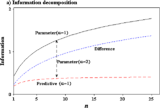
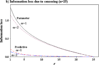
Figure 4: Decomposition of the joint (parameter) information $M(T_{r};\Theta|\alpha,n)$ into predictive information $M(T_{r};Y_{\nu}|\alpha,n)$ and $M(T_{r};\Theta|\alpha+1,n)$ and loss of information $M(T_{n};\Theta|\alpha)-M(T_{r};\Theta|\alpha)$ due to Type II censoring of exponential data.

By part (a) of Theorem 2, $M(\mathbf{Y};\Theta)$ and $M(\mathbf{Y};Y_{\nu})$ are maximized by choosing $\alpha$ as small as possible. It is natural to expect that the limiting case, which is the Jeffreys prior $f(\theta)\propto\theta^{-1}$, be optimal with respect to both the parameter and prediction information. But its use is consequential. Since the Jeffreys prior is improper, the expected parameter information is given by the negative conditional entropy of the posterior distribution, which is proper. However, unlike the mutual information, the entropy is not invariant under one-to-one transformations and the result depends on the parametric function of interest. For example, for the exponential model, the posterior distribution of failure rate $\theta$ is gamma $f(\theta|s_{n})=\mathcal{G}(n,s_{n})$ and its entropy is $H[f(\theta|s_{n})]=H_{\mathcal{G}}(n)-\log s_{n}$. The distribution of $S_{n}$ is Pareto$f(s_{n})\propto s_{n}^{-n}$ which is proper for $n>1$ and $s_{n}\geq s_{0}>0$. The expected parameter information, $\mathcal{I}(\Theta|S_{n})=-\mathcal{H}[f(\theta|s_{n})]$, is a decreasing function of $n$. But the posterior distribution of the mean parameter $\mu=\theta^{-1}$ is inverse-gamma and information about the mean is increasing in $n$. With the Jeffreys prior, the prior predictive distribution is also improper. The posterior predictive is Pareto $\mathcal{P}(n,s_{n})$ and its entropy is $H[f(Y_{\nu}|s_{n})]=H_{\mathcal{P}}(n)+\log s_{n}$. The expected predictive information is $\mathcal{I}(Y_{\nu}|S_{n})=-\mathcal{H}[f(Y_{\nu}|s_{n})]$, which is an increasing function of $n$.

5 Dependent Sequences

When the sequence of random variables $Y_{i}|\theta,i=1,2,\ldots,$ is not conditionally independent, the information provided by the sample about the parameter and prediction jointly decomposes as

$$\quad M[\mathbf{Y};(\Theta,Y_{\nu})] = M(\mathbf{Y};\Theta)+M(\mathbf{Y};Y_{\nu}|\Theta)$$

$$= M(\mathbf{Y};Y_{\nu})+M(\mathbf{Y};\Theta|Y_{\nu}),\vspace*{-2pt}$$

where $M(\mathbf{Y},Y_{\nu}|\Theta)\geq 0$ is the measure of conditional dependence, hence the inequality becomes equality for the case of conditional independence and (5) gives (9). Thus, for the conditionally dependent sequence, $M[\mathbf{Y};(\Theta,Y_{\nu})]$ exceeds $M(\mathbf{Y};\Theta)$ by theamount $M(\mathbf{Y};Y_{\nu}|\Theta)>0$. Also from (5), we find that

$$M(\mathbf{Y};\Theta) \leq M(\mathbf{Y};Y_{\nu})\quad\mbox{if and only if}$$

$$M(\mathbf{Y};\Theta|\mathbf{y}_{\nu}) \leq M(\mathbf{Y};Y_{\nu}|\Theta).\vspace*{-2pt}$$

For strongly conditional dependent sequence, the second inequality is plausible and the predictive information $M(\mathbf{Y},Y_{\nu})$ can dominate the parameter information $M(\mathbf{Y};\Theta)$.

=370pt Uncorrelated (UC) Intraclass (IC) Serial correlation (SC) Conditional sequence    $|R|\theta|$ 1 $[1+(n-1)\rho](1-\rho)^{n-1}$ $1-\rho^{2}$    $T_{n}(R|\theta)$ $n$ $\frac{n}{1+(n-1)\rho}$ $\frac{n-(n-2)\rho}{1+\rho}$    $\rho^{2}_{y_{\nu},\mathbf{y}|\theta}$ 0 $\frac{n\rho^{2}}{1+(n-1)\rho}$ $\rho^{2}$ Predictive sequence    $\rho^{2}_{p}$ $\frac{1}{1+\eta}$ $\frac{1+\eta\rho}{1+\eta}$ $\frac{1+\eta\rho^{k}}{1+\eta}$    $\rho^{2}_{y_{\nu},\mathbf{y}}$ $\frac{n}{(1+\eta)(n+\eta)}$ $\frac{n\rho^{2}_{p}}{1+(n-1)\rho_{p}}$ Immediate future $\rho^{2}_{p}$

Table 1: Formulas for uncorrelated, intraclass and serial correlation models

In this section we first examine the effects of correlation between observations on the information about the mean parameter and prediction where the data are normally distributed. We then consider order statistics where no particular prior distribution and model for the likelihood function are assumed.

5.1 Intraclass and Serially Correlated Models

We consider the intercept linear model $f(\mathbf{y}|\theta)=N(\theta\mathbf{z},\sigma_{1}^{2}R)$, where $\mathbf{z}$ is an $n\times 1$ vector of ones and $R=R|\theta=[\rho_{ij|\theta}]$ is a known correlation matrix. By invariance of the mutual information, the results hold for all distributions of variables that are one-to-one transformations of elements of $\mathbf{y}$, for example, log-normal model. As before, $\sigma_{1}^{2}>0$ is known and $f(\theta)=N(\mu_{0},\sigma_{0}^{2})$. The posterior variance is given by $\sigma^{2}_{\theta|\mathbf{y}}=\sigma_{0}^{2}[1+T_{n}(R)\eta^{-1}]^{-1}$, where $T_{n}(R)=\mathbf{z}^{\prime}R^{-1}\mathbf{z}$ is the sum of all elements of $R^{-1}$. The parameter information is given by

$$M(\mathbf{Y};\Theta|R)=0.5\log\bigl{(}1+\eta^{-1}T_{n}(R)\bigr{)}.\vspace*{-2pt}$$ (24)

The following representations facilitate computation and study of the predictive and joint information measures. If $Y_{\nu}$ and $Y_{\nu}|\mathbf{y}$ are normal, then the predictive information is given by

$$M(\mathbf{Y};Y_{\nu}) = -0.5\log(1-\rho^{2}_{y_{\nu},\mathbf{y}})$$

$$= 0.5\log[C^{-1}]_{\nu\nu},$$

where $\rho^{2}_{y_{\nu},\mathbf{y}}$ is the square of unconditional multiple correlation coefficient of the regression of $Y_{\nu}$ on $\mathbf{y}$, $C=[c_{ij}],i,j=1,\ldots,n+1$, denotes the correlation matrix of the $(n+1)$-dimensional vector $(\mathbf{Y},Y_{\nu})$, and $[C^{-1}]_{\nu\nu}$ denotes the $(\nu,\nu)$ element of $C^{-1}$.

The joint information about the parameter and prediction can be computed by the first decomposition in (5),

$$\qquad M[\mathbf{Y};(\Theta,Y_{\nu})]=M(\mathbf{Y};\Theta|R)+M(\mathbf{Y},Y_{\nu}|\Theta),$$ (26)

where $M(\mathbf{Y};\Theta|R)$ is given in (24) and the measure of conditional dependence can be computed similarly to (5.1):

$$M(\mathbf{Y};Y_{\nu}|\Theta) = -0.5\log(1-\rho^{2}_{y_{\nu},\mathbf{y}|\theta})$$

$$= 0.5\log[C^{-1}|\theta]_{\nu\nu}\geq 0,$$

where $\rho^{2}_{y_{\nu},\mathbf{y}|\theta}$ is the square of conditional multiple correlation coefficient and $C|\theta=[c_{ij}|\theta],i,j=1,\ldots,\break n+1$, is the correlation matrix of conditional distribution of $(\mathbf{Y},Y_{\nu})$, given $\theta$. Note that $C|\theta$ includes $R$ and an additional row and column for $Y_{\nu}$.

Measures such as the determinant $|R|$ and condition number $\kappa(R)=\sqrt{\lambda_{1}/\lambda_{n}}$, where $\lambda_{1}<\cdots<\lambda_{n}$ are eigenvalues of $R$, can be used to rank dependence of the normal samples. However, in general, these measures do not provide a unique ranking. In order to rank the dependence uniquely as well as for ranking the predictive information in terms of sample dependence, we assume some structures for $R$. We consider two important models: the intraclass (IC) model with $\rho_{ij|\theta}=\rho$ for all $i\neq j$, and the serial correlation (SC) model with $\rho_{i,i\pm k|\theta}=\rho^{k}\geq 0,k>0$. Dependence within each of these models and between the two models is ranked uniquely by $|R|$ and $\kappa(R)$.

Table 1 shows $|R|$ and $T_{n}(R)$ for the IC, SC models along with the independent (uncorrelated) model (UC). The determinants and inverses of the IC and SC matrices are well known. Using $T_{n}(R)$ in (24) gives the parameter information. The third row of Table 1 shows $\rho^{2}_{y_{\nu},\mathbf{y}|\theta}$ which is computed using (5.1) with $(n+1)$-dimensional IC and SC structures for $C$. Table 1 also shows the square of unconditional (predictive) correlation $\rho^{2}_{p}=c_{ij}$, which is used in (5.1) for computing the predictive information measures. Computation of $\rho^{2}_{p}=c_{ij}$ is shown in the Appendix. The last row of Table 1 shows the square of unconditional multiple correlation coefficient $\rho^{2}_{y_{\nu},\mathbf{y}}$ computed from (5.1). The predictive measure for the SC model is for the one-step prediction.

The effects of prior on the information quantities are induced through $\eta$ which is proportional to prior precision. Clearly (24) is decreasing in $\eta$. Using the last two rows of Table 1 it can be shown that (5.1) and the difference between (24) and (5.1) are also decreasing in $\eta$. Thus, the optimal prior for inference about the parameter and prediction is to choose the prior variance as large as possible.

The following theorem summarizes the effects of the IC and SC correlation structures on the normal information measures (24)–(26).

Theorem 3

[(a)]

For all three models, $M(\mathbf{Y};\Theta|\rho)$, $M(\mathbf{Y};Y_{\nu}|\rho)$ and $M[\mathbf{Y};(\Theta,Y_{\nu})|\rho)]$ increase with $n$ and decrease with $\eta$.

For both IC and SC models, $M(\mathbf{Y};\Theta|\rho)$ decreases with $\rho$, and

$$M^{\mathit{IC}}(\mathbf{Y};\Theta|\rho)\leq M^{\mathit{SC}}(\mathbf{Y};\Theta|\rho)\leq M^{\mathit{UC}}(\mathbf{Y};\Theta),$$

where the last equality holds if and only if $\rho=0$.

For both IC and SC models, $M(\mathbf{Y};Y_{\nu}|\rho)$ increases with $\rho$, and

$$M^{\mathit{IC}}(\mathbf{Y};Y_{\nu}|\rho)\geq M^{\mathit{SC}}(\mathbf{Y};Y_{\nu}|\rho)\geq M^{\mathit{UC}}(\mathbf{Y};Y_{\nu}),$$

where the last equality holds if and only if $\rho=0$.

For both IC and SC models, $M[\mathbf{Y};(\Theta,Y_{\nu})|\rho)]$ decreases in $\rho$ for $\rho\leq\rho_{0}(n,\eta)$ and increases in $\rho$ for $\rho>\rho_{0}(n,\eta)$, where $\rho_{0}^{\mathit{IC}}(n,\eta)$ and $\rho_{0}^{\mathit{SC}}(n,\eta)$ are roots of quadratic equations and both are increasing in $n$ and decreasing in $\eta$.

(a) Can be easily seen by taking derivatives. (b) It is also easy to see that for the correlated models $T_{n}(R)$ are decreasing functions of $\rho$ and that $T^{\mathit{IC}}_{n}(R)\leq T^{\mathit{SC}}_{n}(R)\leq T^{\mathit{UC}}_{n}(R)=n$. (c) This is implied by the facts that $\rho^{\mathit{IC}}_{p}>\rho^{\mathit{SC}}_{p}$ and the predictive information increases with $\rho$, as expected. (d) Taking the derivative, $\rho_{0}(n,\eta)$ is given by the root of $A_{n,\eta}\rho^{2}+B_{n,\eta}\rho+C_{n,\eta}=0$, where $A_{n,\eta}^{\mathit{IC}}=n-1,B_{n,\eta}^{\mathit{IC}}=2(1+n\eta^{-1}),A_{n,\eta}^{\mathit{SC}}=1+(2n-1)\eta^{-1},B_{n,\eta}^{\mathit{SC}}=1+(2n-1)\eta^{-1}$ and $C_{n,\eta}=(1-n)\eta^{-1}$. For each model there is only a unique positive solution.

Theorem 3 formalizes the intuition that samples with stronger dependence are less informative about the parameter and more informative about prediction. Since $M(\mathbf{Y};\Theta|\rho)$ is increasing in $n$, one can compensate the loss of parameter information due to the dependence by increasing the sample size. The following example illustrates these and some other noteworthy points.

Example 4.

[(a)]

Figure 5 shows plots of $M(\mathbf{Y};\Theta|\rho)$ and $M(\mathbf{Y};\break Y_{\nu}|\rho)$ against sample size for the UC model and the correlated models IC and SC with $\rho=0.50,0.75$. Plots in panels (a) and (b) reveal the following features. [(iii)]

All information measures are increasing in $n$.

For the UC model, the parameter information is the highest and has the fastest rate of increase with $n$, and the predictive information is the lowest with the slowest (almost flat) rate of increase.

For the SC model, the parameter information is higher and increases much faster than the predictive information.

For the IC model, the parameter information is lower than the predictive information while both measures have about the same rates of increase.

Interestingly, for the UC and SC models, the differences between the parameter and predictive information measures grow with $n$ much faster than the predictive information measures. That is, the share of predictive information decreases with the sample size.

As can be seen in Figure 5(a), to gain about one unit (nit) of information, we need $n=3$ from the UC, and with $\rho=0.50,0.75$, we need $n=8,16$ observations under SC, and $n=26,37$ observations under IC models, respectively.

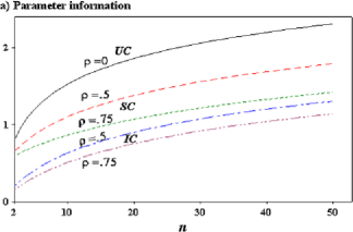
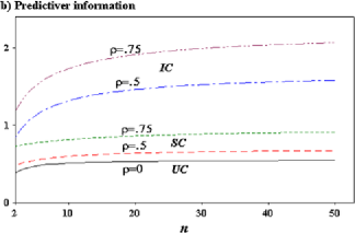
Figure 5: The parameter information $M(\mathbf{Y};\Theta|\rho)$ and predictive information $M(\mathbf{Y};Y_{\nu}|\rho)$ for the independent, IC and SC normal models as functions of the sample size ($\eta=0.5$).

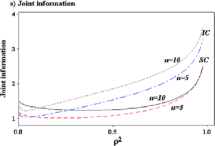
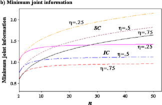
Figure 6: The joint parameter and predictive information $M[\mathbf{Y};(\Theta,Y_{\nu})|\rho]$ and minima of the joint information $\min_{\rho}M[\mathbf{Y};(\Theta,Y_{\nu})|\rho]$ for SC and IC normal models.

Figure 6(a) shows the plots of the joint information measures for the SC and IC models as functions of $\rho^{2}$ for $n=5,10$ and $\eta=0.5$. Note that the joint information of the SC model dominates the joint information of the IC model when dependence is weak. After the minimum point, the rate of growth of joint information for the IC model is steep and the IC information measure dominates the SC information measure when the dependence is rather strong.

Figure 6(b) shows the plots of the minimum joint information measures for the SC and IC families as functions of $n$ for $\eta=0.25,0.5,0.75$. These plots are useful for determining sample size for each family such that the minimum information exceeds a given value. For example, to gain about 1.5 units (nits) of information from an SC sample with unknown $\rho$, we need $n=9,25,37$ with $\eta=0.25,0.50,0.75$, respectively. The plots show that

$$M^{\mathit{IC}}_{0}[\mathbf{Y};(\Theta,Y_{\nu})|n,\eta]\leq M^{\mathit{SC}}_{0}[\mathbf{Y};(\Theta,Y_{\nu})|n,\eta],$$

where $M_{0}[\mathbf{Y};(\Theta,Y_{\nu})|n,\eta]=\min_{\rho}M[\mathbf{Y};(\Theta,Y_{\nu})|\rho]$.This inequality can be proved by substituting$\rho_{0}^{\mathit{IC}}(n,\eta)$ and $\rho_{0}^{\mathit{SC}}(n,\eta)$ in the expressions for $T_{n}(R)$ and $\rho^{2}_{y_{\nu},\mathbf{y}|\theta}$.

5.2 Order Statistics

Let $Y_{1}\leq Y_{2}\leq\cdots\leq Y_{n}$ be the order statistics of conditionally independent sample $X_{1},\ldots,X_{n}$ from a continuous distribution with density function $g(x|\theta)$, and let $\mathbf{y}_{r}=(y_{1},\ldots,y_{r}),r\leq n$. Conditional on $\theta$, the order statistics have a Markovian dependence structure (Arnold, 1992). The mutual information between consecutive order statistics is given by

$$M(Y_{r};Y_{r+1}|\theta)$$

$$\quad=M_{n}(r)$$

$$\quad=\log B(r+1,n-r+1)+\log(n+1)-1$$ (28)

$$\qquad{}-r\{\psi(r)-\psi(n)\}$$

$${}\qquad-(n-r)\{\psi(n-r)-\psi(n)\};$$

see the article by Ebrahimi, Soofi and Zahedi (2004). That is, $M_{n}(r)$ is the measure of Markovian dependence between order statistics of the independent sample conditional on $\theta$. It was shown by Ebrahimi, Soofi and Zahedi (2004) that $M_{n}(r)$ is increasing in $n$, and for a given $n$, the information is symmetric in $r$ and $n-r$, and attains its maximum at the median (see Figure 7). The next lemma gives generalizations of (5.2). All information functions are conditional on $r$ and $n$, which will be suppressed when unnecessary.

Lemma 1.

Let $Y_{1}\leq\cdots\leq Y_{n}$ denote the order statistics of random variables $X_{1},\ldots,X_{n}$ which, given $\theta$, are independent and have identical distribution $g(x|\theta)$ and $\mathbf{Y}_{r}$ and $\mathbf{Y}_{q}$ denote the disjoint subvectors of order statistics. Then:

$M(\mathbf{Y}_{r};\mathbf{Y}_{q}|\theta)$ is free from the parent distribution $g(x|\theta)$ and the prior distribution $f(\theta)$.

For any two consecutive subvectors $\mathbf{Y}_{r}=\break(Y_{k+1},\ldots,Y_{k+r})$ and $\mathbf{Y}_{q}=(Y_{k+r+1},\ldots,Y_{k+r+q})$,$M(\mathbf{Y}_{r};\mathbf{Y}_{q}|\theta)=M_{n}(k+r)$.

Let $U=G(X)$. Then $U$ is uniform and its order statistics $W_{1}\leq W_{2}\leq\cdots\leq W_{n}$ are given by $W_{i}=G(Y_{i})$, and $\mathbf{W}_{r}$ and $\mathbf{W}_{q}$ are the subvectors corresponding to $\mathbf{Y}_{r}$ and $\mathbf{Y}_{q}$. Since $W_{i}=G(Y_{i})$ is one-to-one, we have $M(\mathbf{Y}_{r};\mathbf{Y}_{q})=M(\mathbf{W}_{r};\mathbf{W}_{q})$. Furthermore the distribution of any subset of order statistics is ordered Dirichlet with parameters $n$ and the indices of the order statistics contained in the subset, hence $M(\mathbf{Y}_{r};\mathbf{Y}_{q})=M(\mathbf{W}_{r};\mathbf{W}_{q})$ is free from the parent distribution $g(x|\theta)$. Part (b) follows from $Y_{1}|\theta,\ldots,Y_{n}|\theta$ being a Markovian sequence.

It can easily be shown that information provided by the first $r$ order statistics about the parameter $M(\mathbf{Y}_{r},\Theta)$ satisfies (4). The predictive distributions of order statistics are given by $f(y_{i})=\int f(y_{i}|\theta)\*f(\theta)\,d\theta$, $i=1,\ldots,n$. Note that $y_{1}\leq y_{2}\leq\cdots\leq y_{n}$ are the order statistics of a sample of the exchangeable sequence $X_{1},\ldots,X_{n}$, unconditionally. The following results provide some insight about the parameter and predictive information for order statistics.

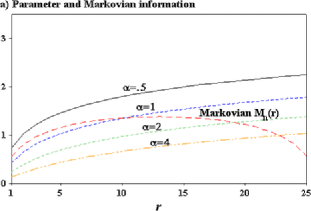
(a)

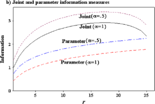
(b)

Figure 7: Expected information about the parameter $M(\mathbf{Y}_{r},\Theta)$ and the joint information about the parameter and prediction of the $(r+1)$st order statistic $M[\mathbf{Y}_{r};(\Theta,Y_{r+1})]$ provided by the vector of preceding order statistics $\mathbf{Y}_{r}$, and the information due to the Markovian dependence between order statistics ($n=26$).

Theorem 4

Let $M[\mathbf{Y}_{r};(\Theta,Y_{r+1})]$ denote the information provided by the first $r$ order statistics about the parameter and for prediction of the next order statistic jointly. Then:

$M[(\mathbf{Y}_{r};(\Theta,Y_{r+1})]=M(\mathbf{Y}_{r};\Theta)+M_{n}(r)\geq\break M(\mathbf{Y}_{r};\Theta)$.

The following statements are equivalent: [(ii)]

$M(\mathbf{Y}_{r};Y_{r+1})\geq(\leq)M_{n}(r)$.

$M(\Theta;Y_{r+1})\geq(\leq)M(\mathbf{Y}_{r+1};\Theta)-M(\mathbf{Y}_{r};\Theta)$,where $\mathbf{Y}_{r+1}=(Y_{1},\ldots,Y_{r},Y_{r+1})$.

Using the following decompositions of mutual information, we have

$$M[(\Theta,Y_{r+1});\mathbf{Y}_{r}]=M(\mathbf{Y}_{r};\Theta)+M(\mathbf{Y}_{r};Y_{r+1}|\Theta).$$

Applying part (b) of Lemma 1 to the second term gives the result (a). For (b) we use the following decompositions of mutual information:

$$M[(\mathbf{Y}_{r},\Theta);Y_{r+1}] = M(\mathbf{Y}_{r};Y_{r+1})+M(\Theta;Y_{r+1}|\mathbf{Y}_{r})$$

$$= M(\Theta;Y_{r+1})+M(\mathbf{Y}_{r};Y_{r+1}|\Theta).$$

Equating the two decompositions with $M(Y_{r+1};\mathbf{Y}_{r}|\break\Theta)=M_{n}(r)$ gives equivalence of (i) and

$$M(\Theta;Y_{r+1})\geq(\leq)M(\Theta;Y_{r+1}|\mathbf{Y}_{r}).$$ (29)

The equivalence with (ii) is obtained by solving

$$M(\mathbf{Y}_{r+1};\Theta)=M(\mathbf{Y}_{r};\Theta)+M(\Theta;Y_{r+1}|\mathbf{Y}_{r})$$

for $M(\Theta;Y_{r+1}|\mathbf{Y}_{r})$ and substituting in (29).

Part (a) of Theorem 4 shows $M[\mathbf{Y}_{r};(\Theta,Y_{r+1})]$ is inclusive of Lindley’s measure reflecting the fact that conditional on $\theta$, order statistics are dependent. So the information provided by the first $r$ order statistics about the parameter and for prediction of the next order statistic is more than the information provided about the parameter. However, the excess information amount measures the Markovian dependence between order statistics of the independent sample and does not depend on $g_{x|\theta}$ and $f_{\theta}$. An implication of this result is that reference posterior corresponding to the prior that maximizes the parameter information $M(\mathbf{Y}_{r};\Theta)$ also remains optimal with respect to $M[\mathbf{Y}_{r};(\Theta,Y_{r+1})]$.

Part (b) of Theorem 4 gives the equivalence of the orders of information in terms of (i) the predictive and sample order statistics and (ii) the expected information about the parameter provided by an order statistic in terms of the incremental amount of information provided about the parameter.

Example 5.

For the case of exponential model with the gamma prior, the conditional distribution of $(r+1)$st order statistic given $\theta$ and the first $r$ order statistics is exponential with density

$$f(y_{r+1}|y_{r},\theta)$$

(30)

$$\quad=(n-r)\theta e^{-\theta(n-r)(y_{r+1}-y_{r})},\quad y_{r+1}>y_{r}.$$

The posterior predictive distribution of $(r+1)$st order statistic given first $r$ order statistics is Pareto with parameters $\alpha+r,b_{r}=\frac{\beta+t_{r}}{n-r}$ and a location parameter $y_{r}$. Since entropy is location-invariant,$H(Y_{r+1}|\mathbf{y}_{r})$ is $H(Y_{r+1}|t_{r},y_{r},r,n)=H(Y_{\nu}|t_{r},r)-\break\log(n-r)$. Figure 7 illustrates some properties of these information measures for the exponential model and $n=26$. [(a)]

Figure 7(a) shows plots of $M(\mathbf{Y}_{r};\Theta|\alpha,n)=M(T_{r};\Theta|\alpha,n)$ for $\alpha=0.5,1,2,4$, superimposed by the Markovian dependence information measure $M_{n}(r)$ for the order statistics. Since $M(T_{r};\Theta|\alpha,n)$ is increasing in $r$, censoring results in loss of information about the parameter. Thus, without consideration of cost of the experiment, $r^{*}=n=26$. Since $M_{n}(r)$ is decreasing for $r$ larger than the median, censoring beyond the median results in gain of information about the next outcome.

Figure 7(b) shows the plots of the parameter information $M(\mathbf{Y}_{r};\Theta|\alpha,n)$ and joint information $M[\mathbf{Y}_{r};(\Theta,Y_{r+1})|\alpha,r,n]$ computed using part (a) of Theorem 4 for $\alpha=0.5,1$. We note that $M[\mathbf{Y}_{r};(\Theta,\break Y_{r+1})|\alpha,r,n]$ is not monotone because the Markovian dependence information measure $M_{n}(r)$decreases for the order statistics above the median. The optimal $r$ for the joint parameter and predictive information, without consideration of cost the experiment, is $r^{*}=17<n$. Thus, unlike the case of conditionally independent model, the parameter information utility and the joint parameter–predictive information utility lead to different sampling plans.

In Section 4 we noted that under the Jeffreys prior, at least one observation is needed for obtaining a proper posterior. Following this idea more generally, we compare the expected uncertainty change due to the first $r$ order statistics with the first order statistic $r=1$, given by

$$\mathcal{B}[\mathbf{Y}_{r};(\Theta,Y_{r+1})]=H[(\Theta,Y_{1})]-\mathcal{H}[(\Theta,Y_{r+1})|\mathbf{Y}_{r}],$$

where $\mathcal{H}[(\Theta,Y_{r+1})|\mathbf{Y}_{r}]=E_{s_{r}}\{H[(\Theta,Y_{r+1})|\mathbf{Y}_{r}]\}$ is the conditional joint entropy of $(\Theta,Y_{r+1})$ given the first order statistic, averaged with respect to $f(\mathbf{y}_{r})$. The expected uncertainty change $\mathcal{B}(\mathbf{Y}_{r};Y_{r+1})$ for prediction of $(r+1)$st order statistic is defined similarly. These measures, which can be referred to as the information bridge between the first and $(r+1)$st order statistics, are invariant under linear transformations, but can be negative. It can be shown that for any parent distribution $g(x|\theta)$ where $\theta$ is the scale parameter and any prior $f(\theta)$,

$$M(\mathbf{Y}_{r};\Theta) = \mathcal{B}[\mathbf{Y}_{r};(\Theta,Y_{r+1})]+\log\biggl{(}\frac{n}{n-r}\biggr{)},$$

$$M(\mathbf{Y}_{r};Y_{r+1}) = \mathcal{B}(\mathbf{Y}_{r};Y_{r+1})+\log\biggl{(}\frac{n}{n-r}\biggr{)}.$$

Clearly, $\mathcal{B}(\cdot,\cdot|r,n)\to M(\cdot,\cdot|r,n)$ as $\frac{r}{n}\to 0$. So, the quantity $\log(\frac{n}{n-r})$ can be interpreted as the finite sample correction factor for the information.

6 Conclusions

This article is the first attempt to study the relationship between the parameter and predictive information measures, the analytical behavior of the predictive information in terms of prior parameters and the effects of conditional dependence between the observable quantities on the Bayesian information measures. We provided analytical results and showed applications in some statistical and modeling problems.

The measure of information that sample provides about the parameter and prediction jointly led to some new insights about the marginal parameter and predictive information measures. For the case of conditionally independent observations, decompositions of the joint information revealed that the parameter information is in fact the measure of information about the parameter and prediction jointly. This finding implies that all existing results about Lindley’s information are applicable to the joint measure of parameter and predictive information. In particular, the reference posterior and the optimal design that maximize the sample information about the parameter are also optimal solutions for the sample information about the parameter and prediction jointly. Yet another information decomposition revealed that predictive information is a part of the information that sample provides about the parameter.

We examined interplay between the information measures and the prior and design parameters for two general classes of models: the linear models for the normal mean, and a broad subfamily of the exponential family. A few applications showed the usefulness of the information measures and some insights were developed. A proposition provided the optimal designs with respect to the parameter (joint) information and predictive information measures for an ANOVA type model. The results include the minimum sample sizes required in terms of the given prior variances and the covariate vector for the prediction. Another proposition provided the optimal prior variance allocation scheme with respect to the parameter (joint) information for collinear regression, which includes the minimum prior variance required for the problem. Examples for the linear and the exponential family models revealed that the predictive information provided by the conditionally independent sample is only a small fraction of the parameter (joint) information and the gap between the parameter and predictive information measures grows rapidly with the sample size. This finding indicates that despite the importance of prediction in the Bayesian paradigm, the parameter takes the major share of the information provided by conditionally independent samples. An example examined the parameter information when the parameter of interest is the vector of means of two treatments and the predictive information of interest is the weighted average (or contrast) between outcomes of the two treatments. This example revealed that the loss of information about the parameter under the optimal design for predictive information is much higher than the loss of predictive information under the optimal design for the parameter information. The parameter is the major shareholder of the sample information so its loss is more severe than the loss of predictive information under suboptimal designs.

We have examined, for the first time, the role of conditional dependence between observable quantities on the sample information about the parameter and prediction. For a dependent sequence, the joint parameter and predictive information decomposes into the parameter information (Lindley’s measure) and an information measure mapping the conditional dependence. We provided more specific results for correlated variables whose distributions can be transformed to normal and for the order statistics without any distributional assumption. For the normal sample, we compared the information measures for the independent, the intraclass correlation and serial correlation models. We showed that the parameter information decreases and predictive information increases with the correlation. However, the joint information decreases in the correlation to a minimum point, which is determined by the prior precision and sample size, and then increases. For conditionally dependent sequences, the dominance of parameter information that was noted for the conditionally independent samples does not hold. Since all information measures increase with the sample size, loss of parameter information due to dependence can be offset by taking larger samples.

Order statistics also provided a context for information analysis of conditionally Markovian sequences. Extension of a result on information properties of order statistics was needed to show that the Markovian dependence measure depends neither on the model for the data, nor on the prior distribution for the parameter. By this finding, the reference posterior that maximizes the sample information about the parameter retains its optimality according to the joint parameter and predictive information measure of the order statistics. An example illustrated implication in terms of the optimal number of failures to be observed under Type II censoring.

=390pt Parameter information:    Likelihood model and design:     Lindley (1956, 1957, 1961), Stone (1959), El-Sayyed (1969), Brooks (1980, 1982), Smith and Verdinelli (1980), Turrero (1989), Barlow and Hsiung (1983), Soofi (1988, 1990), Ebrahimi and Soofi (1990), Carlin and Polson (1991), Verdinelli and Kadane (1992), Polson (1992), Verdinelli (1992), Parmigiani and Berry (1994), Chaloner and Verdinelli (1995), Carota et al. (1996), Singpurwalla (1996), Yuan and Clarke (1999) Prior and posterior distributions:     Bernardo (1979a, 1979b), Soofi (1988, 1990), Ebrahimi and Soofi (1990), Bernardo and Rueda (2002), Bernardo (2005) Predictive information    Likelihood model and design:     San Martini and Spezzaferri (1984), Amaral and Dunsmore (1985), Verdinelli (1993), Verdinelli et al. (1993), Chaloner and Verdinelli (1995), Singpurwalla (1996)

Table 2: Classification of articles on Lindley’s measure of sample information about the parameter and its predictive version

Appendix

.1 Classification of Literature

Table 2 gives a classification of literature on the Bayesian applications of mutual information. Several authors have used information in various Bayesian contexts, which are not listed in Table 2; examples include Aitchison (1975), Zellner (1977, 1988), Geisser (1993), Keyes and Levy (1996), Ibrahim and Chen (2000), Brown, George and Xu (2008). Nicolae, Meng and Kong (2008) defined some measures of fraction of missing information and have pointed out connection between their measures and the entropy, stating that “essentially all measures we presented have entropy flavor.” Measures of information for nonparametric Bayesian data analysis are also available (Müller and Quintana, 2004). Since our focus is on the mutual information, for example, Lindley’s measure and its predictive version, we did not discuss other information measures.

.2 Proof of Proposition 1

(a) Noting that $\lambda_{j}=n_{j},j=1,\ldots,p$, and letting $n_{1}=n-\sum_{j=2}^{p}n_{j}$ in (3) gives the first-order conditions

$$\frac{\partial M(\mathbf{Y};\bolds{\Theta}|Z,\eta,V_{0})}{\partial n_{j}} = \frac{1}{2}\biggl{[}\frac{v_{0j}}{\eta+v_{0j}n_{j}}-\frac{v_{01}}{\eta+v_{01}n_{1}}\biggr{]}$$

$$= 0,\quad j=2,\ldots,p.$$

Solutions to this system give $n^{*}_{j},j=2,\ldots,p$, in (13) and $n^{*}_{1}$ is found from $n^{*}_{1}=n-\sum_{j=2}^{p}n^{*}_{j}$. It can be verified by the second-order conditions that the solutions give the maximum.

(b) Using $V_{1}=(\eta V_{0}^{-1}+Z^{\prime}Z)^{-1}$ in (3) gives

$$M(\mathbf{Y};Y_{\nu}|\mathbf{z}_{\nu},Z,\eta,V_{0})$$

$$\quad=\frac{1}{2}\log(\eta^{-1}\mathbf{z}_{\nu}^{\prime}V_{0}\mathbf{z}_{\nu}+1)$$

$$\qquad{}-\frac{1}{2}\log\bigl{(}\mathbf{z}_{\nu}^{\prime}(\eta V_{0}^{-1}+Z^{\prime}Z)^{-1}\mathbf{z}_{\nu}+1\bigr{)}.$$

The first term does not depend on the design, so it is sufficient to minimize

$$h(n_{1},\ldots,n_{p}) = \mathbf{z}_{\nu}^{\prime}(\eta V_{0}^{-1}+Z^{\prime}Z)^{-1}\mathbf{z}_{\nu}$$

$$= \sum_{j=1}^{p}\frac{v_{0j}z_{j}^{2}}{\eta+v_{0j}n_{j}}$$

subject to the constraint $\sum_{j=1}^{p}n_{j}=n$. Letting $n_{1}=n-\sum_{j=2}^{p}n_{j}$ gives the first-order conditions

$$\frac{\partial h(n_{1},\ldots,n_{p})}{\partial n_{j}} = -\frac{v_{0j}^{2}z_{j}^{2}}{(\eta+v_{0j}n_{j})^{2}}+\frac{v_{01}^{2}z_{1}^{2}}{(\eta+v_{01}n_{1})^{2}}$$

$$= 0,\quad j=2,\ldots,p.$$

Solutions to this system give $n^{*}_{j},j=2,\ldots,p$, in (14) and $n^{*}_{1}$ is found from $n^{*}_{1}=n-\sum_{j=2}^{p}n^{*}_{j}$. It can be verified by the second-order conditions that the solutions give the maximum.

.3 Proof of Proposition 2

The solutions are found similarly to part (a) of Proposition 1 by taking the derivative of (3) with respect to $v_{0j}$ subject to $\sum_{j=1}^{p}v_{0j}=c$.

.4 Computation of Normal Predictive Correlation

We compute the predictive correlation $\rho_{p}$ through the well-known formula for partial correlation:

$$\rho_{ij|k}=\frac{\rho_{ij}-\rho_{ik}\rho_{jk}}{(1-\rho^{2}_{ik})^{1/2}(1-\rho^{2}_{jk})^{1/2}}.$$ (A.1)

In our case, $i,j,k$ represent $Y_{i},Y_{\nu}$ and $\theta$, respectively. Note that

$$\rho^{2}_{i\theta}=1-\frac{\sigma^{2}_{\theta|y_{i}}}{\sigma^{2}_{0}}=\frac{1}{1+\eta}\quad\mbox{for all }i=1,2,\ldots.$$

Letting $\rho^{2}_{ik}=\rho^{2}_{jk}=\rho^{2}_{i\theta}$ in (A.1) gives the unconditional (predictive) correlation as

$$\rho_{i\nu}=\rho^{2}_{i\theta}+(1-\rho^{2}_{i\theta})\rho_{i\nu|\theta}=\frac{1+\eta\rho_{i\nu|\theta}}{1+\eta}.$$

Letting $\rho_{i\nu|\theta}=0,\rho,\rho_{\nu-i},\nu>i$, respectively for UC, IC and SC models, we obtain the entries of Table 1 for the three models.

References

- (1) Abramowitz, M. and Stegun, I. A. (1970). Handbook of Mathematical Functions, with Formulas, and Mathematical Tables. Dover, New York.
- (2) Aitchison, J. (1975). Goodness of prediction fit. Biometrika 62 547–554. \MR0391353
- (3) Amaral-Turkman, M. A. and Dunsmore, I. (1985). Measures of information in the predictive distribution. In Bayesian Statistics (J. M. Bernardo, M. H. DeGroot, D. V. Lindley and A. F. M. Smith, eds.) 2 603–612. North-Holland, Amsterdam. \MR0862505
- (4) Arnold, B., Balakrishnan, N. and Nagaraja, H. N. (1992). First Course in Order Statistics. Wiley, New York. \MR1178934
- (5) Barlow, R. E. and Hsiung, J. H. (1983). Expected information from a life test experiment. The Statistician 48 18–21.
- (6) Belsley, D. A. (1991). Conditioning Diagnostics: Collinearity and Weak Data in Regression. Wiley, New York. \MR1090322
- (7) Bernardo, J. M. (2005). Reference analysis. In Handbook of Statistics (D. K. Dey and C. R. Rao, eds.) 25 17–90. Elsevier, Amsterdam. \MR2490522
- (8) Bernardo, J. M. and Rueda, R. (2002). Bayesian hypothesis testing: A reference approach. Int. Statist. Rev. 70 351–372.
- (9) Bernardo, J. M. (1979a). Expected information as expected utility. Ann. Statist. 7 686–690. \MR0527503
- (10) Bernardo, J. M. (1979b). Reference posterior distribution for Bayesian inference (with discussion). J. Roy. Statist. Soc. Ser. B 41 605–647. \MR0547240
- (11) Brooks, R. J. (1980). On the relative efficiency of two paired-data experiment. J. Roy. Statist. Soc. Ser. B 42 186–191. \MR0583354
- (12) Brooks, R. J. (1982). On loss of information through censoring. Biometrika 69 137–144. \MR0655678
- (13) Brown, L. D., George, E. I. and Xu, X. (2008). Admissible predictive density estimation. Ann. Statist. 36 1156–1170. \MR2418653
- (14) Chaloner, K. and Verdinelli, I. (1995). Bayesian experimental design: A review. Statist. Sci. 10 273–304. \MR1390519
- (15) Cover, T. M. and Thomas, J. A. (1991). Elements of Information Theory. Wiley, New York. \MR1122806
- (16) Carlin, B. P. and Polson, N. G. (1991). An expected utility approach to influence diagnostics. J. Amer. Statist. Assoc. 87 1013–1021.
- (17) Carota, C., Parmigiani, G. and Polson, N. G. (1996). Diagnostic measures for model criticism. J. Amer. Statist. Assoc. 91 753–762. \MR1395742
- (18) Ebrahimi, N. (1992). Prediction intervals for future failures in the exponential distribution under hybrid censoring. IEEE Trans. Reliability 41 127–132.
- (19) Ebrahimi, N. and Soofi, E. S. (1990). Relative information loss under type II censored exponential data. Biometrika 77 429–435. \MR1064821
- (20) Ebrahimi, N., Soofi, E. S. and Soyer, R. (2010). Information measures in perspective. Int. Statist. Rev. 78 doi: 10.1111/j.1751-5823.2010.00105.x. To appear.
- (21) Ebrahimi, N., Soofi, E. S. and Zahedi, H. (2004). Information properties of order statistics and spacings. IEEE Trans. Inform. Theory 50 177–183. \MR2051426
- (22) El-Sayyed, G. M. (1969). Information and sampling from exponential distribution. Technometrics 11 41–45.
- (23) Geisser, S. (1993). Predictive Inference: An Introduction. Chapman and Hall, New York. \MR1252174
- (24) Good, I. J. (1971). Discussion of article by R. J. Buehler. In Foundations of Statistical Inference (V. P. Godambe and D. A. Sprott, eds.) 337–339. Holt, Rinehart and Winston, Toronto, ON.
- (25) Ibrahim, J. G. and Chen, M. H. (2000). Power prior distributions for regression models. Statist. Sci. 15 46–60. \MR1842236
- (26) Kaminsky, K. S. and Rhodin, L. S. (1985). Maximum likelihood prediction. Ann. Inst. Statist. Math. 37 505–517. \MR0818048
- (27) Keyes, T. K. and Levy, M. S. (1996). Goodness of prediction fit for multivariate linear models. J. Amer. Statist. Assoc. 91 191–197. \MR1394073
- (28) Kullback, S. (1959). Information Theory and Statistics. Wiley, New York (reprinted in 1968 by Dover). \MR0103557
- (29) Lawless, J. L. (1971). A prediction problem concerning samples from the exponential distribution with application in life testing. Technometrics 13 725–730.
- (30) Lindley, D. V. (1956). On a measure of information provided by an experiment. Ann. Math. Statist. 27 986–1005. \MR0083936
- (31) Lindley, D. V. (1957). Binomial sampling schemes and the concept of information. Biometrika 44 179–186. \MR0087273
- (32) Lindley, D. V. (1961). The use of prior probability distributions in statistical inference and decision. In Proceedings of the Fourth Berkeley Symposium Math. Statist. Probab. (J. Neyman, ed.) 1 436–468. Univ. California Press, Berkeley, CA. \MR0156437
- (33) Nicolae, D. L., Meng, X.-L. and Kong, A. (2008). Quantifying the fraction of missing information for hypothesis testing in statistical and genetic studies (with discussion). Statist. Sci. 23 287–331. \MR2483902
- (34) Maruyama, Y. and George, E. I. (2010). Fully Bayes model selection with a generalized -prior. Working paper. Univ. Pennsylvania.
- (35) Müller, P. and Quintana, F. A. (2004). Nonparametric Bayesian data analysis. Statist. Sci. 23 287–331. \MR2082149
- (36) Parmigiani, G. and Berry, D. A. (1994). Applications of Lindley information measures to the design of clinical experiments. In Aspects of Uncertainty: A Tribute to D. V. Lindley (P. R. Freeman and A. F. M. Smith, eds.) 329–348. Wiley, Chichester, UK. \MR1309700
- (37) Polson, N. G. (1992). On the expected amount of information from a nonlinear model. J. Roy. Statist. Soc. Ser. B 54 889–895. \MR1185230
- (38) Polson, N. G. (1993). A Bayesian perspective on the design of accelerated life tests. In Advances in Reliability (A. P. Basu, ed.) 321–330. North-Holland, Amsterdam.
- (39) Pourahmadi, M. and Soofi, E. S. (2000). Predictive variance and information worth of observations in time series. J. Time Ser. Anal. 21 413–434. \MR1787663
- (40) San Martini, A. and Spezzaferri, F. (1984). A predictive model selection criteria. J. Roy. Statist. Soc. Ser. B 46 296–303. \MR0781890
- (41) Shannon, C. E. (1948). A mathematical theory of communication. Bell Syst. Tech. J. 27 379–423. \MR0026286
- (42) Singpurwalla, N. D. (1996). Entropy and information in reliability. In Bayesian Analysis of Statistics and Econometrics: Essays in Honor of Arnold Zellner (D. Berry, K. Chaloner and J. Geweke, eds.) 459–469. Wiley, New York. \MR1367335
- (43) Smith, A. F. M. and Verdinelli, I. (1980). A note on Bayesian design for inference using ahierarchical linear model. Biometrika 67 613–619.
- (44) Soofi, E. S. (1988). Principal component regression under exchangeability. Comm. Statist. Theory and Methods A17 1717–1733. \MR0945783
- (45) Soofi, E. S. (1990). Effects of collinearity on information about regression coefficients. J. Econometrics 43 255–274.\MR1046959
- (46) Stewart, G. W. (1987). On collinearity and least squares regression (with discussion). Statist. Sci. 2 68–100. \MR0896260
- (47) Stone, M. (1959). Application of a measure of information to the design and comparison of regression experiments. Ann. Math. Statist. 29 55–70. \MR0106528
- (48) Turrero, A. (1989). On the relative efficiency of grouped and censored survival data. Biometrika 76 125–131.
- (49) Verdinelli, I. (1992). Advances in Bayesian experimental design. In Bayesian Statistics (J. O. Berger, J. M. Bernardo, A. P. Dawid and A. F. M. Smith, eds.) 4 467–481. Wiley, New York. \MR1380292
- (50) Verdinelli, I. and Kadane, J. B. (1992). Bayesian designs for maximizing information and outcome. J. Amer. Statist. Assoc. 87 510–515. \MR1173814
- (51) Verdinelli, I., Polson, N. G. and Singpurwalla, N. D. (1993). Shannon information and Bayesian design for prediction in accelerated life-testing. In Reliability and Decision Making (R. E. Barlow, C. A. Clarotti and F. Spizzichino, eds.) 247–256. Chapman and Hall, London. \MR1296278
- (52) West, M. (2003). Bayesian factor regression models in the “large , small ” paradigm. In Bayesian Statist. (J. M. Bernardo, M. J. Bayarri, J. O. Berger, A. P. Dawid, D. Heckerman, A. F. M. Smith and M. West, eds.) 7 723–732. Oxford Univ. Press. \MR2003537
- (53) Yuan, A. and Clarke, B. (1999). An information criterion for likelihood selection. IEEE Trans. Inform. Theory 45 562–571. \MR1677018
- (54) Zellner, A. (1986). On assessing prior distributions and Bayesian regression analysis with -prior distributions. In Bayesian Inference and Decision Techniques (P. Goel and A. Zellner, eds.) 233–243. North-Holland, Amsterdam. \MR0881437
- (55) Zellner, A. (1977). Maximal data information prior distributions. In New Developments in the Applications of Bayesian Methods (A. Aykac and C. Brumat, eds.) 211–232. North-Holland, Amsterdam. \MR0505477
- (56) Zellner, A. (1988). Optimal information processing and Bayes’ theorem (with discussion). Amer. Statist. 42 278–284. \MR0971095