Belle time-integrated $\phi_{3}$ ($\gamma$) measurements

Yasuyuki Horii
(Belle Collaboration)

Department of Physics, Tohoku University
6-3, Aramaki Aza-Aoba, Aoba-ku, Sendai, Miyagi 980-8578, Japan
 
JSPS Research Fellow

We report recent results by the Belle collaboration on the determination of the $CP$-violating angle $\phi_{3}$ ($\gamma$) using time-integrated methods.

Proceedings of CKM2010,
the 6th International Workshop on the CKM Unitarity Triangle,

University of Warwick, UK, 6-10 September 2010

1 Introduction

Precise measurements of the parameters of the standard model are fundamentally important and may reveal new physics. The Cabibbo-Kobayashi-Maskawa (CKM) matrix [1, 2] consists of weak-interaction parameters for the quark sector, and the phase $\phi_{3}$ (also known as $\gamma$) is defined by the elements of the CKM matrix as $\phi_{3}\equiv\arg{(-V_{ud}{V_{ub}}^{*}/V_{cd}{V_{cb}}^{*})}$. This phase is less accurately measured than the two other angles $\phi_{1}$ ($\beta$) and $\phi_{2}$ ($\alpha$) of the unitarity triangle.

In the usual quark phase convention where large complex phases appear only in $V_{ub}$ and $V_{td}$ [3], the measurement of $\phi_{3}$ is equivalent to the extraction of the phase of $V_{ub}$ relative to the phases of other CKM matrix elements except for $V_{td}$. Figure 1 shows the diagrams for $B^{-}\rightarrow\bar{D}^{0}K^{-}$ ($b\rightarrow u$) and $B^{-}\rightarrow D^{0}K^{-}$ ($b\rightarrow c$) decays. By analyzing the interfering processes produced when $\bar{D}^{0}$ and $D^{0}$ decay to the same final states, we extract $\phi_{3}$ as well as relevant dynamical parameters. We define the magnitude of the ratio of amplitudes $r_{B}=|A(B^{-}\rightarrow\bar{D}^{0}K^{-})/A(B^{-}\rightarrow D^{0}K^{-})|$ and the strong phase difference $\delta_{B}=\delta(B^{-}\rightarrow\bar{D}^{0}K^{-})-\delta(B^{-}\rightarrow D^{0}K^{-})$, which are crucial parameters needed in the extraction of $\phi_{3}$. In this report, we show recent results by the Belle collaboration on the determination of $\phi_{3}$.

Figure 1: Diagrams for the $B^{-}\rightarrow\bar{D}^{0}K^{-}$ and $B^{-}\rightarrow D^{0}K^{-}$ decays.

2 Result for $B^{-}\rightarrow D^{(*)}K^{-},~{}D\rightarrow K_{S}\pi^{+}\pi^{-}$

One of most promising ways of measuring $\phi_{3}$ uses the decay $B^{-}\rightarrow DK^{-},~{}D\rightarrow K_{S}\pi^{+}\pi^{-}$ [4, 5], where $D$ indicates $\bar{D}^{0}$ or $D^{0}$. The method is based on the fact that the amplitudes for $B^{\pm}$ can be expressed by

$$M_{\pm}=f(m_{\pm}^{2},m_{\mp}^{2})+r_{B}e^{\pm i\phi_{3}+i\delta_{B}}f(m_{\mp}^{2},m_{\pm}^{2}),$$ (1)

where $m_{\pm}^{2}$ are defined as Dalitz plot variables $m_{\pm}^{2}\equiv m_{K_{S}\pi^{\pm}}^{2}$, and $f(m_{+}^{2},m_{-}^{2})$ is the amplitude of the $\bar{D}^{0}\rightarrow K_{S}\pi^{+}\pi^{-}$ decay. By applying a fit on $m_{\pm}^{2}$, $\phi_{3}$ is extracted with $r_{B}$ and $\delta_{B}$. The decay $B^{-}\rightarrow D^{*}K^{-}$ can also be used by reconstructing $D^{*}$ from $D\pi^{0}$ or $D\gamma$, for which the parameters $r_{B}^{*}$ and $\delta_{B}^{*}$ are introduced.

The result [6] is based on a data sample that contains $6.6\times 10^{8}$ $B\bar{B}$ pairs. The amplitude $f(m_{+}^{2},m_{-}^{2})$ is obtained by a large sample of $\bar{D}^{0}\rightarrow K_{S}\pi^{+}\pi^{-}$ decays produced in continuum $e^{+}e^{-}$ annihilation, where the isobar model is assumed with Breit-Wigner functions for resonances. The background fractions are determined depending on $\Delta E\equiv E_{B}-E_{\rm beam}$, $M_{\rm bc}\equiv\sqrt{E_{\rm beam}^{2}-|\vec{p}_{B}|^{2}}$, and event-shape variables for suppressing the $e^{+}e^{-}\rightarrow q\bar{q}$ ($q=u,d,s,c$) background, where $E_{B}$ ($\vec{p}_{B}$) and $E_{\rm beam}$ are defined in the $e^{+}e^{-}$ center-of-mass frame as the energy (the momentum) of the reconstructed $B$ candidates and the beam energy, respectively. Using obtained amplitude $f(m_{+}^{2},m_{-}^{2})$ and background fractions, the fit on $m_{\pm}^{2}$ is performed with the parameters $x_{\pm}=r_{\pm}\cos{(\pm\phi_{3}+\delta_{B})}$ and $y_{\pm}=r_{\pm}\sin{(\pm\phi_{3}+\delta_{B})}$, where we take $r_{B}$ separately for $B^{\pm}$ as $r_{\pm}$. The results are shown in Figure 2 for $B^{-}\rightarrow DK^{-}$ and $B^{-}\rightarrow D^{*}K^{-}$. The separations with respect to the charges of $B^{\pm}$ indicate an evidence of the $CP$ violation. From the results of the fits, we measure

$$\phi_{3}=78.4^{\circ}~{}^{+10.8^{\circ}}_{-11.6^{\circ}}({\rm stat})\pm 3.6^{\circ}({\rm syst})\pm 8.9^{\circ}({\rm model})$$ (2)

as well as $r_{B}=0.161^{~{}+0.040}_{~{}-0.038}\pm 0.011^{~{}+0.050}_{~{}-0.010}$, $r_{B}^{*}=0.196^{~{}+0.073}_{~{}-0.072}\pm 0.013^{~{}+0.062}_{~{}-0.012}$, $\delta_{B}=137.4^{\circ}~{}^{+13.0^{\circ}}_{-15.7^{\circ}}\pm 4.0^{\circ}\pm 22.9^{\circ}$, and $\delta_{B}^{*}=341.7^{\circ}~{}^{+18.6^{\circ}}_{-20.9^{\circ}}\pm 3.2^{\circ}\pm 22.9^{\circ}$. The model error is due to the uncertainty in determining $f(m_{+}^{2},m_{-}^{2})$. Note that it is possible to eliminate this uncertainty using constraints obtained by analyzing $\psi(3770)\rightarrow D^{0}\bar{D}^{0}$ [7].

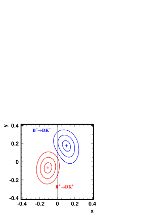
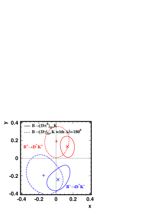
Figure 2: Results of the fits for $B^{-}\rightarrow DK^{-}$ (left) and $B^{-}\rightarrow D^{*}K^{-}$ (right) samples, where the contours indicate 1, 2, and 3 (left) and 1 (right) standard-deviation regions.

3 Result for $B^{-}\rightarrow DK^{-},~{}D\rightarrow K^{+}\pi^{-}$

The effect of $CP$ violation can be enhanced, if the final state of the $D$ decay following to the $B^{-}\rightarrow DK^{-}$ is chosen so that the interfering amplitudes have comparable magnitudes [8]. The decay $D\rightarrow K^{+}\pi^{-}$ is a particularly useful mode; the usual observables are the partial rate ${\cal R}_{DK}$ and the $CP$-asymmetry ${\cal A}_{DK}$ defined as

$${\cal R}_{DK} \equiv \frac{{\cal B}(B^{-}\rightarrow[K^{+}\pi^{-}]_{D}K^{-})+{\cal B}(B^{+}\rightarrow[K^{-}\pi^{+}]_{D}K^{+})}{{\cal B}(B^{-}\rightarrow[K^{-}\pi^{+}]_{D}K^{-})+{\cal B}(B^{+}\rightarrow[K^{+}\pi^{-}]_{D}K^{+})}$$ (3)

$$= r_{B}^{2}+r_{D}^{2}+2r_{B}r_{D}\cos{(\delta_{B}+\delta_{D})}\cos{\phi_{3}},$$

$${\cal A}_{DK} \equiv \frac{{\cal B}(B^{-}\rightarrow[K^{+}\pi^{-}]_{D}K^{-})-{\cal B}(B^{+}\rightarrow[K^{-}\pi^{+}]_{D}K^{+})}{{\cal B}(B^{-}\rightarrow[K^{+}\pi^{-}]_{D}K^{-})+{\cal B}(B^{+}\rightarrow[K^{-}\pi^{+}]_{D}K^{+})}$$ (4)

$$= 2r_{B}r_{D}\sin{(\delta_{B}+\delta_{D})}\sin{\phi_{3}}/{\cal R}_{DK},$$

where $[f]_{D}$ indicates that the state $f$ originates from a $D$ meson, $r_{D}=|A(D^{0}\rightarrow K^{+}\pi^{-})/A(D^{0}\rightarrow K^{-}\pi^{+})|$, and $\delta_{D}=\delta(D^{0}\rightarrow K^{-}\pi^{+})-\delta(D^{0}\rightarrow K^{+}\pi^{-})$. For the parameters $r_{D}$ and $\delta_{D}$, external experimental inputs can be used [9].

In this report, we show a preliminary result based on a data sample that contains $7.7\times 10^{8}$ $B\bar{B}$ pairs (the full data sample collected by Belle at $\Upsilon(4S)$ resonance). The decay $B^{-}\rightarrow D\pi^{-}$ is also analyzed similarly as a reference mode. For the largest background from the continuum process $e^{+}e^{-}\rightarrow q\bar{q}$, we apply the new method of the discrimination based on NeuroBayes neural network [10]. The inputs are a Fisher discriminant of modified Super-Fox-Wolfram moments, cosine of the decay angle of $D\rightarrow K^{+}\pi^{-}$, vertex separation between the reconstructed $B$ and the remaining tracks, and seven other variables. The signal is extracted by a two-dimensional fit on $\Delta E$ and NeuroBayes output ($\cal NB$), where we simultaneously fit for $DK^{-}$, $DK^{+}$, $D\pi^{-}$, and $D\pi^{+}$, as shown in Figure 3. As a result, we obtain

$${\cal R}_{DK} = [1.62\pm 0.42({\rm stat})^{~{}+0.16}_{~{}-0.19}({\rm syst})]\times 10^{-2},$$ (5)

$${\cal A}_{DK} = -0.39\pm 0.26({\rm stat})^{~{}+0.06}_{~{}-0.04}({\rm syst}),$$ (6)

$${\cal R}_{D\pi} = [3.28\pm 0.37({\rm stat})^{~{}+0.22}_{~{}-0.23}({\rm syst})]\times 10^{-3},$$ (7)

$${\cal A}_{D\pi} = -0.04\pm 0.11({\rm stat})^{~{}+0.01}_{~{}-0.02}({\rm syst}),$$ (8)

where the first evidence of the suppressed $DK$ signal is obtained with a significance $3.8\sigma$ including systematic error. Our study will make a significant contribution to a model-independent extraction of $\phi_{3}$ by combining relevant observables, e.g., the partial rates and the $CP$-asymmetries for $D\rightarrow CP$ eigenstates [11].

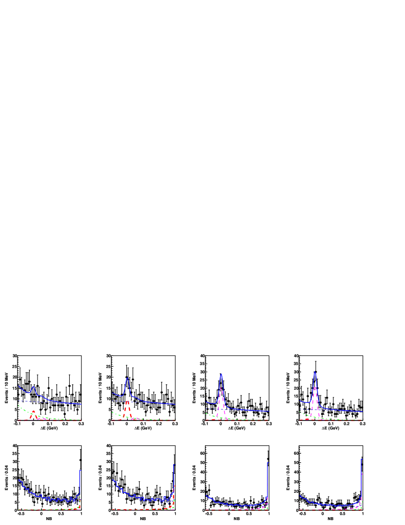
Figure 3: The distributions of $\Delta E$ for ${\cal NB}>0.5$ (top) and $\cal NB$ for $|\Delta E|<40~{}{\rm MeV}$ (bottom) on the suppressed modes $DK^{-}$, $DK^{+}$, $D\pi^{-}$, and $D\pi^{+}$ from left to right. The components are thicker long-dashed red ($DK$), thinner long-dashed magenta ($D\pi$), dash-dotted green ($B\bar{B}$ background), and dashed blue ($q\bar{q}$ background).

4 Conclusion

In conclusion, recent results on the decays $B^{-}\rightarrow D^{(*)}K^{-}$ followed by $D\rightarrow K_{S}\pi^{+}\pi^{-}$ and $D\rightarrow K^{+}\pi^{-}$ are reported. By the Dalitz-plot analysis for $D\rightarrow K_{S}\pi^{+}\pi^{-}$, the value of $\phi_{3}$ is measured to be $\phi_{3}=78.4^{\circ}~{}^{+10.8^{\circ}}_{-11.6^{\circ}}({\rm stat})\pm 3.6^{\circ}({\rm syst})\pm 8.9^{\circ}({\rm model})$. For $D\rightarrow K^{+}\pi^{-}$, preliminary results on the partial rate ${\cal R}_{DK}$ and the $CP$-asymmetry ${\cal A}_{DK}$ are reported, where the first evidence of the signal is obtained with a significance $3.8\sigma$.

References

[1]
N. Cabibbo, Phys. Rev. Lett. 10, 531 (1963).
[2]
M. Kobayashi and T. Maskawa, Prog. Theor. Phys. 49, 652 (1973).
[3]
L. Wolfenstein, Phys. Rev. Lett. 51, 1945 (1983).
[4]
A. Giri, Yu. Grossman, A. Soffer, and J. Zupan, Phys. Rev. D 68, 054018 (2003).
[5]
A. Bondar, Proceedings of BINP Special Analysis Meeting on Dalitz Analysis, 2002 (unpublished).
[6]
A. Poluektov et al. (Belle Collaboration), Phys. Rev. D 81, 112002 (2010).
[7]
A. Bondar, A. Poluektov, Eur. Phys. J. C 55, 51 (2008).
[8]
D. Atwood, I. Dunietz, and A. Soni, Phys. Rev. Lett. 78, 3257 (1997);
Phys. Rev. D 63, 036005 (2001).
[9]
HFAG, online update at http://www.slac.stanford.edu/xorg/hfag/charm.
[10]
M. Feindt, U. Kerzel, Nucl. Instrum. Methods Phys. Res., Sect. A 559, 190 (2006).
[11]
M. Gronau and D. Wyler, Phys. Lett. B 265, 172 (1991).