Continuous-variable quantum key distribution with Gaussian source noise

Abstract

Source noise affects the security of continuous-variable quantum key distribution (CV QKD), and is difficult to analyze. We propose a model to characterize Gaussian source noise through introducing a neutral party (Fred) who induces the noise with a general unitary transformation. Without knowing Fred’s exact state, we derive the security bounds for both reverse and direct reconciliations and show that the bound for reverse reconciliation is tight.

I INTRODUCTION

Continuous-variable quantum key distribution helps two remote parties (Alice and Bob) to establish a set of secret keys at high speed Scarani_RMP_09 . Different from discrete-variable protocols, in CV QKD Alice encodes information into the quadratures of the optical field and Bob decodes it with high-efficiency and high-speed homodyne detection GG02 ; Grosshans_Nature_03 ; Weedbrook_PRL_04 . Besides the experimental advantages and demonstrations, the security of CV QKD is also studied theoretically. The coherent-state CV-QKD protocol with Gaussian modulation has been proved secure under the collective attack Grosshans_PRL_05 ; Navascues_PRL_05 ; Garcia_PRL_06 ; Navascues_PRL_06 ; Piradola_PRL_08 , and the fact that the security bounds for collective and coherent attacks coincide asymptotically has been clarified using quantum De Finetti theorem Scarani_RMP_09 ; Renner_PRL_09 . However, the security of practical CV-QKD system has only been noticed recently Lodewick_PRA_10 ; Lodewick_Ex_PRA_07 . It has been observed that adding noise in the error-correction postprocessing may increase the secret key rate Garcia_PRL_09 . Furthermore, Filip et al. noticed that the source noise in coherent state preparation would undermine the key rate Filip_PRA_08 ; Filip_PRA_10 . More recently, Weedbrook et al. has shown that direct reconciliation CV protocols is more robust against this noise than reverse reconciliation protocols Weedbrook_PRL_10 .

From a practical viewpoint, it is meaningful to consider the trusted Gaussian source noise which is not controlled by the potential eavesdropper Eve. To analyze this source-noise effect, it is convenient to use the entanglement-based (EB) scheme to evaluate CV-QKD security. Note that two requirements for the EB scheme should be satisfied here. First, the EB scheme is kept equivalent to the practical prepare and measure (PM) scheme Grosshans_QIC_03 . Second, in the EB scheme the optimality of Gaussian attack is guaranteed under the collective attack. From this viewpoint, a three-mode entangled-state model has been proposed in Shen_JPB_09 as a preliminary attempt. However, the security bound in that paper is not tight, since in order to derive a calculable bound the model assumes that the source noise is untrusted, from which Eve is able to acquire extra information. Another attempt Filip_PRA_10 used a beam-splitter model [Fig. 1(a)], analogous to the realistic detector model Lodewick_Ex_PRA_07 , to characterize the source noise.

In this paper, we propose a novel EB model to characterize the Gaussian source noise. In this model a neutral party Fred introduces Gaussian source noise through a general Gaussian transformation. Without knowing Fred’s exact state, a security bound can be derived which is tighter than previous work Shen_JPB_09 . We also analyze the performance of the beam-splitter model under situations where source noise process includes either signal amplification or attenuation, and make comparisons with our result.

II MODEL DESCRIPTION

Before the explicit description of our model, the definition of the covariance matrix of a quantum state is briefly reviewed. For an N-mode quantum state, its covariance matrix $\gamma$ is defined by

$$\gamma_{ij}={\rm Tr}[\rho\{(\hat{r}_{i}-d_{i}),(\hat{r}_{j}-d_{j})\}],$$ (1)

where the operator vector is $\hat{r}=(\hat{x}_{1},\hat{p}_{1},\hat{x}_{2},\hat{p}_{2},\ldots,\hat{x}_{N},\hat{p}_{N})$ and the displacement vector is $d_{i}={\rm Tr}(\rho\hat{r}_{i})$ ($d\in\mathbb{R}^{2N}$). $\hat{x_{i}}$ and $\hat{p_{i}}$ are the quadratures of each optical field mode.

The EB scheme of the beam-splitter model and our model is illustrated in Fig. 1. In the beam-splitter model the source is characterized by an EPR state held by Alice. Then an extra EPR state interacts with either mode of the original one, depending on whether the source noise process amplifies or attenuates the signal, to introduce the noise. This is shown in Fig. 1(a) and Fig. 1(b).

Our model is demonstrated in Fig. 1(c) where the source is also characterized by an EPR state. Alice obtains the data by measuring one of mode $A$ and sends the other one $B_{0}$ to Bob as the signal. We assume that Gaussian source noise is introduced by Fred who implements a unitary Gaussian transformation over ${F_{0}}$ and the signal ${B_{0}}$. The covariance matrix of the Gaussian state $\rho_{FAB_{1}}$ describing Fred-Alice-Bob system after the transformation is

$$\gamma_{FAB_{1}}= \left(\begin{array}[]{cccc}F_{11}&F_{12}&F_{13}&F_{14}\\ F_{21}&F_{22}&F_{23}&F_{24}\\ F_{31}&F_{32}&V\mathbb{I}&\sqrt{T_{A}(V^{2}-1)}\sigma_{z}\\ F_{41}&F_{42}&\sqrt{T_{A}(V^{2}-1)}\sigma_{z}&T_{A}(V+\chi_{A})\mathbb{I}\\ \end{array}\right),$$ (6)

where $V$ is the variance of the EPR state, $T_{A}$ and $\chi_{A}$ characterize the influence of the Gaussian source noise on the signal mode, $\mathbb{I}$ is the $2\times 2$ identity matrix, $\sigma_{z}$ is the Pauli-z matrix, and each $F_{ij}$ represents an unknown $2\times 2$ matrix describing either $F$ or its correlations with $AB_{1}$.

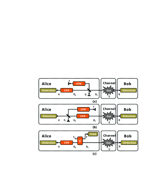
Figure 1: (a) Beam-splitter model with signal attenuation. An extra EPR state is presented and one mode of which is coupled with the signal mode to introduce the source noise. This is similar to the conventional detector model Lodewick_Ex_PRA_07 . (b) Beam-splitter model with signal amplification. The extra EPR state intervenes through coupling the mode sent to Alice and parameters are adjusted so that the EB scheme is equivalent to the PM scheme. (c) Our model. A neutral party Fred is presented who implements a unitary Gaussian transformation to introduce the source noise to the signal. The capital letters represent quantum states at each position.

With using the coherent-state protocol as an example, the equivalence between the EB scheme and the practical PM scheme is explained below. In the EB scheme Alice performs a heterodyne detection on her side and gets two measurement results $P_{A}$ and $X_{A}$. Bob’s state $\rho_{B_{1}}$ would be projected into a Gaussian state with covariance matrix $\gamma_{B_{1}}$ and mean $d_{B_{1}}$ satisfying Garcia PHD

$$\begin{split}\gamma_{B_{1}}&=T_{A}(\chi_{A}+1)\mathbb{I},\\ d_{B_{1}}=&\sqrt{\frac{2T_{A}(V-1)}{V+1}}(X_{A},-P_{A}).\end{split}$$ (8)

In the PM scheme Alice originally prepares the signal mode $B_{0}$ in a coherent state with displacement vector $d_{B_{1}}/{\sqrt{T_{A}}}$. Then, the effect of the source noise can be described by $\hat{p}_{B_{1}}=\sqrt{T_{A}}(\hat{p}_{B_{0}}+\delta_{P})$ and $\hat{x}_{B_{1}}=\sqrt{T_{A}}(\hat{x}_{B_{0}}+\delta_{X})$, in which $\delta_{P}$ and $\delta_{X}$ are uncorrelated noise terms with zero mean and variance $V(\delta_{P})=V(\delta_{X})=\chi_{A}$. The state sent to Bob is then identical to the one described in Eq. (8), indicating that source preparation in the real PM scheme can be properly characterized using the EB scheme. As the source-noise effect goes to zero, the equivalence would be identical to the one described in Grosshans_QIC_03 .

When the signal is sent through the channel, the attack of the potential eavesdropper Eve can be described as performing a unitary transformation $U_{BE}$ over the signal mode $B_{1}$ and her modes. After Eve’s interaction, the covariance matrix of the state $\rho_{FAB}$ would be

$$\gamma_{FAB}=$$

$$\left(\begin{array}[]{cccc}F_{11}&F_{12}&F_{13}&F_{14}^{\prime}\\ F_{21}&F_{22}&F_{23}&F_{24}^{\prime}\\ F_{31}&F_{32}&V\mathbb{I}&\sqrt{TT_{A}(V^{2}-1)}\sigma_{z}\\ F_{41}^{\prime}&F_{42}^{\prime}&\sqrt{TT_{A}(V^{2}-1)}\sigma_{z}&T[T_{A}(V+\chi_{A})+\chi]\mathbb{I}\\ \end{array}\right),$$ (13)

where $T$ and $\chi$ are channel parameters and $F_{ij}^{\prime}$ indicates the changed correlation terms due to Eve’s interaction. Note that since $\gamma_{FAB}$ is partly unknown but fixed, we can prove the optimality of Gaussian attack, as shown in Appendix A. In the following, the lower bounds on the secret key rate of this model would be derived without knowing the exact state of Fred in both reverse and direct reconciliations.

III REVERSE RECONCILIATION

In reverse reconciliation, the secret key rate is given by

$$K_{RR}=I(a:b)-S(b:E),$$ (15)

where $I(a:b)$ is classical mutual information between Alice and Bob and $S(b:E)$ is quantum mutual information between Bob and Eve. Given the above covariance matrix $\gamma_{FAB}$, $I(a:b)$ can be calculated from the reduced matrix $\gamma_{AB}$, while $S(b:E)$ can not be learned directly from $\gamma_{FAB}$ since $F_{ij}$ contains undetermined parameters. Fortunately, another Gaussian state $\rho_{FAB}^{\prime}$ with determined covariance matrix $\gamma_{FAB}^{\prime}$ exists, and serves as an upper bound on the calculation of the quantity $S(b:E)$. $\gamma_{FAB}^{\prime}$ has the form

$$\gamma_{FAB}^{\prime}=$$

$$\left(\begin{array}[]{cccc}I&0&0&0\\ 0&I&0&0\\ 0&0&T_{A}(V+\chi_{A})\mathbb{I}&\sqrt{T[T_{A}^{2}(V+\chi_{A})^{2}-1]}\sigma_{z}\\ 0&0&\sqrt{T[T_{A}^{2}(V+\chi_{A})^{2}-1]}\sigma_{z}&T[T_{A}(V+\chi_{A})+\chi]\mathbb{I}\\ \end{array}\right).$$ (20)

The relationship between two Gaussian states with $\gamma_{FAB}$ and $\gamma_{FAB}^{\prime}$ is explained below. Considering the pure Gaussian state $\rho^{\prime}_{FAB_{1}}$ with the covariance matrix

$$\gamma_{FAB_{1}}^{\prime}=$$

$$\left(\begin{array}[]{cccc}I&0&0&0\\ 0&I&0&0\\ 0&0&T_{A}(V+\chi_{A})\mathbb{I}&\sqrt{T_{A}^{2}(V+\chi_{A})^{2}-1}\sigma_{z}\\ 0&0&\sqrt{T_{A}^{2}(V+\chi_{A})^{2}-1}\sigma_{z}&T_{A}(V+\chi_{A})\mathbb{I}\\ \end{array}\right).$$ (26)

The reduced state $\rho^{\prime}_{B_{1}}=\mathrm{Tr}_{FA}(\rho^{\prime}_{FAB_{1}})$ is identical to the reduced state $\rho_{B_{1}}=\mathrm{Tr}_{FA}(\rho_{FAB_{1}})$, so $\rho^{\prime}_{FAB_{1}}$ and $\rho_{FAB_{1}}$ are two different purifications of this state. According to Nielsen_Chuang_BOOK_00 , one purification of a fixed system can be transformed into another through a local unitary transformation on its ancillary system. Hence there exists such a unitary map $U_{FA}$ that transforms $\rho_{FAB_{1}}$ to $\rho^{\prime}_{FAB_{1}}$. Furthermore, after taking Eve’s attack $U_{BE}$ into account and noticing that $U_{FA}$ and $U_{BE}$ commute, it can be proved that $\rho_{FAB}$ will be transformed into $\rho^{\prime}_{FAB}$ through $U_{FA}$.

In the rest of the paper expressions with the prime indicate the terms calculated by $\gamma^{\prime}_{FAB}$. The following lemma then allows us to bound Eve’s knowledge.

Lemma 1. Given two Gaussian states $\rho_{FAB}$ and $\rho^{\prime}_{FAB}$ with covariance matrices $\gamma_{FAB}$ and $\gamma^{\prime}_{FAB}$ shown in Eqs. (II) and (III), respectively, one has the equality

$$S(b:E)=S^{\prime}(b:E).$$ (28)

Proof. Based on $\gamma_{FAB}$ and $\gamma^{\prime}_{FAB}$ the mutual information between Bob and Eve is, respectively, given as

$$\begin{split}S(b:E)&=S(E)-S(E\mid b),\\ S^{\prime}(b:E)&=S^{\prime}(E)-S^{\prime}(E\mid b),\end{split}$$ (29)

where $S(E)$ and $S^{\prime}(E)$ are the von Neumann entropy of Eve’s state, and $S(E\mid b)$ and $S^{\prime}(E\mid b)$ are Eve’s entropy conditioned on Bob’s measurement results. $S(E)=S(F,A,B)$ and $S^{\prime}(E)=S^{\prime}(F,A,B)$ can be verified from the fact that Eve could purify the Fred-Alice-Bob system Garcia PHD . Because $\rho_{FAB}$ can be changed into $\rho^{\prime}_{FAB}$ through a unitary transformation $U_{FA}$, the von Neumann entropy $S(F,A,B)=S^{\prime}(F,A,B)$, and thus $S(E)=S^{\prime}(E)$. On the other hand, conditioning on Bob’s result $b$, the conditional state with $\gamma_{FA|B=b}$ can be transformed into the one with ${\gamma^{\prime}}_{FA|B=b}$ through $U_{FA}$, and thus $S(F,A\mid b)=S^{\prime}(F,A\mid b)$. Combining another fact that $S(E\mid b)=S(F,A\mid b)$ and $S^{\prime}(E\mid b)=S^{\prime}(F,A\mid b)$, we conclude that $S(b:E)=S^{\prime}(b:E)$.

$\Box$

Lemma 1 implies that calculation with $\gamma_{FAB}^{\prime}$ can bound Eve’s knowledge. Note that Eq. (28) is valid for protocols implementing either squeezed-state or coherent-state protocol with Bob using homodyne or heterodyne detection. Hence our model provides a tight security bound for all these protocols in reverse reconciliation.

IV DIRECT RECONCILIATION

Though direct reconciliation has the 3dB limit, the security bounds for the sqeezed-state protocol with homodyne detection and the no-switching protocol Weedbrook_PRL_04 are analyzed theoretically. In direct reconciliation, the secret key rate is given by

$$K_{DR}=I(a:b)-S(a:E).$$ (30)

$I(a:b)$ can be calculated from $\gamma_{AB}$, and $S(a:E)$ can be bounded by the following lemma.

Lemma 2. Given two Gaussian states $\rho_{FAB}$ and $\rho^{\prime}_{FAB}$ with covariance matrices $\gamma_{FAB}$ and $\gamma^{\prime}_{FAB}$, the following inequality can be verified

$$S(a:E)\leq S^{\prime}(a:E).$$ (31)

The proof can be seen in Appendix B. Note that the equality in Eq. (31) is achieved only when $F$ is independent of $E$, which is not necessarily satisfied in practice. This means that in order to bound the secret key rate, Eve’s knowledge about Alice is overestimated by using $S^{\prime}(a:E)$. Thus, the security bound derived here is not tight.

V NUMERICAL SIMULATION

Our simulation concerns the no-switching protocol in both reverse and direct reconciliations. The secret key rate $K_{DR}$ or $K_{RR}$ would depend on the variables $V$, $T_{A}$, $\chi_{A}$, $T$ and $\chi$ characterizing either source or channel influences. In the simulation the variance is set to $V=20$ and channel excess noise $\epsilon=T\chi-1+T=0.04$ close to the practical scenario Lodewick_Ex_PRA_07 , where electronic noise in Bob’s detection is simply treated as part of $\epsilon$. In addition, to analyze both signal attenuation and amplification cases the source parameters are set to $\epsilon_{A}=T_{A}\chi_{A}-1+T_{A}=0.1$ and $T_{A}=0.9$ or $T_{A}=1.1$ with regard to each process.

The secret key rate is calculated using our model, the untrusted source noise model, and the beam-splitter model. The mutual information $I(a:b)$ is calculated according to the protocol used, whose formula can be found in Garcia PHD . $S(a:E)$ and $S(b:E)$ in our model can be bounded using the simplified covariance matrix $\gamma^{\prime}_{FAB}$. To deal with the untrusted source noise, Fred is assumed to be part of Eve, and thus $S(a:E)$ and $S(b:E)$ are derived from $\gamma_{AB}$ Shen_JPB_09 . For the beam-splitter model the key rate is calculated with the covariance matrix including the ancillary modes, which is given in Eqs. (62) and (64) in Appendix C.

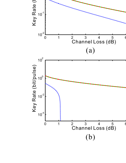
Figure 2: Secret key rate as a function of the transmittance of the channel in no-switching protocol with reverse reconciliation. The solid line stands for our model, dashed line for the beam-splitter model, and dotted line for the untrusted source noise model. Data are acquired under the variance of $V=20$, and channel’s excess noise is chosen to be $\epsilon=0.04$. (a) Signal attenuation with source parameter $T_{A}=0.9$ and $\epsilon_{A}=0.1$. (b) Signal amplification with source parameter $T_{A}=1.1$ and $\epsilon_{A}=0.1$

.

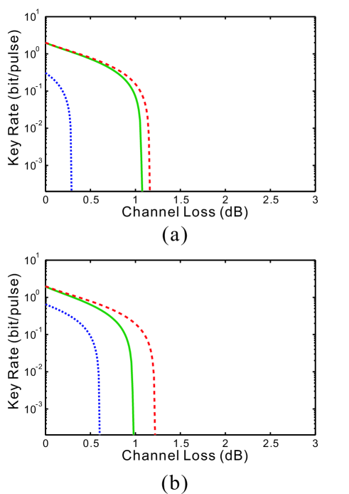
Figure 3: Secret key rate as a function of the transmittance of the channel in no-switching protocol with direct reconciliation. The solid line stands for our model, dashed line for the beam-splitter model, and dotted line for the untrusted source noise model. Data are acquired under the variance of $V=20$, and channel’s excess noise is chosen to be $\epsilon=0.04$. (a) signal attenuation with source parameter $T_{A}=0.9$ and $\epsilon_{A}=0.1$. (b) signal amplification with source parameter $T_{A}=1.1$ and $\epsilon_{A}=0.1$

.

VI DISCUSSION AND CONCLUSION

The simulation results can be seen in Figs. 2 and 3, where performances of our model, the beam-splitter model, and the untrusted source noise model are shown under no-switching protocol in reverse and direct reconciliations. From Figs. 2 and 3, it is clearly seen that the secret key rate of our model (solid line) coincides with that of the beam-splitter model (dashed line) in reverse reconciliation, while in direct reconciliation our result is lower. In addition, the security bound of our model is significantly higher than the untrusted source noise model (dotted line) in all cases.

In the reverse reconciliation case (as shown in Fig. 2) the coincidence of our model and the beam-splitter model on the secret key rate means that our model provides a tight security bound, even by generalizing Fred’s interaction. This coincidence is due to the fact that both models provide the same signal state, and the information leakage to Eve is estimated through this state. In the direct reconciliation shown in Fig. 3, we remark that our bound on the secret key rate can be further improved since the information gained by Eve is overestimated in mathematical treatment.

In conclusion, we have proposed a model to characterize the general Gaussian source noise in CV QKD. The result coincides with that of the beam-splitter model in reverse reconciliation protocols, proving that our generalized model can provide a tight bound on the secret key rate. In direct reconciliation, though the security bound is not tight, it still surpasses that of the untrusted source noise model in a significant way.

Appendix A Optimality of Gaussian Attack

Here, in our model, the security analysis on the optimality of Gaussian collective attack needs to be rechecked because the neutral party Fred is introduced in the EB scheme. Given the state $\rho_{FAB}$ with covariance matrix $\gamma_{FAB}$, it can be demonstrated that the security bound is obtained by considering Gaussian attack. The reason is listed as follows.

In Eqs. (15) and (30) $I(a:b)$ is lower bounded by Gaussian attack Navascues_PRL_06 . As for $S(a:E)$ in direct reconciliation, considering Bob and Fred together as a larger state $B^{*}$, thus $S(a:E)=S(E)-S(E\mid a)=S(A,B^{*})-S(B^{*}\mid a)$. According to Navascues_PRL_06 , $S(a:E)$ reaches its maximum when the quantum state $\rho_{AB^{*}}$ or $\rho_{FAB}$ is Gaussian, with covariance matrix $\gamma_{FAB}$. Therefore, Gaussian attack is optimal for direct reconciliation protocols. The deduction for the reverse reconciliation protocols follows a similar route.

Note that, in practical PM scheme, the source noise including light intensity fluctuation from a laser or modulator is a Gaussian one, thus the analysis is limited to the situation where Fred performs a general Gaussian transformation.

Appendix B Proof of Ineq. (11)

The mutual information between Alice and Eve is given by

$$\begin{split}S(a:E)&=S(E)-S(E\mid a),\\ S^{\prime}(a:E)&=S^{\prime}(E)-S^{\prime}(E\mid a),\end{split}$$ (32)

where the equation $S(E)=S^{\prime}(E)$ can be verified with similar reason demonstrated in Sec. III. Furthermore, we use the relations

$$S(E\mid a) \geq S(E\mid a,f),$$ (33)

$$S(E\mid a,f) \geq S^{\prime}(E\mid a,f),$$ (34)

$$S^{\prime}(E\mid a,f) = S^{\prime}(E\mid a),$$ (35)

where $S(E\mid a,f)$ ($S^{\prime}(E\mid a,f)$) means Eve’s entropy conditioned on the measurement results $a$ ($a^{\prime}$) and $f$ ($f^{\prime}$) of Alice and Fred. Here, Eq. (35) is obtained by noticing that in Eq. (III) Fred is uncorrelated with the rest of the system, that is, $\rho^{\prime}_{FABE}=\rho^{\prime}_{F}\bigotimes\rho^{\prime}_{ABE}$, so Nielsen_Chuang_BOOK_00

$$S^{\prime}(E\mid a,f) = S^{\prime}(E;a,f)-S^{\prime}(a,f)$$ (36)

$$= S^{\prime}(E;a)+S^{\prime}(f)-[S^{\prime}(a)+S^{\prime}(f)]$$

$$= S^{\prime}(E\mid a).$$

On the other hand, Eq. (33) holds because of the strong subadditivity of the von Neumann entropy Nielsen_Chuang_BOOK_00 . Furthermore, the equation

$$S(E\mid a,f)=S^{\prime}(E\mid a,f),$$ (37)

can be verified in the squeezed-state protocol with homodyne detection, while

$$S(E\mid a,f)\geq S^{\prime}(E\mid a,f),$$ (38)

holds in the no-switching protocol. Because both Gaussian states $\rho_{FABE}$ and $\rho^{\prime}_{FABE}$ are pure states, one has

$$\begin{split}S(E\mid a,f)&=S(B\mid a,f),\\ S^{\prime}(E\mid a,f)&=S^{\prime}(B\mid a,f).\end{split}$$ (39)

With using Eq. (39), Eq. (37) and InEq. (38) are explained below.

(1) In the squeezed-state protocol with homodyne detection, $S(B\mid a,f)=S^{\prime}(B\mid a,f)$ can be verified through proving $\gamma_{B}^{af}={\gamma^{\prime}}_{B}^{af}$, in which $\gamma_{B}^{af}$ (${\gamma^{\prime}}_{B}^{af}$) means the covariance matrix of the state $\rho_{B}$ ($\rho^{\prime}_{B}$) conditioning on the measurement results $a$ ($a^{\prime}$) and $f$ ($f^{\prime}$) of the state $\rho_{FA}$ ($\rho^{\prime}_{FA}$). The covariance matrix $\gamma_{B}^{af}$ can be obtained by Garcia PHD

$$\gamma_{B}^{af}=\gamma_{B}-\sigma_{B-FA}(X\gamma_{FA}X)^{MP}\sigma_{B-FA}^{T},$$ (40)

where $\sigma_{B-FA}$, $\gamma_{FA}$ and $\gamma_{B}$ denote part of $\gamma_{FAB}$

$$\gamma_{FAB}=\left(\begin{array}[]{cc}\gamma_{FA}&\sigma_{B-FA}^{T}\\ \sigma_{B-FA}&\gamma_{B}\\ \end{array}\right),$$ (41)

and $X$ is a matrix of the form

$$X=\left(\begin{array}[]{cccccc}1&0&0&0&0&0\\ 0&0&0&0&0&0\\ 0&0&1&0&0&0\\ 0&0&0&0&0&0\\ 0&0&0&0&1&0\\ 0&0&0&0&0&0\\ \end{array}\right),$$ (48)

which stands for the homodyne detection process on the $x$ quadrature. Note that the situation where the $p$ quadrature is measured has been omitted as its analysis would be identical to the $x$ quadrature case. The unitary transformation $U_{FA}$ corresponds in phase-space to a symplectic operation $S$ Garcia PHD , and therefore $\gamma_{FAB}^{\prime}=(S\bigoplus\mathbb{I}_{B})\gamma_{FAB}(S\bigoplus\mathbb{I}_{B})^{T}$. Combining Eq. (40), ${\gamma^{\prime}}_{B}^{af}$ would then be

$${\gamma^{\prime}}_{B}^{af}=\gamma_{B}-\sigma_{B-FA}S^{T}(XS\gamma_{FA}S^{T}X)^{MP}S\sigma_{B-AF}^{T}.$$ (49)

Without loss of generality, we assume $S$ takes a general form Garcia PHD

$$S=\left(\begin{array}[]{cccccc}a&0&b&0&c&0\\ 0&a^{\prime}&0&b^{\prime}&0&c^{\prime}\\ d&0&e&0&f&0\\ 0&d^{\prime}&0&e^{\prime}&0&f^{\prime}\\ g&0&h&0&i&0\\ 0&g^{\prime}&0&h^{\prime}&0&i^{\prime}\\ \end{array}\right),$$ (50)

and hence satisfying $SX=XS$. Therefore, one has

$$(XS\gamma_{AF}S^{T}X)^{MP} = (SX\gamma_{AF}XS^{T})^{MP}$$ (51)

$$= (S^{T})^{-1}(X\gamma_{AF}X)^{MP}(S)^{-1},$$

according to the characteristics of the Moore-Penrose pseudoinverse of matrix Isreal_Greville_BOOK_03 . Observing Eqs. (40), (49) and (51), $\gamma_{B}^{af}={\gamma^{\prime}}_{B}^{af}$, which means $S(B\mid a,f)=S^{\prime}(B\mid a,f)$. According to Eq. (39), the validity of Eq. (37) is proved.

(2) In the no-switching protocol, InEq. (38) is verified by comparing the explicit von Neumann entropy calculated from the two covariance matrices ${\gamma^{\prime}}_{B}^{af}$ and $\gamma_{B}^{af}$. Starting from $\rho^{\prime}_{FAB}$ , ${\gamma^{\prime}}_{B}^{af}$ can be written as Garcia PHD

$${\gamma^{\prime}}_{B}^{af} = \gamma_{B}^{\prime}-\sigma_{B-FA}^{\prime}(\gamma_{FA}^{\prime}+\mathbb{I})^{-1}\sigma^{\prime T}_{B-FA}$$

$$= \{T[T_{A}(V+\chi_{A})+\chi]-\frac{T[T_{A}^{2}(V+\chi_{A})^{2}-1]}{T_{A}(V+\chi_{A})+1}\}\mathbb{I},$$

where $\mathbb{I}$ is the 2$\times$2 identity matrix. On the other hand,

$$\gamma_{B}^{af}=\gamma_{B}^{\prime}-\sigma_{B-FA}^{\prime}(S^{-1})^{T}[S^{-1}\gamma_{FA}^{\prime}(S^{-1})^{T}+\mathbb{I}]^{-1}S^{-1}\sigma^{\prime T}_{B-FA}.$$

For the symplectic transformation $S^{-1}$, a decomposition of the form $S^{-1}=PS_{r}Q$ exists, which is known as the Bloch-Messiah reduction BM reduction . Here, $S_{r}$ is a squeezing operator on each mode

$$S_{r}=\left(\begin{array}[]{cccccc}e^{s_{1}}&0&0&0&0&0\\ 0&e^{-s_{1}}&0&0&0&0\\ 0&0&e^{s_{2}}&0&0&0\\ 0&0&0&e^{-s_{2}}&0&0\\ 0&0&0&0&e^{s_{3}}&0\\ 0&0&0&0&0&e^{-s_{3}}\\ \end{array}\right),$$ (54)

and $P$ and $Q$ stand for two passive transformations satisfying $P^{T}P=\mathbb{I}$ and $Q^{T}Q=\mathbb{I}$. Without loss of generality, matrix $Q$ takes a general form

$$Q=\left(\begin{array}[]{cccccc}a&0&b&0&c&0\\ 0&a^{\prime}&0&b^{\prime}&0&c^{\prime}\\ d&0&e&0&f&0\\ 0&d^{\prime}&0&e^{\prime}&0&f^{\prime}\\ g&0&h&0&i&0\\ 0&g^{\prime}&0&h^{\prime}&0&i^{\prime}\\ \end{array}\right).$$ (55)

With implementing the orthogonality of the passive transformation $P$, one has

$$\gamma_{B}^{af} = \gamma_{B}^{\prime}-\sigma_{B-FA}^{\prime}Q^{T}{S_{r}}^{T}(S_{r}Q\gamma_{FA}^{\prime}Q^{T}{S_{r}}^{T}+\mathbb{I})^{-1}S_{r}Q{\sigma_{B-FA}^{\prime}}^{T}$$ (58)

$$= T[T_{A}(V+\chi_{A})+\chi]\mathbb{I}-\left(\begin{array}[]{cc}\frac{T[T_{A}^{2}(V+\chi_{A})^{2}-1]}{T_{A}(V+\chi_{A})-1+\frac{1}{W}}&0\\ 0&\frac{T[T_{A}^{2}(V+\chi_{A})^{2}-1]}{T_{A}(V+\chi_{A})-1+\frac{1}{1-W}}\\ \end{array}\right),$$

where letter $W$ represents

$$\begin{split}W&=\frac{e^{2s_{1}}c^{2}}{e^{2s_{1}}+1}+\frac{e^{2s_{2}}f^{2}}{e^{2s_{2}}+1}+\frac{e^{2s_{3}}i^{2}}{e^{2s_{3}}+1},\\ 1-W&=\frac{c^{2}}{e^{2s_{1}}+1}+\frac{f^{2}}{e^{2s_{2}}+1}+\frac{i^{2}}{e^{2s_{3}}+1}.\end{split}$$ (60)

Using $Q^{T}Q=\mathbb{}{I}$, $W$ takes its value within $0<W<1$. To calculate its entropy, note that the von Neumann entropy of a Gaussian state $\rho$ is given by

$$S(\rho)=\sum_{i}g(\frac{\lambda_{i}-1}{2}),$$ (61)

where $g(x)=(x+1)\log_{2}(x+1)-x\log_{2}(x)$ and $\lambda_{i}$ is the symplectic eigenvalue of the covariance matrix of $\rho$. It can then be shown that the von Neumann entropy of $\gamma_{B}^{af}$ increases as its symplectic eigenvalue increases. Furthermore, the symplectic eigenvalue of $\gamma_{B}^{af}$ is the square of the multiplication of its diagonal entries, and the minimum of this eigenvalue is reached when $W=\frac{1}{2}$ in $\gamma_{B}^{af}={\gamma^{\prime}}_{F}^{af}$. This yields InEq. (38) in the no-switching protocol.

Appendix C Beam-Splitter Model under Gaussian Channel

The secret key rate of the beam-splitter model is to be calculated with signal attenuation or amplification, respectively. In case of attenuation ($T_{A}<1$) the model is shown in Fig. 1(a) Filip_PRA_10 and the result is obtained by setting the parameters in Eq. (II) as

$$\gamma_{FGAB}=\left(\begin{array}[]{cccc}N&\sqrt{T_{A}(N^{2}-1)}\sigma_{z}&0&-\sqrt{T(1-T_{A})(N^{2}-1)}\sigma_{z}\\ \sqrt{T_{A}(N^{2}-1)}\sigma_{z}&[T_{A}N+(1-T_{A})V]\mathbb{I}&\sqrt{(1-T_{A})(V^{2}-1)}\sigma_{z}&\sqrt{TT_{A}(1-T_{A})}(V-N)\mathbb{I}\\ 0&\sqrt{(1-T_{A})(V^{2}-1)}\sigma_{z}&V\mathbb{I}&\sqrt{TT_{A}(V^{2}-1)}\sigma_{z}\\ -\sqrt{T(1-T_{A})(N^{2}-1)}\sigma_{z}&\sqrt{TT_{A}(1-T_{A})}(V-N)\mathbb{I}&\sqrt{TT_{A}(V^{2}-1)}\sigma_{z}&T[T_{A}(V+\chi_{A})+\chi]\mathbb{I}\\ \end{array}\right),$$ (62)

where $N$ is the variance of the ancillary EPR’ shown in Fig. 1(a), which is related to the source parameters through $N=T_{A}\chi_{A}/(1-T_{A})$. Using this specific form of $\gamma_{FAB}$, Eve’s knowledge $S(E)-S(E\mid a)$ can be calculated by implementing the relation

$$S(E)-S(E\mid a)=S(FGAB)-S(FGB\mid a).$$ (63)

In case of amplification ($T_{A}>1$), one needs to modify the parameter setting, and change the model according to Fig. 1(b). Under this situation, the global covariance matrix reads

$$\gamma_{FGAB}=\left(\begin{array}[]{cccc}N_{B}&\sqrt{T_{B}(N^{2}_{B}-1)}\sigma_{z}&-\sqrt{(1-T_{B})(N^{2}_{B}-1)}\sigma_{z}&0\\ \sqrt{T_{B}(N^{2}_{B}-1)}\sigma_{z}&[T_{B}N_{B}+(1-T_{B})V_{B}]\mathbb{I}&\sqrt{T_{B}(1-T_{B})}(V_{B}-N_{B})\mathbb{I}&\sqrt{T(1-T_{B})(V^{2}_{B}-1)}\sigma_{z}\\ -\sqrt{(1-T_{B})(N^{2}_{B}-1)}\sigma_{z}&\sqrt{T_{B}(1-T_{B})}(V_{B}-N_{B})\mathbb{I}&T_{B}(V_{B}+\chi_{B})\mathbb{I}&\sqrt{TT_{B}(V^{2}_{B}-1)}\sigma_{z}\\ 0&\sqrt{T(1-T_{B})(V^{2}_{B}-1)}\sigma_{z}&\sqrt{TT_{B}(V^{2}_{B}-1)}\sigma_{z}&T(V_{B}+\chi)\mathbb{I}\\ \end{array}\right),$$ (64)

where $V_{B}=T_{A}(V+\chi_{A})$ is the modified variance of the EPR state, and the corresponding noise parameters are $T_{B}=T_{A}(V^{2}-1)/[T_{A}^{2}(V+\chi_{A})^{2}-1]$ and $\chi_{B}=[T_{A}^{2}(V+\chi_{A})(V\chi_{A}+1)-V]/[T_{A}(V^{2}-1)]$, leading to a modified variance of the ancillary EPR’ reading $N_{B}=T_{B}\chi_{B}/(1-T_{B})$. It is easy to verify that such replacement would lead to the same $\gamma_{AB}$ as in Eq. (II)

$$\gamma_{AB}= \left(\begin{array}[]{cc}T_{B}(V_{B}+\chi_{B})\mathbb{I}&\sqrt{TT_{B}(V^{2}_{B}-1)}\sigma_{z}\\ \sqrt{TT_{B}(V^{2}_{B}-1)}\sigma_{z}&T(V_{B}+\chi)\mathbb{I}\\ \end{array}\right)$$ (67)

$$= \left(\begin{array}[]{cc}V\mathbb{I}&\sqrt{TT_{A}(V^{2}-1)}\sigma_{z}\\ \sqrt{TT_{A}(V^{2}-1)}\sigma_{z}&T[T_{A}(V+\chi_{A})+\chi]\mathbb{I}\\ \end{array}\right),$$ (70)

and is therefore able to describe the amplification process. In order to make the model physical realizable, the parameters also need to satisfy $T_{B}<1$ and $\chi_{B}\geq(1-T_{B})/T_{B}$. The first inequality is easily recognized since now $T_{A}^{2}(V+\chi_{A})^{2}>T_{A}V^{2}$ and $T_{A}>1$, leading to $T_{A}(V^{2}-1)<T_{A}^{2}(V+\chi_{A})^{2}-1$. For the second inequality, by substituting $T_{A}$, $\chi_{A}$ and $V$ into it, we can transform it into

$$\chi_{A}^{2}+(V-1)\chi_{A}-\frac{(T_{A}V-1)(T_{A}-1)}{T_{A}^{2}}\geq 0.$$ (71)

Given that $\chi_{A}$ satisfies $\chi_{A}\geq(T_{A}-1)/T_{A}$ when $T_{A}>1$, it is easy to verify that the left hand side reaches its minimum when $\chi_{A}=(T_{A}-1)/T_{A}$, and the minimum is just 0, which proves the inequality.

With the above covariance matrix Eq. (64), Eve’s knowledge can be obtained.

References

• (1) V. Scarani, H. Bechmann-Pasquinucci, N. J. Cerf, M. Dušek, N. Lütkenhaus, and M. Peev, Rev. Mod. Phys. 81, 1301 (2009).
• (2) F. Grosshans and P. Grangier, Phys. Rev. Lett. 88, 057902 (2002).
• (3) F. Grosshans, G. Van Assche, J. Wenger, R. Brouri, N.J. Cerf, P. Grangier, Nature 421, 238 (2003).
• (4) C. Weedbrook, A. M. Lance, W. P. Bowen, T. Symul, T. C. Ralph, and P. K. Lam, Phys. Rev. Lett. 93, 170504 (2004).
• (5) F. Grosshans, Phys. Rev. Lett. 94, 020504 (2005).
• (6) M. Navascués, and A. Acín, Phys. Rev. Lett. 94, 020505 (2005).
• (7) R. García-Patrón and N. J. Cerf, Phys. Rev. Lett. 97, 190503 (2006).
• (8) M. Navascués, F. Grosshans, and A. Acín, Phys. Rev. Lett. 97, 190502 (2006).
• (9) S. Pirandola, S. L. Braunstein, and S. Lloyd, Phys. Rev. Lett. 101, 200504 (2008).
• (10) R. Renner and J. I. Cirac, Phys. Rev. Lett. 102, 110504 (2009).
• (11) J. Lodewyck et al., Phys. Rev. A. 76, 042305 (2007).
• (12) A. Leverrier, F. Grosshans, and P. Grangier, Phys. Rev. A. 81, 062343 (2010).
• (13) R. García-Patrón and N. J. Cerf, Phys. Rev. Lett. 102, 130501 (2009).
• (14) R. Filip, Phys. Rev. A 77, 022310 (2008).
• (15) V. C. Usenko and R. Filip, Phys. Rev. A 81, 022318 (2010).
• (16) C. Weedbrook, S. Pirandola, S. Lloyd, and T. Ralph, Phys. Rev. Lett. 105, 110501 (2010).
• (17) F. Grosshans, N. J. Cerf, J. Wenger, R. Tualle-Brouri, P. Grangier, Quantum Inf. Comput. 3, 535 (2003).
• (18) Y. Shen, J. Yang, and H. Guo, J. Phys. B: At. Mol. Opt. Phys. 42, 235506 (2009).
• (19) R. García-Patrón, Ph.D. thesis, Université Libre de Bruxelles, 2007.
• (20) M. A. Nielsen and I. L. Chuang, Quantum computation and quantum communication (Cambridge Univ. Press, Cambridge, 2000).
• (21) A. Ben-Israel and T. N. E. Greville, Generalized Inverses: Theory and Applications, Second Edition (Springer-Verlag, New York, 2003).
• (22) S. L. Braunstein, Phys. Rev. A. 71, 055801 (2005).