The luminosity function of Swift long gamma-ray bursts

Abstract

The accumulation of Swift observed gamma-ray bursts (GRBs) gradually makes it possible to directly derive a GRB luminosity function (LF) from observational luminosity distribution, where however two complexities must be involved as (i) the evolving connection between GRB rate and cosmic star formation rate and (ii) observational selection effects due to telescope thresholds and redshift measurements. With a phenomenological investigation on these two complexities, we constrain and discriminate two popular competitive LF models (i.e., broke-power-law LF and single-power-law LF with an exponential cutoff at low luminosities). As a result, we find that the broken-power-law LF could be more favored by the observation, with a break luminosity $L_{b}=2.5\times 10^{52}\rm erg~{}s^{-1}$ and prior- and post-break indices $\nu_{1}=1.72$ and $\nu_{2}=1.98$. For an extra evolution effect expressed by a factor $(1+z)^{\delta}$, if the matallicity of GRB progenitors is lower than $\sim 0.1Z_{\odot}$ as expected by some collapsar models, then there may be no extra evolution effect other than the metallicity evolution (i.e., $\delta$ approaches to be zero). Alternatively, if we remove the theoretical metallicity requirement, then a relationship between the degenerate parameters $\delta$ and $Z_{\max}$ can be found, very roughly, $\delta\sim 2.4(Z_{\max}/Z_{\odot}-0.06)$. This indicates that an extra evolution could become necessary for relatively high metallicities.

1 Introduction

Some confirmed associations between gamma-ray bursts (GRBs) and Type Ib/c supernovae (Stanek et al. 2003; Hjorth et al. 2003; Chornock et al 2010) robustly suggest that GRBs are powered by the collapse of the core of massive stars, which is also widely accepted in theory (Woosley 1993; Paczyński 1998; Fryer et al. 1999; Wheeler et al 2000; Woosley & Bloom 2006). In other words, the detection of each GRB provides a witness of the death of a massive star. Moreover, the intense brightness of GRBs makes them detectable even at the edge of the universe (the highest redshift of GRBs is $\sim 9.4$ as reported by Cucchiara et al. 2011). So GRBs can in principle be used as a tracer of the cosmic star formation history. The crucial problem is whether GRBs are an unbiased tracer or, more directly, how to calibrate GRB event rate to star formation rate (SFR). On one hand, the cosmic evolution of metallicity could be involved. This is because a very high angular momentum is required for GRB progenitors and meanwhile massive stars in lower-metallicity environments are less likely to loss much angular momentum through stellar winds (e.g., Meynet et al. 1994; Langer & Henkel 1995; Vink & de Koter 2005; MacFadyen & Woosley 1999; Wooseley & Heger 2006). On the other hand, the luminosity function (LF) of GRBs can also play an important role in the conversion from the observed GRB redshift distribution to GRB formation history, since the luminosity selection by telescopes leads to a lower detection probability for higher-redshift GRBs.

To directly derive a GRB LF was impossible before the launch of Swift (Gehrels et al. 2004), since there were only quite a few GRBs whose redshifts are measured. A possible alternative way invokes some luminosity-indicator relationships to avoid redshift measurements (e.g. Yonetoku et al. 2004; Fenimore & Ramirez-Ruiz 2000; Firmani et al. 2004), but the robustness of those indicators may be not high enough. A much more popular method is to assume a LF form with a few model parameters and then to fit the flux distribution of the observed GRBs ($\log N-\log P$ distribution; Schmidt 1999; Porciani & Madau 2001; Firmani et al. 2004; Guetta et al. 2005; Natarajan et al. 2005; Daigne et al. 2006; Salvaterra & Chincarini 2007; Salvaterra et al. 2009; Campisi et al. 2010). Correspondingly, before Swift, a very large sample of GRBs had been provided by the Burst and Transient Source Experiment (BATSE) on board Compton Observatory. Nevertheless, by such a fitting to $\log N-\log P$ distribution only, it is not easy to eliminate the degeneracy among the model parameters and even to determine the form of the LF. As a result, two competitive LF models as a broken-power law (BPL) and a single-power law with an exponential cutoff (SPLEC) at low luminosities are usually adopted in literature.

Thanks to Swift spacecraft, in the past few years the number of GRBs with measured redshift grows rapidly. This makes it possible to provide more stringent constraints on the LF parameters (Daigne et al. 2006; Salvaterra & Chincarini 2007; Salvaterra et al. 2009; Campisi et al. 2010). The new constraints robustly rule out the models in which GRBs unbiased trace the cosmic star formation or GRBs are characterized by a constant LF. In other words, an evolution effect is suggested. In view of the not-small size of the Swift GRB sample, it has become possible to derive a GRB LF only with Swift GRBs. Very recently, Wanderman & Piran (2010) tried to directly convert the luminosity distribution of Swift GRBs to a LF, without a prior assumed LF form and without a help from the BATSE data In such a LF-determination process, the treatments on observational selection effects play a very important role. Meanwhile, a possible extra evolution effect should also be paid much attention to. In this paper, with a phenomenological investigation on the evolution effect and the selection effects, we constrain and discriminate the BPL and SPLEC models by using Swift observed GRBs.

In the next section, some observational and theoretical materials related to the GRB LF are described. In section 3, the evolution effect is constrained and analyzed with relatively-high-luminosity GRBs. In Section 4, firstly, we derive an initial LF in both the BPL and SPLEC models by directly fitting the observational luminosity distribution of GRBs. Secondly, we analyze and constrain the so-called redshift-desert effect with the initial LFs. Finally, the combination of the above two processes gives a final constraint on the GRB LF, with which the prior selected luminosity threshold is checked. In Section 5, conclusion and discussion are given.

2 Basic materials

2.1 Swift observed GRBs

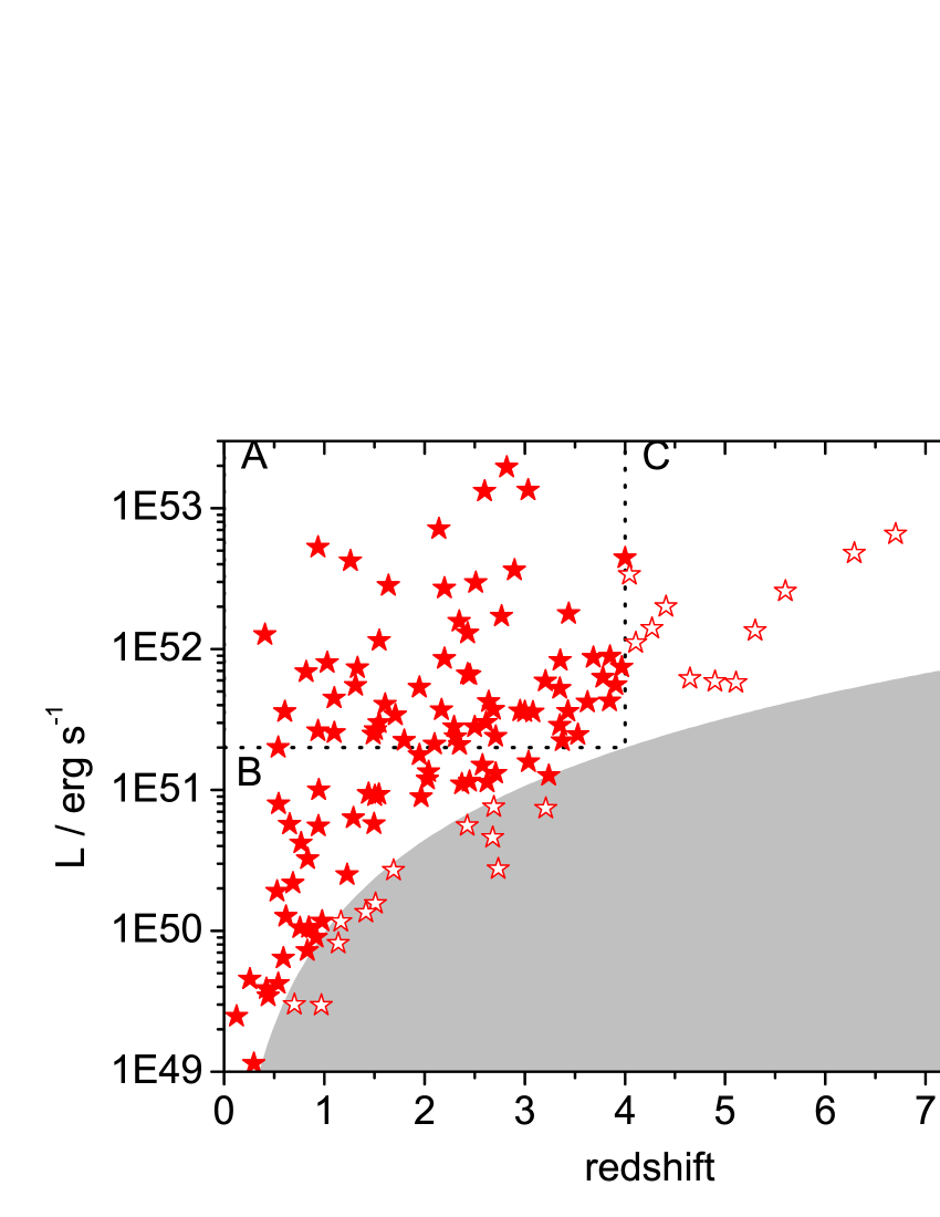
Figure 1: Luminosity-redshift distribution of 125 Swift GRBs with redshift, where the shaded region represents the luminosity threshold adopted in our calculations (see Equation 9 and explanations there). The 24 data labeled by open asterisks will be excluded from our most statistics.

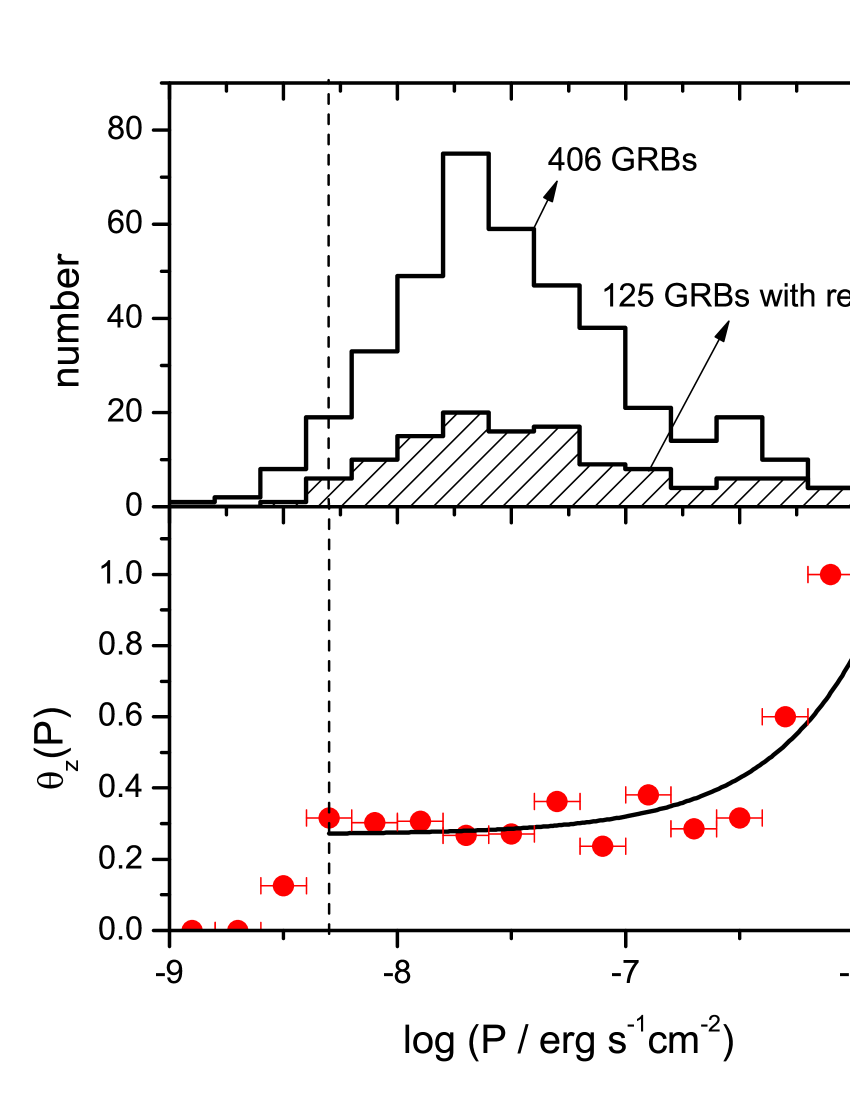
Figure 2: Upper panel: Comparison between the distributions of average fluxes of the total 406 GRBs and the 125 GRBs with redshift; Lower panel: Probability of redshift measurements as a function of flux and an empirical fitting given by Equation (2), where the horizon error bars correspond to the bin width. The vertical dashed line represents the selected threshold $P_{\rm th}=5\times 10^{-9}~{}\rm erg~{}s^{-1}cm^{-2}$.

In the past few years, Swift has greatly promoted our understanding of GRBs. Here we take GRBs with measured redshift $z$ from the Swift archive. For most of these GRBs till GRB 090813, their spectral peak energy $E_{p}$ and isotropically-equivalent energy release $E_{\rm iso}$ in the burst rest-frame $\rm 1-10^{4}~{}keV$ band have been provided by Butler et al. (2007, 2010). However, it should be noticed that, due to the narrow energy bandpass of the Swift Burst Alert Telescope (BAT), the burst spectral parameters in Butler et al. (2007, 2010) are actually estimated by the Bayesian statistics, but not directly observed. Anyway, as in Kistler et al. (2008, 2009) and Wang & Dai (2009), an average luminosity can be roughly estimated for these GRBs by

$$L_{[1-10^{4}\rm keV]}={E_{\rm iso[1-10^{4}\rm keV]}\over T_{90}/(1+z)}.$$ (1)

In our statistics, GRBs with $L<10^{49}\rm erg~{}s^{-1}$ will be excluded, since they may belong to a distinct population called low-luminosity GRBs (Soderberg et al. 2004; Cobb et al. 2006; Chapman et al. 2007; Liang et al. 2007). Finally, 125 GRBs are selected and their luminosity-redshift distribution is shown in Figure 1. Correspondingly, including the GRBs without redshift, there are totally 406 GRBs detected by Swift till GRB 090813.

In the upper panel of figure 2, we present the distributions of the observed average fluxes, $P_{[15-150\rm keV]}$, for both the total 406 GRBs and the 125 GRBs with redshift. The ratio between these two distributions generally displays the flux-dependence of the GRB redshift measurements and, as shown in the lower panel, such a redshift detection probability can be empirically expressed by

$$\vartheta_{z}(P)=\min\left[0.27+{P\over 2.0\times 10^{-6}\rm erg~{}s^{-1}cm^{-2}},1\right].$$ (2)

A similar result has also been given in Qin et al. (2010). On the other hand, the redshift detection probability may also depend on redshift itself, which will be investigated in section 4.2.

2.2 Model

The luminosity-redshift distribution of GRBs is determined by both the LF $\phi(L)$ and the comoving rate $\dot{R}(z)$ of GRBs, which are respectively defined by

$$\frac{d{N}}{dL}=\phi(L),$$ (3)

and

$$\frac{d\dot{N}}{dz}=\dot{R}(z)\frac{dV(z)/dz}{1+z},$$ (4)

where the dot represents time derivation, the factor $(1+z)$ is due to the cosmological time dilation of the observed rate and $dV(z)/dz$ is the comoving volume element. In the standard $\Lambda$-cold dark matter cosmology, $dV(z)/dz=4\pi d_{c}(z)^{2}c/H(z)$ with $d_{c}(z)=d_{l}(z)/(1+z)$, where the luminosity distance reads $d_{l}(z)=c(1+z)\int_{0}^{z}H(z^{\prime})^{-1}dz^{\prime}$ with $H(z^{\prime})=H_{0}[(1+z^{\prime})^{3}\Omega_{m,0}+\Omega_{\Lambda,0}]^{1/2}$. Throughout we adopt the cosmological parameters as $\Omega_{m,0}=0.27$, $\Omega_{\Lambda,0}=0.73$, and $H_{0}=71~{}\rm km~{}s^{-1}Mpc^{-1}$ (Komatsu et al. 2010).

Firstly, for the GRB rate $\dot{R}(z)$, it can in principle be connected to the cosmic SFR $\dot{\rho}_{*}(z)$, since in the collapsar model the formation of each GRB just indicates the death of a short-lived massive star. For relatively low redshifts ($z<4$), the SFR can be expressed approximately by (Hopkins & Beacom 2006)

$$\dot{\rho}_{*}(z)\propto\left\{\begin{array}[]{ll}(1+z)^{3.44},&z<0.97,\\ (1+z)^{-0.26},&0.97\leq z<4,\end{array}\right.$$ (5)

with $\dot{\rho}_{*}(0)=0.02~{}{\rm M_{\odot}yr^{-1}Mpc^{-3}}$, whereas the star formation history above $z\sim 4$ is unclear so far. So 12 GRBs with $z>4$ (the data in region C in Figure 1) are excluded from our statistics. Secondly, for the GRB LF, two representative forms are usually assumed in literature as a BPL

$$\phi(L)\propto\left\{\begin{array}[]{ll}\left({L\over L_{b}}\right)^{-\nu_{1}},&L\leq L_{b},\\ \left({L\over L_{b}}\right)^{-\nu_{2}},&L>L_{b}.\end{array}\right.,$$ (6)

and a SPLEC

$$\phi(L)\propto\left({L\over L_{p}}\right)^{\nu}e^{-L_{p}/L}.$$ (7)

Then the expected number of GRBs with redshift $z_{1}<z<z_{2}$ and luminosity $L_{1}<L<L_{2}$ can be calculated by

$$N^{\rm exp}\propto\int_{z_{1}}^{z_{2}}\int_{\max[L_{1},L_{\rm th}(z)]}^{L_{2}}(1+z)^{\Delta}\phi(L)\dot{\rho}_{*}(z)dL{dV(z)\over 1+z},$$ (8)

where the extra evolving factor $(1+z)^{\Delta}$ is introduced by considering that (i) the connection between the GRB rate and the SFR could be not in a trivial way and (ii) the LF could evolve with redshift. Corresponding to different selection criterions and bin methods for different GRB samples, the specific form of the above equation (e.g., the sequence and the range of the integrals) should be changed, see Equations (10), (11), (13), (15), and (18).

The luminosity threshold invoked in Equation (8) can be given by

$$L_{\rm th}(z)=4\pi d_{l}(z)^{2}P_{\rm th}k(z),$$ (9)

where $k(z)\equiv\int_{1\rm keV}^{10^{4}\rm keV}S(E^{\prime})E^{\prime}dE^{\prime}/\int_{15(1+z)\rm keV}^{150(1+z)\rm keV}S(E^{\prime})E^{\prime}dE^{\prime}$ (the primes represent rest-frame energy) converts the observed flux in the BAT energy band $\rm 15-150$ keV into the bolometric flux in the rest-frame $\rm 1-10^{4}$ keV. The observed photon number spectrum $S(E)$ can be well expressed by the empirical Band function (Band et al. 1993), more simply, a broken power law. The value of $k$ varies from 5.4 to 2.1 as the redshift increases from 0 to 10, by taking the rest-frame peak energy as $E^{\prime}_{p}\sim 200~{}{\rm keV}$ (the most frequent value in the Butler et al.’s database) and the photon indices prior and post the break energy as 1 and 2.25 , respectively (Preece et al. 2000). On the other hand, unfortunately, a precise description for $P_{\rm th}$ is nearly impossible, since the trigger of the BAT is very complicated and, especially for GRBs with redshift, the actual threshold is determined by the combination of the BAT and other related telescopes. Instead of an abrupt cutoff at $P_{\rm th}$, a realistic situation could be that the detection efficiency starts to remarkably decrease at a certain flux and approaches to be zero with decreasing fluxes. Therefore, in the following calculations, a relatively high value for $P_{\rm th}$ is taken as $5\times 10^{-9}~{}\rm erg~{}s^{-1}cm^{-2}$ and, correspondingly, 12 GRBs below the selected threshold are further excluded (as shown in Figure 1). Strictly speaking, the selected $P_{\rm th}$ is not but higher than the true sensitivity. This can make us avoiding the complex arising from the trigger probability. The availability of the selected $P_{\rm th}$ will be checked by a fitting to the $\log N-\log P$ distribution in section 4.3.

2.3 Observational luminosity distribution

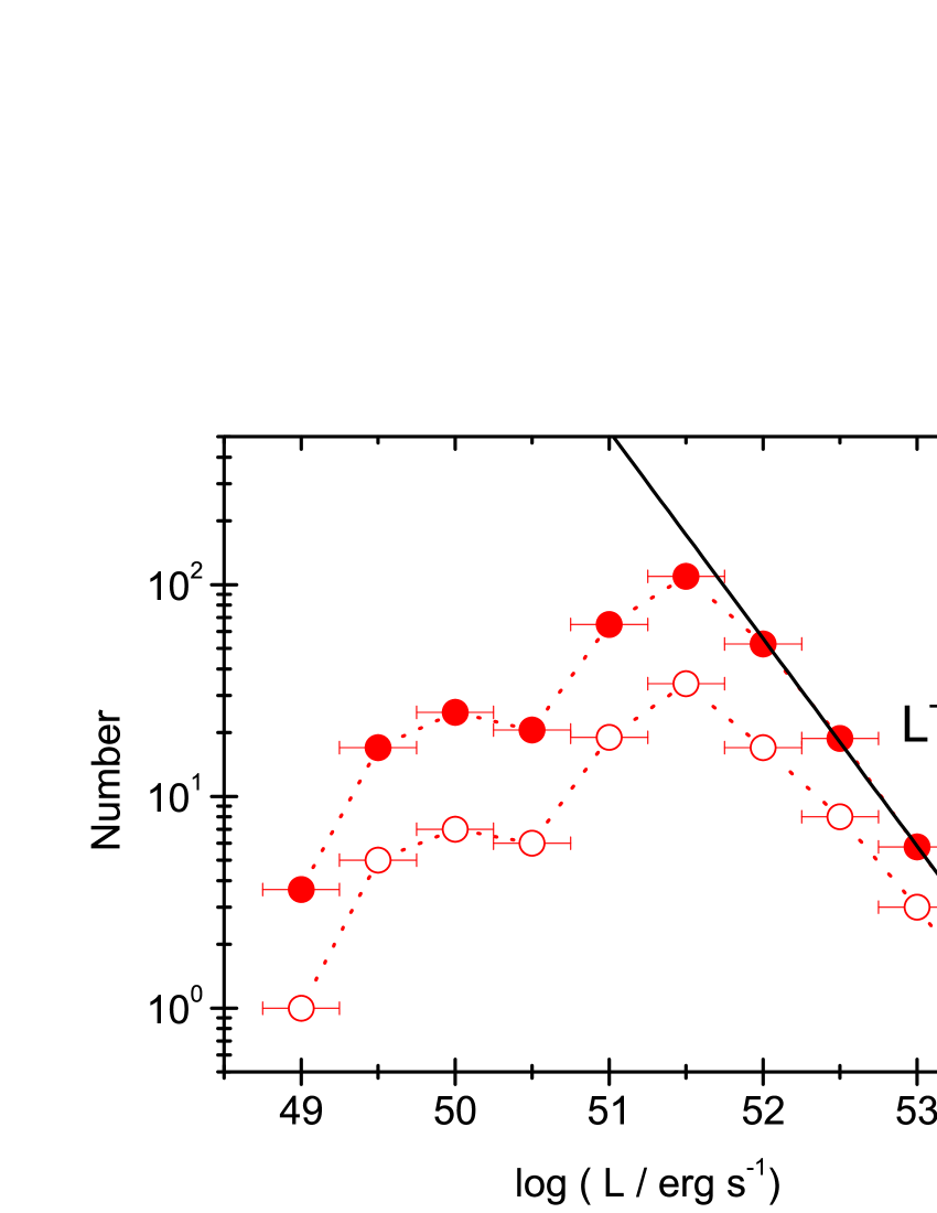
Figure 3: Luminosity distribution of the selected 101 GRBs, where the horizon error bars correspond to the bin width. Open and solid circles correspond to pre- and post-corrected distributions, respectively, and the solid line gives a power-law fitting for the corrected high-luminosity distribution. The equivalent number of the corrected sample is about 319.

As the main objective we want to account for, the luminosity distribution of the selected 101 GRBs (solid asterisks in Figure 1) is presented in Figure 3, where an obvious break appears at $\sim 3\times 10^{51}\rm erg~{}s^{-1}$. Such a break may reflect an intrinsic break in LF or just be caused by the selection effects arising from the BAT and also other related telescopes, which is what we want to clarify in this paper. In order to avoid the consideration of the flux-dependence of the redshift measurements in our analyses, we count an effective number as $\vartheta_{z}^{-1}(P)$ for each GRB with flux $P$ whose redshift is measured. As a result, an effective GRB sample of a number of about 319 is derived from the 101 GRBs. Since darker GRBs have higher weight in the statistics, the corrected luminosity distribution becomes steeper, especially above the break luminosity. A good power-law fitting as $N\propto L^{-0.98}$ to the high-luminosity distribution indicates $\nu_{2}=1.98$ in the BPL model and $\nu=1.98$ in the SPLEC model, in view of the probable unimportance of most observational selection effects at high-luminosity range. In the following Figures 4, 6, 7, and 8, the observational data are all with the same number correction.

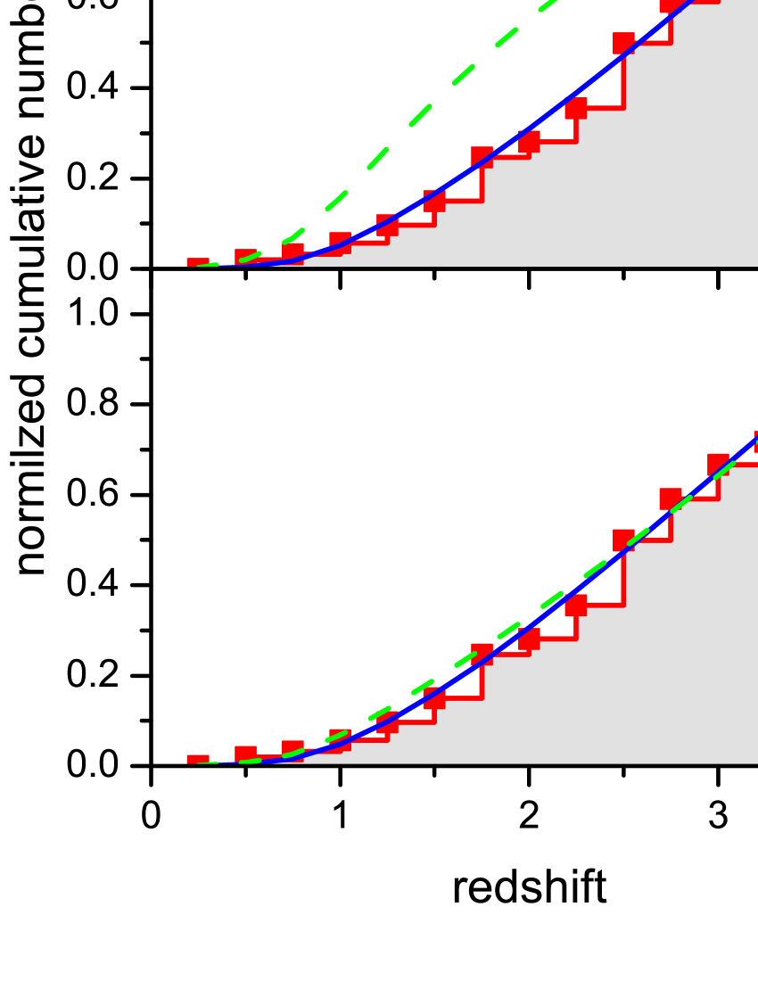
Figure 4: Normalized cumulative number of the 63 GRBs with $z<4$ and $L>2\times 10^{51}\rm erg~{}s^{-1}$ as a function of redshift (histogram). Upper panel: Fittings to the redshift distribution with Equation (10), where the solid and dashed lines correspond to $\Delta=1.93$ and $\Delta=0$, respectively. Lower panel: Fittings to the redshift distribution with Equation (11), where the solid and dashed lines correspond to $Z_{\max}=0.72Z_{\odot}$, $\delta=1.56$ (best fit) and $Z_{\max}=0.1Z_{\odot}$, $\delta=0$, respectively.

3 Evolution effect

Before we use the observational luminosity distribution to constrain the GRB LF with equation (8), we should determine the evolution parameter $\Delta$ in advance. Following Yüksel et al. (2008) and Kistler et al. (2009), the value of $\Delta$ can be constrained by fitting the observational cumulative redshift distribution of GRBs with relatively high luminosities ($L\geq L_{\rm cut}$). The cut luminosity $L_{\rm cut}$ is chosen to be equal to or higher than the threshold at the highest redshift of the sample (here $z_{\max}=4$), so that, in the corresponding theoretical calculation, the integral of the LF can be treated as a constant coefficient no matter the specific form of the LF, i.e.,

$$N^{\rm exp}_{<z}\propto\int_{L_{\rm cut}}^{L_{\max}}\phi(L)dL\int_{0}^{z}(1+z^{\prime})^{\Delta}\dot{\rho}_{*}(z^{\prime}){dV(z^{\prime})\over 1+z^{\prime}}.$$ (10)

Due to the limited size of the sample, the observational redshift distribution actually is slightly dependent on the selected $L_{\rm cut}$. So we take $L_{\rm cut}=L_{\rm th}(4)=2\times 10^{51}\rm erg~{}s^{-1}$ to reduce the statistical uncertainty as much as possible. Consequently, 63 GRBs (the data in region A in Figure 1) are selected. A comparison between the model and the observation is presented in the upper panel of Figure 4, which shows that the non-evolution case ($\Delta=0$) can be definitely ruled out, as found before (e.g., Salvaterra & Chincarini 2007; Salvaterra et al. 2009; Kistler et al. 2008, 2009). The best fitting to the observation gives $\Delta=1.93$.

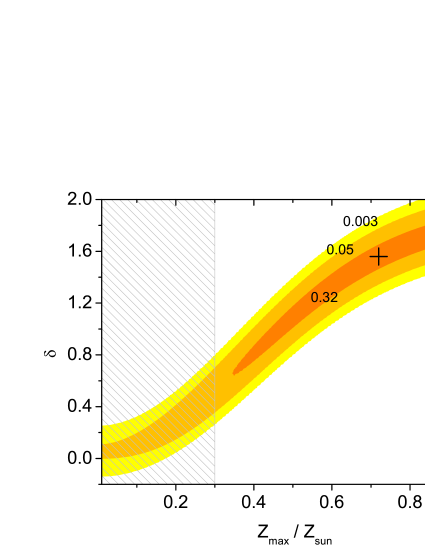
Figure 5: $\chi^{2}$-probability distribution of the fittings with Equation (11) to the redshift distribution of the 63 GRBs with $z<4$ and $L>2\times 10^{51}\rm erg~{}s^{-1}$. The best-fit parameters $\delta=1.56$ and $Z_{\max}=0.72Z_{\odot}$ is labeled by the cross. The hatched region represents the theoretical metallicity range expected by some collapsar models.

Then an interesting question arises as where such an evolution comes from. As found by MacFadyen & Woosley (1999) and Yoon et al. (2006), the formation of the black hole (or neutron star) during the collapse can drive a GRB event only if the collapsar has high angular momentum. In order to avoid strong stellar winds loosing angular momentum, GRB progenitors are required to be in low-metallicity evironments (Woosley & Heger 2006; Yoon et al. 2006). This theoretical metallicity requirement is widely favored by the estimations of the metallicities of long GRB hosts (e.g. Chen et al. 2005; Gorosabel et al. 2005; Starling et al. 2005). Therefore, it is suggested that the observationally required evolution could be mainly due to the cosmic evolution of metallicity. Specifically, as derived by Langer & Norman (2006), the fraction belonging to metallicity below $Z_{\max}$ can be calculated by $\Psi_{<Z_{\rm\max}}(z)={\left.\hat{\Gamma}[0.84,(Z_{\rm\max}/Z_{\odot})^{2}10^{0.3z}]\right./\Gamma(0.84)}$, where $Z_{\max}$ is the maximum metallicity available for GRB progenitors and $\hat{\Gamma}$ and $\Gamma$ are the upper incomplete and complete gamma functions. Following this consideration, Equation (10) becomes

$$N^{\rm exp}_{<z}\propto\int_{L_{\rm cut}}^{L_{\max}}\phi(L)dL\int_{0}^{z}(1+z^{\prime})^{\delta}\Psi_{<Z_{\rm\max}}(z^{\prime})\dot{\rho}_{*}(z^{\prime}){dV(z^{\prime})\over 1+z^{\prime}}.$$ (11)

Varying the parameters $Z_{\max}$ and $\delta$, we refit the observational redshift distribution shown in Figure 4 and present the distribution of the $\chi^{2}$-probabilities of the fittings in Figure 5. At first sight, the best-fit parameters $Z_{\rm\max}=0.72Z_{\odot}$ and $\delta=1.56$ may indicate that there is a significant extra evolution other than the metallicity evolution. However, the long and narrow contours shown in Figure 5 robustly demonstrate that the parameters $Z_{\max}$ and $\delta$ are actually strongly degenerate and, moreover, the specific values of the best-fit parameters are probably sensitive to the selection of the observational sample. Therefore, instead of paying attention to the best-fit parameters, we treat the relationship between the two parameters exhibited by the contours as a more valuable result, very roughly, $\delta\sim 2.4(Z_{\max}/Z_{\odot}-0.06)$. Anyway, an independent constraint on these two parameters is demanded in order to reduce the parameter degeneracy.

For example, a theoretical constraint on metallicity can be invoked (e.g., Campisi et al. 2010). As proposed by Woosley & Heger (2006) and Yoon et al. (2006), the maximum metallicity available for GRB progenitors is likely to be within $\sim[0.1-0.3]Z_{\odot}$. As shown in Figure 5, for $Z_{\max}<0.3Z_{\odot}$, the value of $\delta$ would not be higher than 0.8 with 99.7% confidence. Especially for $Z_{\max}<0.1Z_{\odot}$, the value of $\delta$ approaches to be zero. The fitting to the observation with $Z_{\max}=0.1Z_{\odot}$ and $\delta=0$ is shown in the lower panel of Figure 4 in comparison with the fitting with $Z_{\rm\max}=0.72Z_{\odot}$ and $\delta=1.56$. As can be seen, the difference between these two fittings is not very significant. Therefore, an extra evolution other than the metallicity evolution may be not inevitable if $Z_{\max}$ is indeed very low.

In the following calculations, we take the best-fit parameters $Z_{\max}=0.72$ and $\delta=1.56$ just for a good description for the evolution effect. Constraints on the LF actually can not be significantly affected by the variation of $Z_{\max}$ and $\delta$ as long as they satisfy the required relationship. On the other hand, for simplicity, we will ascribe the possible extra evolution to some unknown factors in the connection between the GRB rate and the SFR, i.e.,

$$\dot{R}(z)=C_{R}(1+z)^{\delta}\Psi_{<Z_{\max}}(z)\dot{\rho}_{*}(z),$$ (12)

where the proportional coefficient $C_{R}$ will be determined in Section 4.4. In other words, the LF will be taken to be non-evolving in this paper.

4 Luminosity function

4.1 A preliminary constraint

With given $Z_{\max}$ and $\delta$, we can constrain the unknown LF by fitting the observational luminosity distribution of the 101 GRBs by

$$N_{[L_{1},L_{2}]}^{\rm exp}\propto\int_{L_{1}}^{L_{2}}\int_{0}^{\min[z_{M}(L),4]}\phi(L)\dot{R}(z){dV(z)\over 1+z}dL,$$ (13)

which gives the expected number in each luminosity bin $L_{1}\leq L\leq L_{2}$. The maximum redshift $z_{M}(L)$ as a function of luminosity can be solved from

$$d_{l,M}(L) = {c(1+z)\over H_{0}}\int_{0}^{z_{M}}{1\over\sqrt{(1+z)^{3}\Omega_{m,0}+\Omega_{\Lambda,0}}}dz$$ (14)

$$= \left({L\over 4\pi P_{\rm th}k}\right)^{1/2}.$$

With fixed $\nu_{2}=1.98$ in the BPL model and $\nu=1.98$ in the SPLEC model and minimizing the $\chi^{2}$-statistic of the fittings, we obtain the best-fit parameters as $L_{b}=2.5\times 10^{52}\rm erg~{}s^{-1}$ and $\nu_{1}=1.67$ for the BPL model and $L_{p}=2.5\times 10^{49}\rm erg~{}s^{-1}$ for the SPLEC model. As shown in Figure 6, the fitting with a BPL LF seems much better than the one with a SPLEC LF. This impels us to favor the BPL model. However, the apparent oscillation of the observational data, which can not be explained by both models, still demands a much more elaborate fitting.

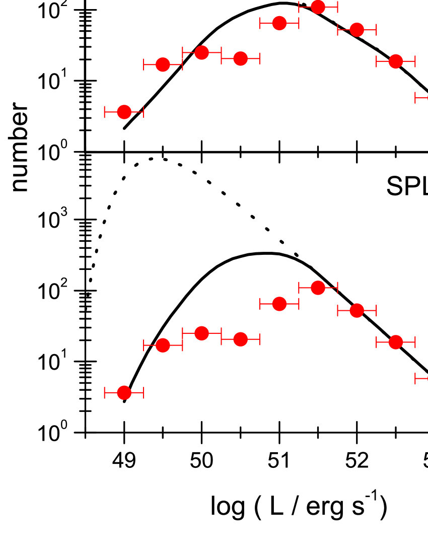
Figure 6: The best fitting to the observational GRB luminosity distribution with equation (13). The dotted and solid lines represent intrinsic and observable distributions, respectively. The parameters are $L_{b}=2.5\times 10^{52}\rm erg~{}s^{-1}$, $\nu_{1}=1.67$, and $\nu_{2}=1.98$ for the BPL model (upper) and $L_{p}=2.5\times 10^{49}\rm erg~{}s^{-1}$ and $\nu=1.98$ for the SPLEC model (lower).

4.2 Redshift-desert effect

With the preliminary LFs derived above, we can give some model-predicted cumulative redshift distributions by

$$N^{\rm exp}_{<z}\propto\int_{0}^{z}\int_{L_{\rm th}(z)}^{L_{\max}}\phi(L)\dot{R}(z^{\prime})dL{dV(z^{\prime})\over 1+z^{\prime}},$$ (15)

which are shown in the upper panel of Figure 7 in comparison with the observational one of the 101 GRBs. Obviously, the observational numbers at the middle redshifts are much less than the ones predicted by both the models. Such a remarkable dip in the observational redshift distribution is probably, at least partly, related to the so-called ‘redshift-desert’ effect, which is ignored in the above analyses. As qualitatively analyzed by Fiore et al. (2007), it could be difficult to measure redshifts within the range $1.1<z<2.1$, since at $z>1.1$ some strong observable emission or absorption lines are shifted outside the typical interval covered by optical spectrometers ($3800-8000{\AA}$) while Lyman-$\alpha$ enters the range at $z\sim 2.1$. In this paper we do not try to give a theoretical description for the redshift-desert effect, which must involve many physical and technical issues. We also notice that a same significant dip actually can not be found in the redshift distribution of only GRBs with $L>2\times 10^{52}\rm erg~{}s^{-1}$, as shown in Figure 4. Hence, we suspect that the redshift-desert effect may mainly influence the redshift measurements of relatively dark GRBs, which can also be implied by the luminosity distribution.

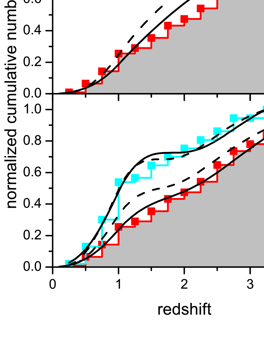
Figure 7: Model-predicted redshift distributions with (upper) and without (lower) redshift-desert effect in comparison with the observational distribution, where the adopted LFs are the same to Figure 6. The parameters for the redshift-desert effect read $\mu=1.80$ and $\sigma=0.79$ for the BPL model and $\mu=1.63$ and $\sigma=0.61$ for the SPLEC model.

Therefore, we show the observational redshift distribution of only 38 GRBs with $z<4$ and $L<2\times 10^{51}\rm erg~{}s^{-1}$ (the data in region B in Figure 1) in the lower panel of Figure 7. Meanwhile, for relatively dark GRBs, we tentatively suggest a Gaussian function

$$\eta_{z}(z)=1-\exp\left[-{(z-\mu)^{2}\over\sigma^{2}}\right]$$ (16)

to phenomenologically describe the redshift-dependence of the redshift measurements. In contrast, for sufficiently bright GRBs, we take

$$\eta_{z}(z)=1.$$ (17)

Fittings to the distribution of the 38 GRBs give the best-fit parameters as $\mu=1.80$ and $\sigma=0.79$ for the BPL model and $\mu=1.63$ and $\sigma=0.61$ for the SPLEC model, which are basically consistent with the theoretical expectation of the redshift-desert effect. With these phenomenological expressions of $\eta_{z}(z)$, we refit the redshift distribution of the 101 GRBs, which is also shown in the lower panel of Figure 7. As can be seen, the fittings are greatly improved, as the observational dip in the redshift distribution is produced naturally, especially in the BPL model.

4.3 Final results

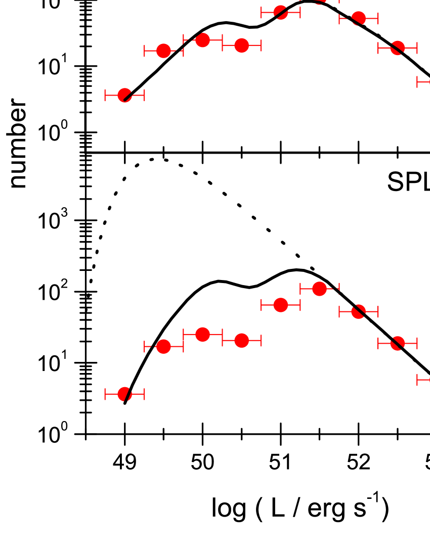
Figure 8: The same to Figure 6 but with a redshift-desert effect derived from Figure 7. The LF parameters are $L_{b}=2.5\times 10^{52}\rm erg~{}s^{-1}$, $\nu_{1}=1.72$, and $\nu_{2}=1.98$ for the BPL model and $L_{p}=2.5\times 10^{49}\rm erg~{}s^{-1}$ and $\nu=1.98$ for the SPLEC model.

Combining Equations (13), (16), and (17), we refit the luminosity distribution of the 101 GRBs and find that $L_{b}=2.5\times 10^{52}\rm erg~{}s^{-1}$ and $\nu_{1}=1.72$ for the BPL model and $L_{p}=2.5\times 10^{49}\rm erg~{}s^{-1}$ for the SPLEC model. Strictly, we should use these new LFs to re-constrain the redshift-desert effect and go recycling until reaching a certain precision. For simplicity, we stop here because the obtained new values of the parameters are only slightly different from the preliminary ones. With these new parameters, Figure 8 shows that the BPL model complies with the observation successfully, whereas the SPLEC model still predicts some remarkable excesses around $\sim 10^{50}-10^{51}\rm erg~{}s^{-1}$. Therefore, we prefer to conclude that the GRB LF could be a BPL.

Finally, with the derived BPL LF, we give a model-predicted cumulative flux distribution by

$${N^{\rm exp}_{>P}\propto\int_{0}^{4}\int_{L_{P}}^{L_{\max}}\phi(L)\dot{R}(z)\vartheta_{z}(P^{\prime})\eta_{z}(z)dL{dV(z)\over 1+z}},$$ (18)

where $L_{P}=4\pi d_{l}^{2}kP$, $P^{\prime}=L/4\pi d_{l}^{2}k$, and the redshift detection probability $\vartheta_{z}(P^{\prime})\eta_{z}(z)$ has been determined above. As shown in Figure 9, the consistency between the theoretical and observational flux distributions indicates that our choice of the luminosity threshold is basically reasonable, i.e., the trigger probability above $P_{\rm th}$ by the BAT can be affirmed to nearly constant.

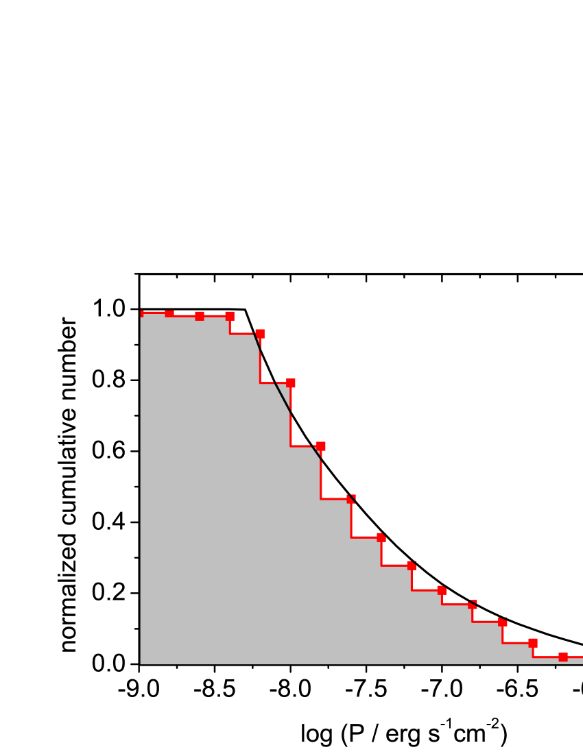
Figure 9: Comparison of the model-predicted flux distribution in the BPL LF model with the observational one (without number correction) of the 101 GRBs. The model parameters are the same to Figure 8.

4.4 GRB rate

In the above fittings to the luminosity distribution, we normalize the model-predicted GRB number by the following equation:

$$N_{[{53.25},{53.75}]}^{\rm obs} = {\Delta\Omega\over 4\pi}Tf_{b}\int_{{10^{53.25}}}^{10^{53.75}}C_{L}\phi(L)dL\int_{0}^{4}\dot{R}(z){dV(z)\over 1+z}.$$

where $(\Delta\Omega/4\pi)\sim 0.1$ is the field of view of the BAT, $T\sim 5$ yr is the observational period, $f_{b}\sim 0.01$ is the beaming degree of the GRB outflow, and $C_{L}\approx{(\nu_{1}-1)}\left({L_{\min}\over L_{b}}\right)^{\nu_{1}-1}{1\over L_{b}}$ is the normalization coefficient of the BPL LF with $L_{\min}$ being an assumed minimum luminosity for the GRBs.

For $\delta=1.56$, $Z_{\max}=0.72Z_{\odot}$, $\nu_{1}=1.72$, $\nu_{2}=1.98$, $L_{b}=2.5\times 10^{52}\rm erg~{}s^{-1}$, and $N_{[{53.25},{53.75}]}^{\rm obs}=1.9$, the proportional coefficient in the GRB rate can be constrained to

$$C_{R}=4\times 10^{-6}\left({L_{\min}\over 10^{-4}L_{b}}\right)^{1-\nu_{1}}\left({f_{b}\over 0.01}\right)^{-1}M_{\odot}^{-1},$$ (20)

which yields a overall local GRB rate as $\dot{R}(0)=C_{R}\Psi_{<Z_{\max}}(0)\dot{\rho}_{*}(0)=36(f_{b}/0.01)^{-1}~{}\rm Gpc^{-3}yr^{-1}$ and an observed local GRB rate as $f_{b}\dot{R}(0)=0.36~{}\rm Gpc^{-3}yr^{-1}$. This rate is basically consistent with the previous results (e.g., Schmidt 2001; Guetta et al. 2004, 2005; Liang et al. 2007; Wanderman & Piran 2010). The value of $C_{R}$ also implies that, besides the metallicity requirement, GRB progenitors may also have some other particularities. For example, as widely accepted, only massive Wolf-Rayet stars (e.g., $>20M_{\odot}$) are possible GRB progenitors (MacFadyen & Woosley 1999; Larsson et al. 2007). So a small fraction arises as $f_{\rm WR}=\left.\int_{20M_{\odot}}^{100M_{\odot}}\varphi(m)dm\right/\int_{0.1M_{\odot}}^{100M_{\odot}}m\varphi(m)dm\approx 2\times 10^{-3}~{}M_{\odot}^{-1}$, where $\varphi(m)$ is the Salpeter initial stellar mass function. Additionally, there is still an extra factor of $\sim 10^{-3}-10^{-2}$ unexplained, which could be related to the particularity of GRB progenitors in their rotation, magnetic fields, etc.

5 Conclusion and discussion

The accumulation of Swift observed GRBs gradually makes it possible to directly derive a GRB LF from observational luminosity distribution, where however two complexities must be involved as (i) the evolving connection between the GRB rate and the cosmic SFR and (ii) observational selection effects. With a phenomenological investigation on these two complexities, we constrain and discriminate two popular competitive LF models and find that the BPL LF model is more favored by the observation. However, in view of the approximative description of the selection effects, the SPLEC still can not be ruled out absolutely.

Although the derived values of the parameters $\mu$ and $\sigma$ are basically consistent with the theoretical expectation of the redshift-desert effect, the flux-dependence of the redshift-desert effect is still very ambiguous (an abrupt luminosity boundary as $2\times 10^{51}\rm erg~{}s^{-1}$ is adopted in our analyses). More seriously, the flux- and redshift-dependences of the redshift measurements actually must be coupled with each other, but in our analyses the functions $\vartheta_{z}(P)$ and $\eta_{z}(z)$ are considered independently for simplicity. This may lead to an overestimation of the redshift selection effect. Therefore, some more elaborate theoretical considerations on the redshift measurements are demanded. On the other hand, of course, a more detailed analysis on the observational results would be helpful, specially towards to every kind of redshift measurement methods.

Finally, our investigation on the evolution effect shows that, if the matallicity of GRB progenitors is lower than $\sim 0.1Z_{\odot}$ as expected by some collapsar models, there may be no extra evolution effect (i.e., $\delta\sim 0$) other than the metallicity evolution. Alternatively, if we remove the theoretical metallicity requirement, a stronger extra evolution would be required for higher metallicties. In the latter case, the extra evolution could indicate some other evolutions in the GRB rate or indicate an evolving LF which is not considered in this paper. To discriminate these two possibilities is difficult but interesting. It will be helpful to separate the GRB sample into few subsamples with different redshift ranges and fit the luminosity distribution of each subsamples one by one with an evolving LF. Such a further work can be made as the GRB sample becomes large enough.

References

- [1] Band, D., Matteson, J., Ford, L., et al. 1993, ApJ, 413, 281
- [2] Butler, N. R., Bloom, J. S., Poznanski, D. 2010,ApJ, 711, 495
- [3] Butler, N. R., Kocevski, D., Bloom, J. S., Curtis, J. L. 2007, ApJ, 671, 656
- [4] Campisi, M. A., Li, L.-X., Jakobsson, P. 2010, MNRAS,407, 1972
- [5] Chapman, R., Tanvir, N. R., Priddey, R. S., Levan, A. J. 2007, MNRAS, 382, L21
- [6] Chen H.-W., Prochaska J. X., Bloom J. S., Thompson I. B., 2005, ApJ, 634, L25
- [7] Chornock, R., Berger, E., Levesque, E. M., Soderberg, A. M., Foley, R. J., Fox, D. B., Frebel, A., Simon, J. D., et al. 2010, arXiv: 1004.2262
- [8] Cobb, B. E., Bailyn, C. D., van Dokkum, P. G., Natarajan, P. 2006, ApJ, 645, L113
- [9] Cucchiara, A., et al. 2011, ApJ, accepted, arXiv: 1105.4915
- [10] Daigne, F., Rossi, E. M., Mochkovitch, R. 2006, MNRAS, 372, 1034
- [11] Fenimore, E.E., Ramirez-Ruiz, E. 2000, arXiv: astro-ph/0004176
- [12] Firmani, C., Avila-Reese, V., Ghisellini, G., Tutukov, A. V. 2004, ApJ, 611, 1033
- [13] Fiore, F., Guetta, D., Piranomonte, S., D’Elia, V., Antonelli, L. A. 2007, A&A, 470, 515
- [14] Fryer, C. L., Woosley, S. E., & Hartmann, D. H. 1999, ApJ, 526, 152
- [15] Gehrels, N., Chincarini, G., Giommi, P., Mason, K. O., Nousek, J. A., Wells, A. A., White, N. E., Barthelmy, S. D., et al. 2004, ApJ, 611, 1005
- [16] Gorosabel J., Pérez-Ramírez, D., Sollerman, J., de Ugarte Postigo, A., Fynbo, J. P. U., Castro-Tirado, A. J., Jakobsson, P., Christensen, L., et al. 2005, A&A, 444, 711
- [17] Guetta, D., Perna, R., Stella, L., & Vietri, M. 2004, ApJ, 615, L73
- [18] Guetta, D., Piran, T., & Waxman, E. 2005, ApJ, 619, 412
- [19] Hjorth, J., Sollerman, J., Møller, P., Fynbo, J. P. U., Woosley, S. E., Kouveliotou, C., Tanvir, N. R., Greiner, J., et al. 2003, Nature, 423, 847
- [20] Hopkins, A. M., & Beacom, J. F. 2006, ApJ, 651, 142
- [21] Kistler, M. D., Yüksel, H., Beacom, J. F., Hopkins, A. M., Wyithe, J. Stuart B. 2009, ApJ, 705, 104
- [22] Kistler, M. D., Yüksel, H., Beacom, J. F., Stanek, K. Z. 2008, ApJ, 673, L119
- [23] Komatsu, E., Smith, K. M., Dunkley, J., Bennett, C. L., Gold, B., Hinshaw, G., Jarosik, N., Larson, D., et al. 2011, ApJS, 192, 18
- [24] Langer, N., Henkel, C. 1995, Space Science Reviews, 74, 343
- [25] Langer, N., Norman, C. A. 2006, ApJ, 638, L63
- [26] Larsson, J., Levan, A. J., Davies, M. B., Fruchter, A. S. 2007, MNRAS, 376, 1285
- [27] Liang, E., Zhang, B., Virgili, F., & Dai, Z. G. 2007, ApJ, 662, 1111
- [28] MacFadyen, A. I., & Woosley, S. E. 1999, ApJ, 524, 262
- [29] Meynet, G., Maeder, A., Schaller, G., Schaerer, D., Charbonnel, C. 1994, A&AS, 103, 97
- [30] Natarajan, P., Albanna, B., Hjorth, J., Ramirez-Ruiz, E., Tanvir, N., Wijers, R. 2005. MNRAS, 364, L8
- [31] Paczyński, B. 1998, ApJ, 494, L45
- [32] Porciani, C., & Madau, P. 2001, ApJ, 548, 522
- [33] Preece, R. D., Briggs, M. S., Mallozzi, R. S., Pendleton, G. N., Paciesas, W. S., Band, D. L. 2000, ApJSS, 126, 19
- [34] Qin S. F., Liang E. W., Lu R. J., Wei J. Y., Zhang S. N. 2010, MNRAS, 406, 558
- [35] Salvaterra, R., & Chincarini, G. 2007, ApJ, 656, L49
- [36] Salvaterra, R., Guidorzi, C., Campana, S., Chincarini, G., Tagliaferri, G. 2009, MNRAS, 396, 299
- [37] Schmidt, M. 1999, ApJ, 523, L117
- [38] Schmidt, M. 2001, ApJ, 552, 36
- [39] Soderberg, A. M., Kulkarni, S. R., Berger, E., Fox, D. W., Sako, M., Frail, D. A., Gal-Yam, A., Moon, D. S., et al. 2004, Nature, 430, 648
- [40] Starling R. L. C., Vreeswijk, P. M., Ellison, S. L., Rol, E., Wiersema, K., Levan, A. J., Tanvir, N. R., Wijers, R. A. M. J., et al., 2005, A&A, 442, L21
- [41] Stanek, K. Z., Matheson, T., Garnavich, P. M., Martini, P., Berlind, P., Caldwell, N., Challis, P., Brown, W. R., et al. 2003, ApJ, 591, L17
- [42] Vink, J.S., & de Koter, A. 2005, A&A, 442, 587
- [43] Wanderman, D. & Piran, T. 2010, MNRAS, 406, 1944
- [44] Wang, F. Y. & Dai, Z. G. 2009, MNRAS, 400, L10
- [45] Wheeler, J., et al. 2000, ApJ, 537, 810
- [46] Woosley, S. E., & Heger A., 2006, ApJ, 637, 914
- [47] Woosley, S. E., & Bloom, J. S. 2006, ARA&A, 44, 507
- [48] Woosley, S. E. 1993, ApJ, 405, 273
- [49] Yonetoku, D., Murakami, T., Nakamura, T., Yamazaki, R., Inoue, A. K., Ioka, K. 2004, ApJ, 609, 935
- [50] Yoon, S.-C., Langer, N., Norman, C. 2006, A&A, 460, 199
- [51] Yüksel, H., Kistler, M. D., Beacom, J. F., Hopkins, A. M. 2008, ApJ, 683, L5