Robust Dynamical Recurrences Based on Floquet Spectrum

Abstract

Recurrence behavior of wave packets in coupled higher dimensional systems and periodically driven systems is analyzed, which takes place in the realm of higher coupling/modulation strength. We analyze the wave packet dynamics close to nonlinear resonances developed in the systems and provide the analytical understanding of recurrence times. We apply these analytical results to investigate the recurrence times of matter waves in optical lattice in the presence of external periodic forcing. The obtained analytical results can experimentally be observed using currently available experimental setups.

1 Introduction

In one dimensional quantum systems with discrete energy spectrum, quantum recurrence theorem establishes the existence of recurrent dynamics PR1957 . Quantum characteristics of dynamical systems, which exhibit chaos in their classical domain, have posed interesting questions for researchers. These systems in general display inherent quantum interference phenomena which modify the quantum dynamics and produces a contrast in their evolution. Quantum interference phenomena, constructive or destructive in nature, contribute to the quantum recurrences in dynamical systems. Dynamical recurrences in such systems originate from the simultaneous excitation of discrete quasi-energy states  SaifPR . These recurrences are suitable to use as a probe to study quantum chaos ReinhardtBlumel2001 ; SaifPRE ; Saif2005-a . In this contribution we extend the discussion on the quantum recurrence phenomena and treat them in higher coupling/strong modulation regimes and study the quantum dynamics of the system for the nonlinear resonances. Our theoretical work is based on Floquet theory SIChuPR2004 , which presents an elegant formalism for the analysis of periodically driven and coupled higher dimensional systems RobertPRA2002 . Floquet state formalism has been applied to a number of time-dependent problems: from coherent states of driven Rydberg atom VelaPRA2005 , chaotic quantum ratchets HurPRA2005 , electron transmission in semiconductor hetero-structures ZhangPRB2006 , selectively suppressing of tunneling in quantum-dot array VillasPRB2004 to frequency-comb laser fields SonPRA2008 . The Floquet states have also been used in Bose-Einstein condensate systems and applied to probe superfluid-insulator transition Eckardt , towards coherent control HolthausPRA2001 and dynamical tunneling HensingerPRA2004 .

In this paper: (i) We extend Floquet analysis for nonlinear resonances and explain the existence of robust dynamical recurrences in dynamical system, in contrast to delicate dynamical recurrences already reported Saif2005-a ; SaifPR ; Saif2002 ; ShahidPLA ; (ii) Super revival times in dynamical systems are discussed first time for both delicate dynamical recurrences and robust dynamical recurrences; (iii) We show that, the non-linearity of the uncoupled systems, and the initial conditions on the excitation contribute to the classical period, quantum revival time and super revival time occurring in the coupled higher-dimensional systems or periodically driven systems; (iv) We apply these results to the dynamics of matter waves in driven optical lattices, a topic of current research Applications ; KurnNature2008 ; PottingPRA2001 . Classical dynamics of the system display an intricate dominant regular and dominant stochastic dynamics, one after the other, as a function of increasing modulation amplitude Bardroff1995 ; Raizen1999 .

The paper is organized as follows: The effective Hamiltonians for nonlinear resonances in higher dimensional systems (Sec. 2.1) and periodically driven time dependent systems (2.2) are derived. In Sec. 3, we explain the time scales and their dependence on system parameters. We apply obtained results to the matter wave dynamics in driven optical lattices and explain the time scales as a function of system parameters. We compare analytical and numerical results in Sec. 4.

2 Floquet Theory of Nonlinear Resonances

Floquet theory is an elegant formalism to quantize coupled higher dimensional systems (HDS) and periodically driven system (PDS) RobertPRA2002 . In HDS, with two degrees of freedoms coupled, such as Billiards Lenz2010 and in PDS, we observe various dynamical modes. In these Hamiltonian dynamical systems the stable nonlinear resonances are immersed in stochastic sea and the system may display global stochasticity beyond a critical value of coupling or modulation strength Lichtenberg ; LindaReichl ; E.Ott . Here, we apply Floquet analysis to find quasi energy eigen states and quasi energy eigen values in HDS and PDS and discuss their parametric dependencies on the uncoupled system and coupling constant or modulation strength.

2.1 Higher Dimensional Systems

We write general Hamiltonian for a system, with its degrees of freedom coupled, that is,

$$H=H_{0}(I)+\lambda H_{c}(I,\theta),$$ (1)

where, $H_{0}$ is the Hamiltonian of the system in the absence of coupling, expressed in the action coordinates $I=(I_{1},I_{2})$. Moreover, $H_{c}$ is the coupling Hamiltonian which describes coupling and is periodic in angle, $\theta=(\theta_{1},\theta_{2})$ and the parameter $\lambda$ is coupling strength. The Hamiltonian may express Billiard systems Lenz2010 in general systems and same time is a good candidate to describe multi-atomic molecule GoulvenPRA2011 and Lorentz gas Oliveira . We express the coupling Hamiltonian as,

$$H_{c}=\sum_{n}H_{n}(I)e^{i{n}.\theta},$$ (2)

where, $n=(n_{1},n_{2})$. Whenever, the frequencies $\Omega=\partial{H_{0}}/\partial I$ obey the relation, $n.\Omega=n_{1}\Omega_{1}+n_{2}\Omega_{2}=0$, resonances occur in the system.

We consider that the coupling exists between actions $I_{1}$ and $I_{2}$. Within the region of resonance, we find slow variations in action, hence, following the method of secular perturbation theory, we average over faster frequency, and get the averaged Hamiltonian for the $N^{th}$ resonance, as ${\bar{H}}={\bar{H}}_{0}(I)+\lambda V\cos(N\varphi_{-})$. Here, $\varphi_{-}=\theta_{1}-(M/N)\theta_{2}$, $I=I_{1}$ is the action corresponding to the angle $\theta_{1}$, $V$ is the Fourier amplitude, and $M$ and $N$ are relatively prime integers Lichtenberg . Averaging over rapidly changing $\varphi_{+}$ makes the corresponding action $I_{2}$ as the constant of motion. Moreover, ${\bar{H}}_{0}(I)$ expresses uncoupled averaged Hamiltonian.

The energy of initially narrowly peaked excitation changes slowly when we produce it in the vicinity of $N^{th}$ non-linear resonance. Therefore, we expand the unperturbed energy, ${\bar{H}}_{0}(I)$, by means of Taylor expansion around mean action $I=I_{0}$ and keep only the terms up to second order Flatte .

We Berry ; Almeida use operator definition of action, that is, $I=\frac{k^{-}}{i}\frac{\partial}{\partial\theta}$ to get the near resonant energy spectrum of the system by mapping the corresponding Schrödinger equation on the Mathieu equation SaifEPJD , where, the new variable $\theta=N\varphi/2$, hence, we get

$$[\frac{\partial^{2}}{\partial{\theta}^{2}}+a-2q\cos 2\theta]\phi(\theta)=0,$$ (3)

where, the Mathieu characteristic parameter AbramowitzStegun ; McLachlan , is

$$a=\frac{8}{N^{2}\zeta{k^{-}}^{2}}[{\mathcal{E}-\bar{H}}_{0}+\frac{\omega^{2}}{2\zeta}].$$ (4)

and

$$q=\frac{4\lambda V}{N^{2}\zeta{k^{-}}^{2}}.$$ (5)

The parameter $\zeta$ defines the nonlinear dependence of the energy of the system on the quantum number and $k^{-}$ is re-scaled Plank’s constant.

The $\pi$-periodic solutions of equation (3) correspond to even functions of the Mathieu equation whose corresponding eigenvalues are real AbramowitzStegun . These solutions are defined by Floquet states, i.e. $\phi(\theta)=e^{i\mu\theta}P_{\mu}(\theta)$, where, $P_{\mu}(\theta)=P_{\mu}(\theta+\pi)$, and $\mu$ is the characteristic exponent. In order to write the $\pi$-periodic solutions in $\varphi$-coordinate, we require $\mu$ to be defined as $\mu=\mu(j)=2j/N$, where, $j=0,1,2,....,N-1$.

The allowed values of $\mu(j)$ can exist as a characteristic exponent of solution to the Mathieu equation for discrete $\nu$ (which takes integer values) only for certain value $a_{\nu}(\mu(j),q)$, when $q$ is fixed. Hence, with the help of Eq. (4), we obtain the values of unknown $\mathcal{E}$. Therefore, we may express the eigen energy of the system as Holthaus1991

$$\mathcal{E}_{\mu,\nu}=\left[\frac{N^{2}{k^{-}}^{2}\zeta}{8}a_{\nu}(\mu(j),q)+k^{-}\alpha{j}+\bar{H}_{0}(I_{0})\right]\,\mathrm{mod}\,\,k^{-}\omega.$$ (6)

Here, $\alpha=M/N$ defines the winding number.

In order to check this result we study the case of zero coupling strength, that is $\lambda=0$. In this case, the value for Mathieu characteristic parameter becomes $a_{\nu}(q=0)={\nu}^{2}$. This reduces the quasi-energy $\mathcal{E}_{\mu,\nu}$, in the absence of coupling term, that is, $\lambda=0$, provided $\nu$ as $2(I-I_{0})/Nk^{-}$.

2.2 Time Dependent Systems

In the periodically driven potentials energy is no more a constant of motion. For the reason we solve the time dependent Schrödinger equation by using secular perturbation approximation as suggested by Max Born Born . Therefore, the solution is obtained by averaging over rapidly changing variables. This leads us to find out a partial solution of the periodically driven systems. As a result, we find quasi energy eigen-states and the quasi eigen energies of the dynamical system for non-linear resonances.

In order to study the quantum nonlinear resonance of the TDS, we consider the Hamiltonian,

$$H=H_{0}+\lambda V(x)\sin(t).$$ (7)

The solution of the Schrödinger equation corresponding to the Hamiltonian (7) can be written in the form  Saif2002 ; Flatte ; GPBerman1977 ,

$$|\psi(t)\rangle=\sum_{n}C_{n}(t)|n\rangle\exp\{-i[E_{\bar{n}}+(n-\bar{n})\frac{k^{-}}{N}]\frac{t}{k^{-}}\}.$$ (8)

Here, $E_{\bar{n}}$ is the mean energy, $C_{n}(t)$ is time dependent probability amplitude, $\bar{n}$ is mean quantum number and $|n\rangle$ are eigen states of undriven system. On substituting equation (8) in the time dependent Schrödinger equation, we find that the probability amplitude $C_{n}(t),$ changes with time following the equation, $ik^{-}{\dot{C}}_{n}(t)=[E_{n}-E_{\bar{n}}-(n-\bar{n})\frac{k^{-}}{N}]C_{n}(t)+\frac{\lambda V}{2i}(C_{n+N}-C_{n-N}).$ Where, $V=V_{n-N}\approx V_{n+N}$ are off-diagonal matrix elements and are approximately constant near the potential minima for tight-binding approximations.

We take the initial excitation, narrowly peaked around the mean value, $\bar{n}$. For the reason, we take slow variations in the energy, $E_{n}$, around the $\bar{n}$ in a nonlinear resonance, and expand it up to second order in Taylor expansion. Thus, the Schrödinger equation for the probability amplitudes, $C_{n}(t)$, is

$$ik^{-}{{\dot{C}}_{n}} =k^{-}(n-\bar{n})(\omega-\frac{1}{N})C_{n}(t)+\frac{1}{2}k^{-}(n-\bar{n})^{2}\zeta C_{n}(t)$$

$$+\frac{\lambda V}{2i}(C_{n+N}-C_{n-N}).$$ (9)

In order to obtain equation (9), we average over the fast oscillating terms and keep only the resonant ones. Here, the frequency, $\omega=\frac{\partial E_{n}}{k^{-}\partial n}|_{n=\bar{n}},$ and the non-linearity, in the time independent system is given as $\zeta=\frac{\partial^{2}E_{n}}{k^{-2}\partial n^{2}}|_{n=\bar{n}}.$

We introduce the Fourier representation for $C_{n}(t)$ as,

$$C_{n}(t)=\frac{1}{2N\pi}\int_{0}^{2N\pi}g(\theta,t)e^{-i(n-\bar{n})\theta/N}d\theta,$$ (10)

which helps us to express equation (9) as the Schrödinger equation for $g(\theta,t)$, such that $ik^{-}{\dot{g}}(\theta,t)=H(\theta)g(\theta,t)$. Here, the Hamiltonian $H(\theta)$ is given as, $H(\theta)=-\frac{N^{2}k^{-2}\zeta}{2}\frac{\partial^{2}}{\partial\theta^{2}}-iNk^{-}(\omega-\frac{1}{N})\frac{\partial}{\partial\theta}-\lambda V\sin\theta$. In order to obtain this equation, we consider the function $g(\theta,t)$ as $2N\pi$ periodic, in $\theta$ coordinate.

Due to the time-independent behavior of the Hamiltonian, we write the time evolution of $g(\theta,t)$, as $g(\theta,t)=\tilde{g}(\theta)e^{\frac{-i\varepsilon t}{k^{-}}}$. Therefore, Schrödinger equation for $g(\theta,t)$ reduces to the standard Mathieu equation (3). Here, we express $\tilde{g}=\chi(z)\exp\left(-i2(N\omega-1)z/N^{2}\zeta k^{-}\right)$, where, $\theta=2z+\pi/2$. The same as in equation (3), the Mathieu characteristic parameter, $a$, is defined as

$$a=\frac{8}{N^{2}k^{-2}\zeta}[\frac{(N\omega-1)^{2}}{2N\zeta}+\mathcal{E_{\mu,\nu}}],$$ (11)

$$\text{and \ \ \ \ \ \ \ }q=\frac{4\lambda V}{N^{2}k^{-2}\zeta}.$$ (12)

Hence, the quasi eigen energy of the system, obtained from equation (11), is

$$\mathcal{E}_{\mu,\nu}=\left[\frac{N^{2}k^{-2}\zeta}{8}a_{\nu}(\mu(j),q)+k^{-}\alpha{j}\right]\,\,\mathrm{mod}\,\,k^{-}\omega,$$ (13)

where, the index $\nu$ takes the definition, $\nu=\frac{2(n-\bar{n})}{N}$, where, $n$ is the quantum number for time independent system.

3 Quantum Revival Times Based on Quasi Energy Spectrum

In this section we discuss two cases correspond to nonlinear resonances. We consider weakly coupled $q<1$ or strongly coupled $q\gg 1$ potentials. In $q<1$ situation, for large $\nu$ Saif2002 and in $q\gg 1$ situation for small $\nu$, near the center of resonance matrix elements are constant. In the following discussion, we analyze the wave packet dynamics in these regimes and show their parametric dependencies.

The time scales, $T^{(j)}$ at which recurrences of an initially well-localized wave packet occur depend on the quasi-energy of the respective system, The recurrence times are obtained as, $T^{(j)}=2\pi/\Omega^{(j)}$, hence, the values of $j$ as $j=1,2,3...$, correspond to, respectively, classical, quantum, super, and higher order revival times. With the help of Eqs. (6) and (13), we obtain the frequencies $\Omega^{(j)}$ as

$$\Omega^{(1)} =\frac{1}{k^{-}}\left\{\frac{\partial\mathcal{E}_{\mu,\nu}}{\partial\mu}+\frac{\partial\mathcal{E}_{\mu,\nu}}{\partial\nu}\right\}$$

$$\Omega^{(2)} =\frac{1}{2!k^{-2}}\left\{\frac{\partial^{2}\mathcal{E}_{\mu,\nu}}{\partial\mu^{2}}+\frac{2\partial^{2}\mathcal{E}_{\mu,\nu}}{\partial\mu\partial\nu}+\frac{\partial^{2}\mathcal{E}_{\mu,\nu}}{\partial\nu^{2}}\right\}$$ (14)

$$\Omega^{(3)} =\frac{1}{3!k^{-3}}\left\{\frac{\partial^{3}\mathcal{E}_{\mu,\nu}}{\partial\mu^{3}}+3\frac{\partial^{3}\mathcal{E}_{\mu,\nu}}{\partial\mu^{2}\partial\nu}+3\frac{\partial^{3}\mathcal{E}_{\mu,\nu}}{\partial\mu\partial\nu^{2}}+\frac{\partial^{3}\mathcal{E}_{\mu,\nu}}{\partial\nu^{3}}\right\}.$$

After a few mathematical steps Eqs. (14) reduce to

$$\Omega^{(1)} =\frac{1}{k^{-}}\left\{\frac{\partial\mathcal{E}_{\mu,\nu}}{\partial\nu}+\alpha k^{-}\right\}$$

$$\Omega^{(2)} =\frac{1}{2!k^{-2}}\left\{\frac{\partial^{2}\mathcal{E}_{\mu,\nu}}{\partial\nu^{2}}+\alpha k^{-}\frac{2\partial\mathcal{E}_{\mu,\nu}}{\partial\nu}\right\}$$

$$\Omega^{(3)} =\frac{1}{3!k^{-3}}\left\{\frac{\partial^{3}\mathcal{E}_{\mu,\nu}}{\partial\nu^{3}}+3\alpha k^{-}\frac{\partial^{2}\mathcal{E}_{\mu,\nu}}{\partial\nu^{2}}\right\}$$ (15)

which lead to classical period, $T^{(1)}=T_{\lambda}^{(cl)},$ quantum revival time, $T^{(2)}=T_{\lambda}^{(rev)},$ and super revival time, $T^{(3)}=T_{\lambda}^{(spr)}$, when calculated at the mean values.

3.0.1 Delicate Dynamical Recurrences

The condition, $q<1$, may be satisfied in the presence of weak perturbation due to external periodic force (and/or), for large nonlinearity and/or for large effective Plank’s constant Saif2002 ; Saif2005-a ; SaifPR ; ShahidPLA . The Mathieu characteristic parameters, $a_{\nu}$ and $b_{\nu}$ are given AbramowitzStegun , as

$$a_{\nu} \simeq b_{\nu}=\nu^{2}+\frac{q^{2}}{2(\nu^{2}-1)}+...\text{. for }\nu\geqslant 5$$ (16)

The above expressions are not limited to integral value of $\nu$ and are very good approximations when $\nu$ is of the form, $m+\frac{1}{2}$. In case of integral value of $\nu$, i.e. $\nu=m$, the series holds only up to the terms not involving $\nu^{2}-m^{2}$ in the denominator.

The energy spectrum for weakly modulated periodic potentials SaifEPJD can be defined using equations (13) and (16). The relations obtained for classical period, quantum revival time and super revival time, in the presence of small perturbation for primary resonance $N=1$, index $j$ takes the value, $j=0$, and time scale are simplified as

$$T_{\lambda}^{(cl)}=(1-M^{(cl)})T_{0}^{(cl)}\Delta,$$ (17)

$$T_{\lambda}^{(rev)}=(1-M^{(rev)})T_{0}^{(rev)},$$ (18)

$$T_{\lambda}^{(spr)}=\frac{\pi\omega^{2}}{2\lambda V\zeta\Delta^{2}}\frac{(1-\mu_{1}^{2})^{4}}{\mu_{1}},$$ (19)

here, $T_{0}^{(cl)}=\frac{2\pi}{\omega}$ is classical period and $T_{0}^{(rev)}=2\pi/(\frac{1}{2!}k^{-}\zeta)$ is quantum revival time in the absence of external modulation. Furthermore, $\Delta=(1-\frac{\omega_{N}}{\omega})$. The modification factors are given as

$$M^{(cl)}=-\frac{1}{2}(\frac{\lambda V\zeta\Delta^{2}}{\omega^{2}})^{2}\frac{1}{(1-\mu_{1}^{2})^{2}}$$

and

$$M^{(rev)}=\frac{1}{2}(\frac{\lambda V\zeta\Delta^{2}}{\omega^{2}})^{2}\frac{3+\mu_{1}^{2}}{(1-\mu_{1}^{2})^{3}},$$

here, $\mu_{1}=\frac{k^{-}\zeta\Delta}{2\omega}$ is re-scaled non-linearity.

3.0.2 Robust Dynamical Recurrences

The condition, $q\gg 1$, may be satisfied in the presence of large amplitude, $\lambda$, of external modulation by periodic force in a dynamical system. In addition, we may get the regime by considering a system with very small linearity i.e. $\zeta\approx 0$ and/or by taking effective Plank’s constant $k^{-}$ be very small. Quasi energies for nonlinear resonance are defined in terms of Mathieu characteristic parameters, which are

$$a_{\nu}\approx b_{\nu+1}\approx-2q+2s\sqrt{q}-\frac{s^{2}+1}{2^{3}}-\frac{s^{3}+3s}{2^{7}\sqrt{q}}-...,$$ (20)

where, $s=2\nu+1.$

The energy spectrum of nonlinear resonances for strongly modulated periodic potentials can be defined using equations (13) and (20). Here, in the deep potential limit, the band width is,

$$b_{\nu+1}-a_{\nu}\simeq\frac{2^{4\nu+5}\sqrt{\frac{2}{\pi}}q^{\frac{\nu}{2}+\frac{3}{4}}\exp(-4\sqrt{q})}{\nu!}.$$ (21)

Keeping lower order terms in $s$, in equation (20), we get quasi energy spectrum for nonlinear resonances as $(\nu+\frac{1}{2})$$k^{-}$$\omega_{h}$, which resembles to the harmonic oscillator energy spectrum for $\omega_{h}=2\sqrt{V_{0}}$.

Similarly the relations for classical period, quantum revival time and super revival time for strongly driven case are obtained as,

$$T_{\lambda}^{(cl)}=\frac{4\pi}{N^{2}k^{-}\zeta\sqrt{q}\left\{1-\frac{2v+1}{8\sqrt{q}}-\frac{3(2v+1)^{2}+3}{2^{8}q}\right\}+2\alpha}$$ (22)

$$T_{\lambda}^{(rev)}=\frac{32\pi}{N^{2}\zeta\left\{1+\frac{3(2v+1)}{16\sqrt{q}}+8\alpha k^{-}\sqrt{q}-(2v+1)\ \alpha k^{-}\right\}}$$ (23)

$$T_{\lambda}^{(spr)}=\frac{32\pi}{N^{2}\zeta\alpha}[1-\frac{1}{8\alpha k^{-}\sqrt{q}}\{1+\ \frac{3\alpha k^{-}(2v+1)}{2}\}].$$ (24)

For primary resonance $N=1$, index $j$ takes the value, $j=0$, and time scale are simplified as

$$T_{\lambda}^{(cl)}=T_{0}^{(cl)}\frac{\Delta}{8\mu_{1}}\left[1-\frac{(4+\mu_{1})\sqrt{\zeta}}{8\mu_{1}\sqrt{q}}-\frac{(4+\mu_{1})^{2}\zeta}{(8\mu_{1})^{2}q}\right],$$ (25)

$$T_{\lambda}^{(rev)}=T_{0}^{(rev)}2\left[1-\frac{3(\mu_{1}+4)}{16\mu_{1}\sqrt{q}}+\frac{9(4+\mu_{1})^{2}}{(16\mu_{1})^{2}q}\right],$$ (26)

and

$$T_{\lambda}^{(spr)}=\frac{2^{5}\pi\sqrt{q}}{k^{-}\zeta}.$$ (27)

Atoms in modulated optical lattice: In order to analyze the time scales in equations (17)-(19) and equations (25-27), we consider ultracold Rubidium atoms, $Rb^{87}$, in standing wave field with phase modulation due to acousto-optic modulator. The system is of immense theoretical and experimental interest since last two decades in atom optics with cold atoms Raizen1999 and Bose-Einstein condensate Yukalov2009 . The atoms in the presence of phase modulation experience an external force, thus exhibit dispersion both in classical and quantum domain. In quantum dynamics atoms experience an additional control due to effective Plank’s constant. This as reported earlier limits the classical evolution observed in classical prototype and results in dynamical localization Moore1994 . Here, we report that in long time evolution, material wave packet display quantum recurrence phenomena. The dynamics of cold atoms in phase modulated optical lattice is governed by the Hamiltonian, which is

$$H=\frac{p^{2}}{2M}+\frac{V_{0}}{2}\cos[2k_{L}\{x-\Delta L\sin(\omega_{m}t)\}],$$

where, $k_{L}$ is wave number and $V_{0}$ define the potential depth of an optical lattice. Furthermore, $\Delta L$ and $\omega_{m}$ are amplitude and frequency, whereas, $M$ is the mass of an atom moving in the optical lattice.

The unitary transformations
$\psi(x,t)=\tilde{\psi}(x,t)\exp[\frac{i}{\hbar}\{\frac{\omega_{m}M\Delta L\cos(\omega_{m}t)}{2}x+\beta(t)\}],$ where, $\beta(t)=\frac{\omega_{m}^{2}\Delta L^{2}M}{4}[\frac{\sin(2\omega_{m}t)}{2\omega_{m}}+t],$ to a frame co-moving with the lattice, modified the Hamiltonian as

$$H=\frac{p^{2}}{2M}+\frac{V_{0}}{2}\cos 2k_{L}x+Fx\sin\omega_{m}t,$$ (28)

where, $F=M\Delta L\omega_{m}^{2}$ is amplitude of inertial force emerging in the oscillating frame. In laboratory accessible quantities, scaled optical lattice depth $\frac{V_{0}}{E_{r}}$ is $5$ to $20$. For example $Rb^{87}$ atoms trapped by optical lattice of wavelength $842nm$ has $E_{r}=1.34\mathrm{x}10^{-11}eV$, thus recoil energies are of the order of $10^{-10}eV$ Holthaus2010 . To examine the dynamics of cold atoms in driven optical lattices, Hamiltonian (28) is expressed in dimensionless quantities. Using scaling transformations $z=k_{L}x,\ \tau=\omega_{m}t$, $\Psi(z,\tau)=\tilde{\psi}(x,t)\$ and multiplying the Schrödinger wave equation by $\frac{2\omega_{r}}{\hbar\omega_{m}^{2}},$ where, $\omega_{r}=\frac{\hbar k_{L}^{2}}{2M},$ is single photon recoil frequency, we get dimensionless Hamiltonian,

$$\tilde{H}=-\frac{k^{-2}}{2}\frac{\partial^{2}}{\partial z^{2}}+\frac{\tilde{V}_{0}}{2}\cos 2z+\lambda z\sin\tau,$$

here, $\lambda=k_{L}\Delta L,$ is modulation amplitude, i.e. the effective amplitude of inertial force, $\tilde{V}_{0}=\frac{V_{0}k^{-}}{\hbar\omega_{m}}$ and $\tau$ is scaled time in the units of modulation frequency $\omega_{m}$. In this case the rescaled Plank’s constant $k^{-}=\frac{2\omega_{r}}{\omega_{m}}.$

As time scales of driven optical lattice are expressed in terms of undriven system parameters, for the reason, we investigate, classical period, quantum revival time and super revival time scales of undriven optical lattice DrytingPRA1993 ; AyubJRLR2009 ; Holthaus1997 .

In the case of undriven shallow optical potential $T_{0}^{(cl)}=(1+\frac{q_{0}^{2}}{2(n^{2}-1)^{2}})\frac{\pi}{n},$ $T_{0}^{(rev)}=2\pi(1-\frac{q_{0}^{2}}{2}\frac{(3n^{2}+1)}{(n^{2}-1)^{3}})$ and $T_{0}^{(spr)}=\frac{\pi(n^{2}-1)^{4}}{q_{0}^{2}n(n^{2}+1)}$, where, $n$ is band index of undriven lattice, while, $q_{0}=\frac{V_{0}}{4\omega_{r}}$ is rescaled potential depth in units of single recoil energy $E_{r}=\frac{\hbar^{2}k_{L}^{2}}{2M}$. On the other hand for deep optical lattice, the classical time period is $T_{0}^{(cl)}=\frac{\pi}{2\sqrt{q_{0}}}(1+\frac{s}{8\sqrt{q_{0}}}+\frac{3(s^{2}+1)}{2^{8}q_{0}}),$ where, $s=2n+1$. The quantum revival time $T_{0}^{(rev)}=4\pi(1-\frac{3s}{16q_{0}})$ and super revival time is $T_{0}^{(spr)}=32\pi\sqrt{q_{0}}$ AyubJRLR2009 .

In shallow lattice potential limit, i.e. $q_{0}<1$, neglecting the higher order terms in $q_{0}$ the classical frequency, $\omega=2n(1-\frac{q_{0}^{2}}{2(n^{2}-1)^{2}})$ and non-linearity, $\zeta=2+\frac{q_{0}^{2}}{2}\frac{3n^{2}+1}{(n^{2}-1)^{3}}$. In deep optical potential limiting case, i.e. $q_{0}\gg 1$, the classical frequency is $\omega=4(\sqrt{q_{0}}-\frac{2n+1}{8})$ and non-linearity is $\zeta=|-1-\frac{3(2n+1)}{2^{4}\sqrt{q_{0}}}|$.

For driven optical potential, keeping in view the periodicity of Floquet solutions Saif2002 ; Ayub2010 , we take only even values of the index AbramowitzStegun . Hence, re-scaled Mathieu characteristic exponent, $\nu=2(l+\beta),\text{ where, }\beta=\frac{N\omega-1}{N^{2}\zeta k^{-}}$.

Comparing the coefficients of eigen energy of the undriven system and equation of motion of probability amplitude in the absence of modulation, we get $l=\frac{n-n_{0}}{N},$ which is new band index for nonlinear resonance and at the center of resonance $l=0$.

For delicate dynamical recurrences, time scales for primary resonance $N=1$, are

$$T_{\lambda}^{(cl)}=T_{0}^{(cl)}\left[1+\frac{q^{2}}{2}\frac{1}{\{4(l+\beta)^{2}-1\}^{2}}\right]\Delta,$$ (29)

$$T_{\lambda}^{(rev)}=T_{0}^{(rev)}\left[1-\frac{q^{2}}{2}\frac{12(l+\beta)^{2}+1}{\{4(l+\beta)^{2}-1\}^{3}}\right],$$ (30)

$$\text{and \ \ \ }T_{\lambda}^{(spr)}=\frac{\pi\{4(l+\beta)^{2}-1\}^{4}}{2N^{2}\zeta k^{-}q^{2}(l+\beta)\{4(l+\beta)^{2}+1\}}.$$ (31)

Where, $T_{0}^{(cl)}=\frac{2\pi}{\omega(l+\beta)}$ is the classical time period and $T_{0}^{(rev)}=$ $\frac{4\pi}{k^{-}\zeta}$ is quantum revival time for unmodulated system.

On the other hand, in deep optical lattice limiting case, time scales for the atomic wave packet for primary resonance with $N=1$, are given as

$$T_{\lambda}^{(cl)}=\frac{2\pi}{N^{2}k^{-}\zeta\{\sqrt{q}-\dfrac{4(l+\beta)+1}{8\ }\}},$$ (32)

$$T_{\lambda}^{(rev)}=\frac{8\pi}{N^{2}k^{-}\zeta}\left[1-\dfrac{3\{4(l+\beta)+1\}}{16\sqrt{q}}\right]$$ (33)

and

$$T_{\lambda}^{(spr)}=\frac{32\pi\ \sqrt{q}}{N^{2}k^{-}\zeta}.$$ (34)

In case of deep lattice, when external modulation frequency is close to the harmonic frequency, matrix elements, $V$ can be approximated by those of harmonic oscillator and Mathieu parameter $q$ can be approximated as $q\approx\frac{4\sqrt{n+1}\lambda}{q_{0}^{\frac{1}{4}}k^{-2}\zeta}$ Holthaus1997 . Under this approximation time scales are

$$T_{\lambda}^{(cl)}=\frac{16\pi q_{0}^{\frac{1}{8}}\text{/}N^{2}\sqrt{\zeta}}{16(n+1)^{\frac{1}{4}}\sqrt{\lambda}-\{4(l+\beta)+1\}q_{0}^{\frac{1}{8}}k^{-}\sqrt{\zeta}},$$ (35)

$$T_{\lambda}^{(rev)}=\frac{8\pi}{N^{2}k^{-}\zeta}\left[1-\frac{3\{4(l+\beta)+1\}q_{0}^{\frac{1}{8}}k^{-}\sqrt{\zeta}}{32(n+1)^{\frac{1}{4}}\sqrt{\lambda}}\right]$$

$$\text{and }T_{\lambda}^{(spr)}=\frac{64\pi(n+1)^{\frac{1}{4}}\sqrt{\lambda}}{N^{2}k^{-2}\zeta^{\frac{3}{2}}q_{0}^{\frac{1}{8}}}.$$ (36)

Behavior of classical periods, quantum revivals and super revivals of matter waves in modulated optical crystal in nonlinear resonances versus modulation is shown in Fig-1. In each plot of this figure, left vertical axis shows the time scales when shallow optical lattice is weakly or strongly modulated and right axis shows the time scales when deep optical lattice is weakly or strongly modulated. The upper row of Fig-1 represents the time scales for small $q$ values i.e. delicate dynamical recurrences as a function of modulation $\lambda$, while, lower row represents the time scales when $q\gg 1$, as a function of modulation $\lambda$, i.e. robust dynamical recurrences. Here, left column shows the results related to the classical periods. Quantum revival times are plotted in middle column, while, right column shows super revival times.

We note that when optical lattice is perturbed by weak periodic force, the classical period increases with modulation, as given in equation (29). Classical period for weakly driven shallow lattice potential changes slowly as compared to weakly driven deep lattice potential as shown in Fig-1(a). When lattice is strongly modulated by an external periodic force, the classical period decreases as modulation increases. Classical period for strongly driven optical lattice is given by equation (32). The behavior of classical period for strongly driven lattice versus modulation is qualitatively of the same order for both strongly driven shallow lattice and strongly driven deep lattice as shown in Fig-1(b). The behavior of classical period in strongly driven lattice case is understandable as strong modulation influence more energy bands of undriven lattice to follow the external frequency and near the center of nonlinear resonance the energy spectrum is almost linear, as can be inferred from equations (13) and (20) with assumptions $q\gg 1$ and $l$ is small.

Quantum revival time in nonlinear resonances versus modulation is shown in middle column of Fig-1. For delicate dynamical recurrences Fig-1(c), the quantum revival time decreases as modulation increases. The behavior of quantum revival time is given by equation (30) and equation (33) respectively for delicate dynamical recurrence and robust dynamical recurrence. For weakly driven shallow optical lattice or weakly driven deep lattice, qualitative and quantitative behavior of revival time is almost similar. The qualitative behavior of revival time for strongly driven shallow lattice is different from the strongly driven deep lattice Fig-1(d), as in the later case, change in revival time is almost one order of magnitude larger than the former case, for equal changes in modulation. Classical period and quantum revival time for delicate dynamical recurrences show good numerical and analytical resemblance for the system with our previous work Saif2005-a ; ShahidPLA ; SaifEPJD . Here, the difference in the revival time behavior for strongly driven shallow lattice as compared to strongly driven deep lattice is due to the difference in energy spectrum of undriven system. In deep lattice, due to small non-linearity more energy bands are influenced by the external drive and resonance spectrum is similar to that of harmonic oscillator near the center of nonlinear resonance. As modulation is increased more and more energy bands are influenced by external drive. Fig-2 shows spatio-temporal evolution of an initially well localized wave packet in a lattice minima. Upper panel is for the spatio-temporal dynamics of atomic wave packet in the absence of periodic modulation, while the lower panel presents the case when external modulation, $\lambda=3$, $q=85.14$. Time evolution of wave packet in optical lattice shows that wave packet splits into small wavelets and spreads over the neighboring lattice sites. Later, these wavelets constructively interfere and wave packet revival takes place. It is clear that with the introduction of modulation, revival time changes as shown in Fig-1 which is due to a change in interference pattern and confirms analytical results as discussed above.

The super revival time behavior versus modulation, shown in right column of Fig-1, for delicate dynamical recurrences and robust dynamical recurrences are given respectively in equations (31) and (34). As lattice is slightly perturbed by periodic external force, the super revival time, $T_{\lambda}^{(spr)}$ decreases with modulation for delicate dynamical recurrences as shown in Fig-1(e). On the other hand, the super revival for robust dynamical recurrences increases with modulation as shown in the Fig-1(f). Here, qualitative behavior of super revival time is same but quantitatively super revival time increases almost two times faster.

4 Discussion

We presented general discussion on the occurrence of robust dynamical recurrences in higher dimensional and time periodic systems in the presence of strong coupling/modulation. The dependence on energy spectrum of time scales is explained. We applied our results to the atomic dynamics in optical lattice driven by the periodic forcing.

We have two cases for each condition i.e. for $q<1$ condition which is satisfied either shallow or deep potential is slightly perturbed by small external periodic force. Analytical expressions (17-19) for wave packet time scales are valid. Parameters, $V$, $\omega$ and $\zeta$ are scaled matrix elements, frequency and non-linearity of respective undriven shallow or deep potential. Similarly, condition $q\gg 1$ is satisfied when shallow or deep potential is strongly modulated. Expressions (25-27) represent time scales of the driven system in this case. Moreover, for deep lattice case (undriven or driven), expansion (20) is quite good for Mathieu characteristic exponent $\nu$ satisfying the condition $\nu\ll\sqrt{q}$ and for $\nu\gg\sqrt{q}$, equation (16), satisfy the numerically obtained energy spectrum. The intermediate range ($\nu\sim\sqrt{q}$), where, energy spectrum changes its character from lower to high value is estimated as $\nu_{c}\approx 2\parallel\sqrt{\frac{q}{2}}\parallel$ ReyPRA2005 , here, $\shortparallel y\shortparallel$ denotes the closest integer to $y$.

We numerically explore the dynamics of quantum particle in a modulated optical lattice for a nonlinear resonance. Numerical results are obtained by placing wave packet in a primary resonance with $N=1$. This is realized in experimental setup of Mark Raizen at Austin, Texas. The authors Moore1994 worked with  sodium atoms to observe the quantum mechanical suppression of classical diffusive motion and employed the $(3S_{\frac{1}{2}},F=2)\rightarrow(3P_{\frac{3}{2}},F=3)$ transition at $589nm$ , with $\omega_{0}/2\pi=5.09\times 10^{14}Hz.$ The detuning was $\delta_{L}/2\pi=5.4\times 10^{9}Hz.$ The recoil frequency of sodium atoms was $\omega_{r}/2\pi=25kHz$ for selected laser frequency and modulation frequency was chosen $\omega_{m}/2\pi=1.3MHz$, whereas, the other parameters were $k^{-}=0.038$ and $q=55$ (or $\tilde{V}_{0}=0.16$). In the other experiment Ben1996 , Bloch oscillations of ultracold atoms were observed with the $6S_{\frac{1}{2}}\rightarrow 6P_{\frac{3}{2}}$ transition in cesium atoms setting $\lambda_{L}=852nm$ and $\omega_{0}/2\pi=3.52\times 10^{14}Hz$. The detuning was $\delta_{L}/2\pi=3\times 10^{10}Hz,$ with $q$ up to $1.5$. The recoil frequency was $\omega_{r}/2\pi=2.07kHz$, so that a driving frequency $\omega_{m}/2\pi=10^{3}Hz$, three orders of magnitude lower than in the former experiment, gives $k^{-}\approx 4$, taking the dynamics to the deep quantum regime. We numerically investigate the validity of our results with known theoretical Bardroff1995 and experimental Moore1994 results with dimensionless rescaled Plank’s constant $k^{-}=0.16$, $\tilde{V}_{0}=0.36,$ which is a case of strong modulation to a deep optical lattice of potential depth $V_{0}=28.13E_{r}$. The wave packet is initially well localized in such a way that localization length is less than or order of lattice spacing.

To have an idea about the classical dynamics of the system, we plot the Poincaré surface of section for modulation strengths $\ \lambda=0,1.5$ and $3.14$ as shown in Fig-3. From phase space plot, we see the appearance of 1:1 resonance for $\lambda>0$. This resonance emerges when the time period of external force matches with period of unperturbed system. One effect of an external modulation is the development of stochastic region near the separatrix. As modulation is increased, while the frequency is fixed, the size of stochastic region increases at the cost of regular region.

In order to observe the dynamics of a quantum particle inside a resonance, we evolve a well localized Gaussian wave packet in the driven optical lattice. Square of auto-correlation function (${\mid C\mid}^{2}$) for the minimum uncertainty wave packet is plotted as a function of time in Fig-4, for $\lambda=1.5,q=27.78$, whereas, $\Delta p=\Delta z=0.5$, $k^{-}=0.5$ and $V_{0}=16E_{r}$. In Fig-4 upper panel is an enlarged view which displays classical periods, while middle panel of the figure shows quantum revivals. Lower panel shows the existence of super revivals. The classical period, quantum revival time and super revival time are indicated by arrows and showing there characteristics. Numerical results are in good agreement with analytical expressions.

5 Acknowledgment

M. A. Thanks HEC Pakistan for financial support through grant no. 17-1-1(Q.A.U)HEC/Sch/2004/5681. F. S. thanks HEC Pakistan for partial financial support under NRP-20-1374 and Pró-Reitoria de Pesquisa-UNESP, Brazil. F. S. thanks E D Leonel for his hospitality at DEMAC, UNESP where a part of this work is completed.

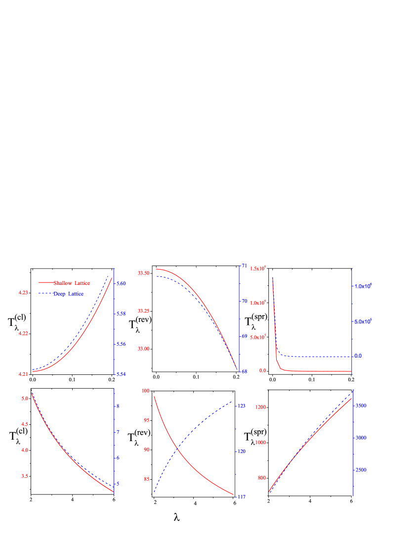
Figure 1: Left panel: Classical time period versus $\lambda$ for weak external modulation (a) and for strong external modulation (b). In this figure, for deep lattice $V_{0}=16E_{r}$, for shallow lattice $V_{0}=2E_{r}$ and $k^{-}=0.5$. Middle panel: Quantum revival time versus $\lambda$ for weak external modulation (c) and for strong external modulation (d). Right panel: Super revival time versus $\lambda$ when external modulation is weak (e) and for strong external modulation (f).

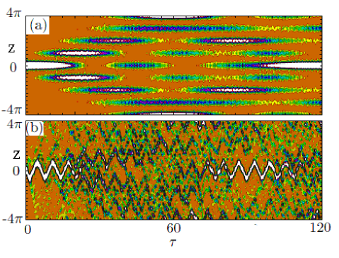
Figure 2: Spatiotemporal dynamics of atomic wave packet in the absence of modulation (a), and in the presence of modulation (b). The amplitude of modulation is $\lambda=3$ and $q=85.14$. Other parameters are $\tilde{V}_{0}=0.36$, $\Delta p=0.1$ and $k^{-}=0.16$.

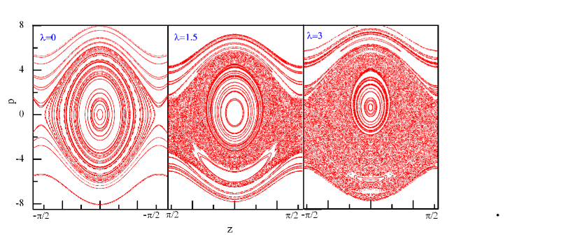
Figure 3: Poincaré phase space for driven optical lattice for modulation strengths $\lambda=0,1.5,3$ and potential depth $V_{0}=16E_{r}$

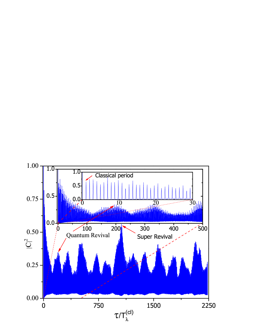
Figure 4: Square of auto-correlation function of a Gaussian wave packet is plotted versus time. Here, the parametric values are $\lambda=1.5$, $k^{-}=0.5$, $V_{0}=16E_{r}$, $\Delta z=\Delta p=0.5$. The wave packet is initially well localized at the central lattice well around the second band of undriven lattice. Classical period, revival time and super revival time are seen and indicated by arrows.

References

- (1) P. Bocchieri, A. Loinger, Phys. Rev. 107, 337 (1957).
- (2) F. Saif, Phys. Rep. 419, 207 (2005); ibid 425, 369 (2006).
- (3) R. Blumel, W. P. Reinhardt, Chaos in Atomic Physics (Cambridge university press, Cambridge, U.K. 2001).
- (4) F. Saif Phys. Rev. E 62, 6308 (2000).
- (5) F. Saif, J. Opt B: Quant. Semiclass. Opt. 7, S116 (2005).
- (6) S. I. Chu, D. A. Telnov, Phys. Rep. 390, 1 (2004).
- (7) R. Luter, L. E. Reichl, Phys. Rev. A 66, 053612 (2002); G. Hur et al, Phys. Rev. A 72, 013403 (2005); S. Fishman et al, Phys. Rev. Lett. 49, 509 (1982); X. Luo et al, 2008 Phys. Rev. A 77 053601; ibid 80, 053603 (2009); K. Hijii, S. Miyashita, Phys. Rev. A 81, 013403 (2010).
- (8) Vela-Arevalo Lu V, Fox R. F., Phys. Rev. A 71, 063403 (2005).
- (9) Hur G. et al, Phys. Rev. A 72, 013403 (2005).
- (10) Zhang C et al, Phys. Rev. B 73, 085307 (2006).
- (11) Villas-Bˆoas J M et al, Phys. Rev. B 70, 041302 (2004).
- (12) S. K. Son, S. I. Chu, Phys. Rev. A 77, 063406 (2008).
- (13) A. Eckardt et al, Phys. Rev. Lett. 95, 260404 (2005).
- (14) M. Holthaus, Phys. Rev. A 64, 011601 (2001).
- (15) W. K. Hensinger et al, Phys. Rev. A 70, 013408 (2004).
- (16) F. Saif, M. Fortunato, Phys. Rev. A 65, 013401 (2001).
- (17) S. Iqbal et al, Phys. Lett. A 356, 231 (2006).
- (18) J. M. Zhang, W. M. Liu, Phys. Rev. A 82, 025602 (2010); C. Petr et al, Phys. Rev. E 81, 046219 (2010); M. Heimsoth et al, Phys. Rev. A 82, 023607 (2010); A. Kenfack et al, Phys. Rev. Lett. 100, 044104 (2008); G. Lu et al, Phys. Rev. A 83, 013407 (2011); C. Sias et al, Phys. Rev. Lett. 100, 040404 (2008); C. Weiss, H. P. Breuer, Phys. Rev. A 79, 023608 (2009); C. Weiss, N. Teichmann, J. Phys. B 42, 031001 (2009); M. Roghani et al, Phys. Rev. Lett. 106, 40502 (2011).
- (19) K. W. Murch et al, Nat. Phys. 4, 561 (2008); K. Zhang et al, Phys. Rev. A 81, 013802 (2010); T. P. Purdy et al, Phys. Rev. Lett. 105, 133602 (2010); M. Paternost et al, Phys. Rev. Lett. 104, 243602 (2010); W. Chen et al, Phys. Rev. A 81, 053833 (2010); A. B. Bhattacherjee, Phys. Rev. A 80, 043607 (2009); J. Stettenheim et al, Nature 466, 86 (2010).
- (20) S Pötting et al, Phys. Rev. A 64, 023604 (2001).
- (21) P. J. Bardroff et al, Phys. Rev. Lett. 74, 3959 (1995).
- (22) M. G. Raizen, Adv. At. Mol. Opt. Phys. 41, 43 (1999).
- (23) F. Lenz et al, Phys Rev. E 82, 016206 (2010); ibd New J. Phys. 11 083035 (2009); W. Acevedo, T. Dittrich, J. Phys. A: Math. Theor. 42, 045102 (2009).
- (24) A. J. Lichtenberg, M. A. Liberman, Regular and Stochastic Motion, (Springer, Berlin, 1992).
- (25) L. E. Reichl, The Transition to Chaos, 2nd edition, (Springer, New York, 2004).
- (26) E. Ott, Chaos in dynamical systems 2nd edition (Cambridge University Press, Cambridge, 1993).
- (27) G. Qu´em´ener, John L. Bohn, Phys. Rev. A 83, 012705 (2011).
- (28) T. Gilbert et al, J. Phys. A: Math. Theor. 44, 065001 (2011); D. F. M. Oliveira et al, Physica D 240, 389 (2011).
- (29) M. E. Flatté, M. Holthaus, Ann. Phys. (N. Y.) 245, 113 (1996).
- (30) M. V. Berry, Philos. Tran. R. Soc. Lond. B 287, 237 (1997).
- (31) A. M. O. de Almeida, J. Phys. Chem. 88, 6139 (1984).
- (32) F. Saif, Eur. Phys. J. D 39, 87 (2006).
- (33) M. Abramowitz, I. A. Stegun, (eds.) The Handbook of Mathematical Functions (Dover, New York, 1970).
- (34) N. W. McLachlan, Theory and Applications of Mathieu Functions, (Oxford university press, London, 1947).
- (35) H. P. Breuer, M. Holthaus, Ann. Phys. 211, 249 (1991).
- (36) M. Born, Mechanics of Atoms, (Ungar, New Yark, 1960).
- (37) G. P. Berman, G. M. Zaslavsky, Phys. Lett. A 61, 295 (1977).
- (38) Y. I. Yukalov, Laser Phys. 19, 1 (2009).
- (39) F. L. Moore, et al, Phys. Rev. Lett. 73, 2974 (1994).
- (40) A. Eckardt et al, Phys. Rev. A 79, 013611 (2009); S. Arlinghaus, M. Holthaus, Phys. Rev. A 81, 063612 (2010); S. Arlinghaus, M. Langemeyer, M. Holthaus, in Dynamical Tunneling - Theory and Experiment, (Taylor & Francis, 2010).
- (41) S. Dryting, G. J. Milburn, Phys. Rev. A 47, 2484 (1993).
- (42) M. Ayub et al, J. Rus. Laser Res. 30, 205 (2009).
- (43) K. Drese, M. Holthaus, Chem. Phys. 217, 201 (1997).
- (44) M. Ayub, F. Saif, To be submitted.
- (45) A. M. Rey et al, Phys. Rev. A 72, 033616 (2005).
- (46) M. B. Dahan et al, Phys. Rev. Lett. 76, 4508 (1996).