Zero-Temperature Relaxation of Three-Dimensional Ising Ferromagnets

Abstract

We investigate the properties of the Ising-Glauber model on a periodic cubic lattice of linear dimension $L$ after a quench to zero temperature. The resulting evolution is extremely slow, with long periods of wandering on constant energy plateaux, punctuated by occasional energy-decreasing spin-flip events. The characteristic time scale $\tau$ for this relaxation grows exponentially with the system size; we provide a heuristic and numerical evidence that $\tau\sim\exp(L^{2})$. For all but the smallest-size systems, the long-time state is almost never static. Instead the system contains a small number of “blinker” spins that continue to flip forever with no energy cost. Thus the system wanders ad infinitum on a connected set of equal-energy blinker states. These states are composed of two topologically complex interwoven domains of opposite phases. The average genus $g_{L}$ of the domains scales as $L^{\gamma}$, with $\gamma\approx 1.7$; thus domains typically have many holes, leading to a “plumber’s nightmare” geometry.

I Introduction

We study the evolution of the homogeneous Ising ferromagnet on a periodic cubic lattice in which the spins are endowed with zero-temperature Glauber dynamics. Starting from an initial state of zero magnetization, corresponding to a supercritical temperature, conventional wisdom states that the spins organize into a coarsening domain mosaic whose characteristic length scale grows as $t^{1/2}$ GSS83 ; B94 ; GGGK ; book . This coarsening continues as long as the typical domain size is less than the linear dimension of the system $L$. At longer times, it is natural to anticipate that one of the ground states, with magnetization $m=+1$ or $m=-1$, should ultimately be reached.

For the one-dimensional system, this expectation is fulfilled — the ground state is always reached, independent of the initial condition. As one might expect by the diffusive dynamics of the spin domain interfaces, the characteristic time to reach this final state scales as $L^{2}$. In two dimensions, the ground state is no longer the only asymptotic outcome. A system that starts at zero magnetization may also get stuck in an infinitely long-lived metastable state that consists of straight single-phase stripes SKR01 ; SKR02 ; SS ; ONSS06 . The probability to reach such a stripe state was found numerically to be close to $\frac{1}{3}$. Recently, a theoretical argument was given BKR09 that relates the stripe state probability to certain exactly-calculated percolation crossing probabilities. The resulting probabilities to reach the stripe state are $\frac{1}{2}-\frac{\sqrt{3}}{2\pi}\ln\frac{27}{16}=0.3558\ldots$ for free boundary conditions and $0.3390\ldots$ for periodic boundary conditions, in agreement with simulation data SKR01 ; SKR02 .

For regular lattices in three dimensions or greater, little is known about the evolution and long-time state of this kinetic Ising ferromagnet. If the initial magnetization is non-zero, it is generally believed that this system (on an even-coordinated lattice in $d\geq 2$) ultimately reaches the ground state of the majority phase in the thermodynamic limit, no matter how small the initial magnetization M10 . This result has not been proved, even in two dimensions, although it is plausible because of the connection with percolation BKR09 . In the $d\to\infty$ limit, the fact that the (majority) ground state is reached is intuitively obvious and has been recently proved in Ref. M10 . Physically, however, the zero initial-magnetization state is much more important than the general case of a non-zero magnetization. Indeed, the usual coarsening process begins at a temperature that exceeds the critical temperature where the initial magnetization (of an infinite system) equals zero. We therefore focus on the case of zero initial magnetization in this paper.

An earlier study SKR02 found that an $L\times L\times L$ Ising ferromagnet on a cubic lattice exhibits a much more complex evolution than the corresponding two-dimensional system. In particular, the long-time state is typically topologically complex and not static. Here, we investigate the three-dimensional system in greater detail OKR11 . We offer new perspectives to help understand the long-time state of the system and present simulation results to quantify its unusual properties.

While the ground state is a possible long-time outcome of the dynamics, it happens that a geometrically rich and infinitely long-lived metastable state (Fig. 1) arises with overwhelming probability. This long-time state typically has a sponge-like geometry, with multiple interpenetrating regions of positive and negative magnetization. The continuum version of this state is one in which the mean curvature of the interface is zero. This restriction leads to a veritable zoo of possible geometries that have been extensively cataloged S90 ; S69 . A few illustrative examples of a subclass of these systems — periodic zero-curvature continuum interfaces — are given in Fig. 2. These structures also resemble the geometrically complex arrangements that arise in two-phase micellar systems, and are popularly known as “plumber’s nightmares” L89 ; AS89 ; FUTGW ; AECTB .

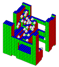
Figure 1: (color online) A typical example of a state with blinker spins for a $20^{3}$ cubic lattice with periodic boundary conditions. The highlighted blocks indicate blinker spins.

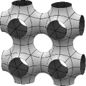
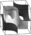
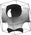
Figure 2: Triply-periodic minimal surfaces in three dimensions. Figures provided by K. Brakke (see also Ref. AECTB ).

Intriguingly, the long-time state of the three-dimensional system is generally not static, but rather, contains stochastic blinker spins that can flip repeatedly without any energy cost. The interfaces defined by these spins can therefore wander ad infinitum on a connected but bounded set of equal-energy blinker states as illustrated in Fig. 1. Here the cubes correspond to up spins (with the spin at the cube center), while the down spins correspond to blank space. The highlighted cubes indicate spins at the convex (outer) corners of domain interfaces that can flip with no energy cost. There are also oppositely-oriented spins (blank spaces) adjacent to the apex of the concave corners that can also flip up with no energy cost. A blinker state wanders perpetually on a small set of iso-energy points in state space. Blinker states first appear (albeit rarely) when the linear dimension $L=5$, but essentially all configurations contain blinkers for large $L$. While the fraction of blinker spins is quite small, the fraction of the system volume over which blinker spins can wander is macroscopic — it is usually of the order of ten percent for large $L$.

In Sect. II, we define the system under study. In Sect. III, we present a simple method to accelerate the simulations. Details about the accuracy of this acceleration algorithm are given in Appendix A. We then discuss the physical properties of the long-time state of the system in Sect. IV, including details about blinker states (Sect. IV.1), the asymptotic energy of the system (Sect. IV.2), and topological characteristics of the domains (Sect. IV.3). Additional facts about the $L$-dependence of some basic observables are given in Appendix B. Typically, domain interfaces have large genus so that the domains have many interpenetrating protrusions. Finally, we investigate the time dependence of the survival probability (Sect. IV.4), namely, the probability that the energy of the system is still decreasing up to a given time. Based on the insights gained from studying blinker states, we can understand some important features of this survival probability. Concluding remarks are given in Sect. V. Basic features of the evolution of a $2^{3}$ system, where all states can be enumerated exactly, as well as a few details of slightly larger systems are are presented in Appendix B.

II Model

The Hamiltonian of the ferromagnetic Ising model is

$$\mathcal{H}=-\sum_{\langle ij\rangle}\sigma_{i}\sigma_{j}\,,$$ (1)

where $\sigma_{i}=\pm 1$ denotes the spin at site $i$, the interaction strength is set to one, and the sum is over all nearest-neighbor pairs of sites. If not stated explicitly otherwise, we consider the cubic lattice of linear dimension $L$, with $L$ even, and with periodic boundary conditions. There are two natural choices for the initial state: (i) initially uncorrelated and equal fractions of $+1$ and $-1$ spins (corresponding to an initial temperature $T=\infty$), or (ii) the antiferromagnetic initial condition, in which all pairs of neighboring spins are oppositely oriented. The long-time evolutions of the system starting from these two initial states are similar, with only small quantitative differences in the distribution of basic physical observables, such as the energy and magnetization in the long-time state. Thus we focus on the antiferromagnetic initial state for concreteness and for simplicity.

The spins evolve by zero-temperature single spin-flip Glauber dynamics glauber . To implement this dynamics at zero temperature, we keep a list of flippable spins — those where the energy change of the system $\Delta E$ would be zero or negative if the spin were to flip. (At zero temperature, spin-flips which would lead to an increase of energy, $\Delta E>0$, are forbidden book .)  By picking only the spins from this list, we eliminate the time that would be wasted in picking and simulating non-flippable spins. In each update, we pick a flippable spin at random and flip it with probability 1 if $\Delta E<0$, or with probability $\tfrac{1}{2}$ if $\Delta E=0$. This update corresponds to majority rule, as the condition $\Delta E<0$ means that the majority of neighbors are antiparallel to the selected spin.

More generally, zero-temperature single spin-flip dynamics is defined by the rules,

$$\text{Flipping probability}=\begin{cases}1&\text{if}\quad\Delta E<0,\\ p&\text{if}\quad\Delta E=0,\\ 0&\text{if}\quad\Delta E>0,\end{cases}$$ (2)

that depend on the single parameter $p$. For the heat-bath and Glauber dynamics, $p=\tfrac{1}{2}$, while for the Metropolis algorithm Metropolis all updates proceed with the same rate ($p=1$). While the behavior for all $p>0$ is essentially independent of $p$, the $p=0$ case is special, as the system quickly gets trapped in a jammed configuration Luck . We shall avoid the $p=0$ dynamics with only strictly energy-lowering spin flips, as this case is relevant for a special class of kinetically constrained systems (see KC for review). Since the choice for the parameter $p$ is arbitrary (as long as $p$ is strictly positive), we fix $p=\tfrac{1}{2}$, although this choice is essentially a matter of habit and, e.g., the Metropolis algorithm with $p=1$ is more efficient.

For the antiferromagnetic initial condition, all spins are initially flippable. The number of flippable spins decreases rapidly at early times and then the decrease slows down as the system coarsens. After each update event, the time is incremented by 1/#(flippable spins). Thus in one time unit, each flippable spin changes its state once on average. This update step is applied repeatedly and the dynamics is averaged over many realizations to determine the evolution of the system.

III Acceleration Algorithm

The evolution of the system becomes so slow that the standard Glauber dynamics algorithm described above is inadequate to probe the long-time properties of even reasonably-sized systems. Figure 3 illustrates this slowing down for the energy evolution of a typical realization of a $20^{3}$ system. The main panel shows the time dependence of the gap between the actual energy and the ground state energy divided by the total number of spins. Henceforth, we term this normalized difference as the “energy” $E_{L}$. For this example, the data are roughly consistent with the $E_{L}\sim t^{-1/2}$ for $1\lesssim t\lesssim 10^{2}$.

Figure 3: Time dependence of the energy for a representative realization of a $20^{3}$ system whose energy stops evolving at $t\approx 41712$. The inset shows the long-time tail of the same data; note that the abscissa is $\ln t$.

For times beyond the coarsening time (which scales as $L^{2}$), the energy evolution is characterized by long periods where only zero-energy spins can flip (those with equal numbers of up and down neighbors). These long periods of stasis are punctuated by progressively more rare energy-decreasing events (inset to Fig. 3). Thus the system typically wanders on successive plateaux that define a set of iso-energy points in state space. Occasionally there is a drop to a lower plateau by an energy-lowering spin-flip event (Fig. 4). This feature is illustrated in Fig. 5, where we plot the configuration averaged time $\Delta t_{n}$ between successive energy-lowering spin-flip events as a function of $t_{n}$, the average time at which the $n^{\rm th}$ such event occurred. Over a substantial range, $\Delta t_{n}$ appears to grow exponentially with $t_{n}$, so that most of the evolution is spent wandering aimlessly on iso-energy plateaux. A somewhat related continuum picture of this state space evolution is presented in Refs. KL96 ; F97 .

Figure 4: Schematic illustration of the state of the system wandering on fixed-energy plateaux at long times.

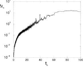
Figure 5: Average time $\Delta t_{n}$ between successive energy-lowering spin-flip events as a function of $t_{n}$, the time for the $n^{\rm th}$ such event for $1024$ realizations of a $10\times 10\times 10$ system. The data are smoothed over a 100-point range.

To reduce the time spent in simulating these iso-energy wanderings, we constructed an acceleration algorithm and tested that the long-time state achieved by this algorithm is virtually identical to that of the true zero-temperature Glauber dynamics. Our method is based on imposing a weak field while the system is on any single iso-energy plateau to reduce the time needed to find the next energy lowering event. The field is reversed after each such event so that the average field is zero. The steps of our method are the following:

• Apply Glauber dynamics (to flippable spins only) until $t=5L^{2}$. This time is sufficiently beyond the coarsening time that energy-lowering events have become rare (Fig. 3).

• For $t>5L^{2}$, apply an infinitesimal field to drive the state-space motion along a fixed-energy plateau. Thus the next energy-lowering event (if it exists) is found more rapidly than if no field was applied.

• After each energy-lowering event occurs, the sign of the field is reversed, leading to the alternating state-space motion sketched in Fig. 4.

• If the number of active spins goes to zero without a drop in energy while the field is applied, the field is reversed. From this configuration, the system evolves by zero-temperature Glauber dynamics with the reversed field. If the number of active spins again goes to zero without a drop in energy, then the final energy value has been reached and the simulation is finished.

We verified that this acceleration algorithm accurately reproduces the energy obtained by straightforward Glauber dynamics for $L\leq 10$, where a direct check of this acceleration method is computationally feasible. For this check, we take all configurations that have been evolved to $t=5L^{2}$ by zero-temperature Glauber dynamics and evolve each one both by continuing the Glauber dynamics and by our acceleration algorithm until no flippable spins remain. Over $10^{7}$ realizations the fractional difference between the energies obtained by these two methods is $\leq 1.4\times 10^{-8}$. Moreover, the distributions of the final energies are virtually indistinguishable.

For larger $L$, time to reach the final energy by zero-temperature Glauber dynamics is too long to amass sufficient statistics. Instead, we compare the ultimate energy that is reached by starting the acceleration algorithm at progressively later times. As shown in the Table 1 in Appendix A, the energy that is ultimately reached changes by a negligible amount as the cutoff time is increased. For example, for $L=100$, the error in the final energy reached by the acceleration algorithm is of the order of $5\times 10^{-5}$. Moreover, as illustrated in this table, the acceleration algorithm is considerably faster than the zero-temperature Glauber dynamics. Thus we use the acceleration algorithm for all of our simulation results. On a 32-core machine, we are able to simulate $10^{5}$ realizations of a $90^{3}$ system in approximately ten days of running time.

IV The Long-Time State

At sufficiently long times, the energy of each realization stops decreasing, either because a blinker configuration is reached or occasionally a static final state is reached. Figure 6 shows that the probability of reaching a blinker configuration approaches 1 as $L\to\infty$. This observation is one of our main results, for which preliminary corroboration was given earlier SKR01 ; SKR02 . Somewhat surprisingly, for the initial condition where the magnetization is zero but with otherwise uncorrelated spins, the probability to reach a stationary state vanishes more rapidly in the $L\to\infty$ limit than for the antiferromagnetic initial condition. Even though a blinker consists of a set of states of the same energy, we term the “final state” these constant-energy configuration(s) that are reached when the energy stops decreasing.

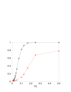
Figure 6: Plot of $1-P_{b}$, the complement of the probability $P_{b}$ of reaching a blinker configuration ($\circ$), and $1-P_{2}$, the complement of the probability $P_{2}$ of reaching a state that consists of 2 clusters ($\bigtriangleup$), as a function of $1/L$.

In this final state, the spins almost always partition into two and only two interpenetrating clusters. Using the Hoshen-Kopelman cluster-multilabeling algorithm HK76 to determine the distribution of the number of clusters, we find that the probability to find a single cluster (corresponding to the ground state) or more than two clusters in the final state rapidly decays with $L$ (Fig. 6). Final states that contain more than two clusters typically consist of multiple narrow filaments of one phase in a surrounding background of the opposite phase. In all of our simulations on the $L\times L\times L$ cubes with periodic boundary conditions, the largest number of clusters observed in any realization was seven. (This happened to occur in a $38^{3}$ system, where the realization consisted of six narrow filaments of one phase in a background of the opposite phase.)

IV.1 Relaxation of Blinker Configurations

As we now discuss, blinker states are responsible for the very slow relaxation of the spin system at long times. To appreciate the underlying mechanism, it is instructive to study the dynamics of the synthetic blinker states shown in Fig. 7. In this example, the domain of up spins consists of three orthogonal $4\times 12$ slabs, each of which wraps periodically, so that the apparent slab corners are merely visual artifacts. In the cavity defined by the confluence of the three slabs, a blinker state exists. By zero-energy spin flips, the portion of the interface defined by this cavity can be in the extremes of fully deflated (left panel of Fig. 7), or fully inflated (right), or in some intermediate state (middle). Note that each extreme configuration possesses a single blinker spin, while intermediate configurations have more than one blinker spin. Although each blinker spin does not experience any energetic bias, there is an effective geometric bias that drives the interface to the half-inflated state. This effective bias is controlled by the difference in the number of flippable spins on the convex and concave corners on the interface, $N_{+}$ and $N_{-}$, respectively. When the cube is mostly inflated $N_{+}-N_{-}$ is positive so that the interface tends to deflate, and vice versa when the cube is mostly deflated. Thus the effective bias drives the interface to the half-inflated state.

We quantify the evolution of this synthetic blinker by the average first-passage time $\langle t\rangle$ for an $\ell\times\ell\times\ell$ fully-deflated blinker to become fully inflated. To estimate this time, it is helpful to first consider the corresponding two-dimensional system (Fig. 8). Near the half-inflated state, the interface consists of $N_{+}$ outer corners and $N_{-}$ inner corners, with $N_{+}-N_{-}=1$ in two dimensions and $N_{+}\sim\ell$. In a single time unit, all eligible spins on the interface flip once, on average. Since $N_{+}-N_{-}=1$, the interface area typically decreases by 1. Thus we infer an interface velocity $u=\Delta A/\Delta t\sim-1$. Similarly, the mean-square change in the interface area is of the order of $N_{+}\sim\ell\sim\sqrt{A}$. Thus the effective diffusion coefficient $D$ is proportional to $\ell$. The first-passage time is dominated by the time to move from the half-inflated state to the fully-inflated state by flipping of the order of $A=\ell^{2}$ spins. Since this process is moving against the effective bias, the dominant Arrhenius factor fpp in the first-passage time is $\tau\sim\exp(|u|\ell^{2}/D)$, so that

$$\ln\tau\sim\ell\,.$$ (3)

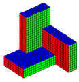
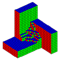
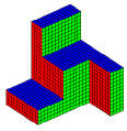
Figure 7: (color online) An $8^{3}$ blinker on a $20^{3}$ cubic lattice, showing the fully-deflated state (left), an intermediate state (middle), and the fully-inflated state (right). The bounding slabs wrap periodically in the three Cartesian directions.

Figure 8: Two-dimensional analog of the blinker states in Fig. 7.

For the corresponding three-dimensional system of volume $V=\ell^{3}$, there are typically $N_{\pm}\sim\ell^{2}$ outer and inner corners when the interface is half inflated. The disparity in their number is now of the order of $\ell$. Thus in a single time step the displacement of the interface is of the order of $\ell$; this quantity coincides with the interface velocity. Similarly, the mean-square change in the interface volume in a unit time, which coincides with the diffusivity, is of the order of $N_{\pm}\sim\ell^{2}\sim D$. Consequently, the leading behavior of the first-passage time is

$$\ln\tau\sim u\ell^{3}/D\sim\ell^{2}\,.$$ (4)

The direct generalization of this argument to $d$ dimensions gives $\ln\tau\sim\ell^{d-1}$. Related aspects of slow evolution in three dimensions were discussed for the homogeneous kinetic Ising ferromagnet L99 and for a kinetic Ising system with competing ferromagnetic and antiferromagnetic interactions SHS .

Figure 9 shows simulation data for the first-passage time from the fully-deflated to the fully-inflated state in two and three dimensions. The agreement between Eq. (3) and the two-dimensional data is excellent. In three dimensions, simulations are necessarily limited to very small $\ell$, while our crude argument is asymptotic; nevertheless, the data are qualitatively consistent with Eq. (4). The salient result is that the time for a fully-deflated blinker to become fully inflated grows rapidly with $\ell$.

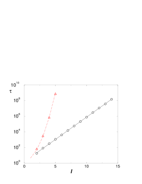
Figure 9: First-passage time from the fully-deflated to the fully-inflated state for $d=2$ ($\circ$) and $d=3$ ($\bigtriangleup$). The line for $d=2$ is the best fit $\tau=1.40\,\exp(1.33\,\ell)$, while the curve for $d=3$, $\tau=3\,\exp(0.8\,\ell^{2})$, is merely a guide for the eye. Each data point is based on at least 128 realizations.

From the dynamics of the synthetic blinker of Fig. 7, we can now understand the long time scales associated with the relaxation of a large system. Indeed, consider two such blinkers that are oppositely oriented and spatially separated so that they do not overlap when both are half inflated, but just touch corner to corner when both are inflated (Fig. 10). As long as the blinkers do not overlap, their fluctuations do not change the energy of the system. However, if these blinkers touch, then a spin flip event has occurred that lowers the energy. After this irreversible coalescence, subsequent spin flip events cause the two blinkers to ultimately merge.

Figure 10: A schematic two-dimensional projection of a blinker coalescence event. The tips of the blinkers correspond to the fully-inflated configuration shown in the right panel of Fig. 7.

Because of the impermanence of a two-blinker configuration, we term it a pseudo-blinker. We assert that each coalescence of a pseudo-blinker corresponds to one of the increasingly rare energy-lowering spin-flip events sketched in Fig. 4. The time for pseudo-blinker coalescence is extraordinarily long because the time for each blinker to reach a nearly-inflated state is a rapidly increasing function of its size. These coalescences correspond to energy-lowering spin-flip events at long times.

We now turn to the true blinker states. As might be anticipated from the example in Fig. 1, simulations indicate that the fraction of blinker spins is small — of the order $3\times 10^{-3}$ to $4\times 10^{-3}$ of all spins for systems of linear dimension $L\leq 50$. The instantaneous number of blinker spins also fluctuates substantially so that their number is not a meaningful characteristic of the blinker states. A more robust measure is the total volume that is accessed by blinker spins. We determine this accessible volume as follows: Once a true blinker state is first reached (which we define as $\mathcal{B}_{0}$), we drive the system with an infinitesimal positive field until the spin configuration $\mathcal{B}_{+}$, with no flippable spins, is reached. Then starting again from $\mathcal{B}_{0}$, we drive the system with an infinitesimal negative field until there are no flippable spins and the configuration $\mathcal{B}_{-}$ is reached. The difference $|\mathcal{B}_{+}-\mathcal{B}_{-}|$ defines the total blinker volume. The resulting blinker volume fraction is a slowly increasing function of $L$ and extrapolating to $L\to\infty$ gives an asymptotic blinker volume fraction of approximately 9% — a finite fraction of the entire system.

IV.2 Asymptotic Energy

An important characteristic of a finite system of linear dimension $L$ is its energy $E_{L}$ at infinite time. As mentioned in Sect. III, what we term the energy is actually the energy gap above the ground state energy per spin. This energy decreases with $L$ in a manner consistent with the power-law dependence ${E}_{L}\sim L^{-\epsilon}$ (Fig. 11). However, there is systematic curvature in this data, and we extrapolate the local two-point slopes in the plot of $E_{L}$ versus $L$ to obtain the estimate $\epsilon\approx 1$, in agreement with previous results based on smaller-scale simulations SKR02 . This dependence implies that the total interface area between spin domains scales as $L^{2}$.

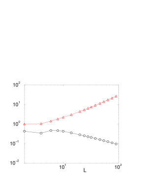
Figure 11: Normalized average energy $(\circ)$ and genus of the final state ($\bigtriangleup$) as a function of $L$. The relative error for each data point is less than $1.4\times 10^{-3}$.

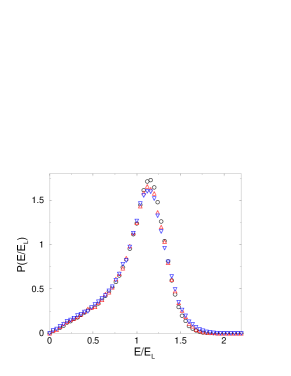
Figure 12: The normalized final-state energy distribution for $L=54$ ($\circ$), $L=76$, ($\bigtriangleup$), and $L=90$ ($\bigtriangledown$).

The scaled distribution of energies, $P(E/E_{L})$, exhibits an excellent data collapse (Fig. 12). The distribution has a well-defined peak that is close to a Gaussian; there is also a noticeable linear tail at low energies. The fact that the energy distribution $P(E/E_{L})$ remains broad in the thermodynamic limit is not surprising as all our numerical findings show the lack of self-averaging. It would be interesting to understand qualitatively the shape of the energy distribution $P(E/E_{L})$, or at least the asymptotic behaviors in the $E/E_{L}\to 0$ and $E/E_{L}\to\infty$ limits.

IV.3 Domain Topology

The long-time state of the three-dimensional system is, in general, topologically complex because it is possible — in fact likely — that the interface contains many holes 2d . The number of holes is also known as the genus $g$. Formally, the genus of a connected, orientable surface is an integer that represents the maximum number of cuts that can be made through the surface along non-intersecting closed simple curves without disconnecting the resulting manifold. As elementary examples, the genus of a sphere is $g=0$, while the genus of a doughnut is $g=1$.

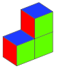
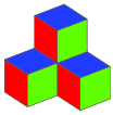
Figure 13: (color online) Simple examples of interfaces with genus $g=2$ and $g=3$ for a periodic $2\times 2\times 2$ system.

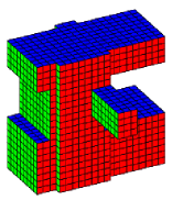
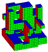
Figure 14: (color online) Examples of a low-genus ($g=3$) and high-genus ($g=16$) domain on a $20^{3}$ lattice.

The genus of a surface can be expressed through its Euler characteristic $\chi$ (see e.g. E ; Japan )

$$\chi=2(1-g)=\mathcal{V}-\mathcal{E}+\mathcal{F}.$$ (5)

The latter equality relates the Euler characteristic to easily-measured features of the domain interface: $\mathcal{V}$, the number of vertices on the interface, $\mathcal{E}$, the number of edges, and $\mathcal{F}$, the number of faces. As simple examples, the Euler characteristic of an isolated cube is $\chi=8-12+6=2$, corresponding to genus 0. (Topologically, the cube is identical to the ball, so the boundary of the cube is a sphere.)  The Euler characteristic of a linear filament that wraps around the torus in one direction is zero. By discretizing this filament as a $2\times 1$ cluster that wraps onto itself, we have $\mathcal{V}=8$, $\mathcal{E}=16$ and $\mathcal{F}=8$, corresponding to genus $g=1$. Note that the Euler characteristic does not depend on the length scale of the discretization. Similarly for a cluster that percolates in two directions (Fig. 13), $\chi=8-20+10=-2$ so the genus $g=2$. Finally for a cluster that percolates in all three Cartesian directions, $\chi=8-24+12=-4$ so the genus $g=3$.

Since blinker spins do not affect the topology, we freeze these spins in their orientations at the time when the interface topology is measured. To measure the topology, we first identify all the clusters in the final state by the Hoshen-Kopelman algorithm HK76 . We then compute the Euler characteristic of each cluster. If there are only two clusters, then by construction they have the same interface and thus the same Euler characteristic. If a final state has more than two clusters, we use the maximum genus among all clusters as the genus of the system. To determine the Euler characteristic numerically, we first determine the number of faces $\mathcal{F}$. This quantity equals the number of neighboring antiparallel spins (accounting for the periodic boundary conditions) which, in turn, is directly related to the energy of the system. Once we identify a new face on the interface, each of the four vertices and the four edges bounding this face are added to the current counts of $\mathcal{V}$ and $\mathcal{E}$, as long as they have not yet already been counted as part of another previously-encountered face.

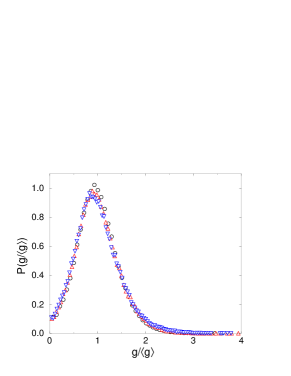
Figure 15: The final-state genus distribution for $L=54$ ($\circ$), $L=76$, ($\bigtriangleup$), and $L=90$ ($\bigtriangledown$).

The resulting domain topologies are quite diverse (Fig. 14). For example, for $L=20$, the smallest genus observed was 1, the largest genus was 18, while the average genus is approximately 4.36. The average genus for a given $L$, defined as $g_{L}$, again appears to grow as a power law in $L$, $g_{L}\sim L^{\gamma}$, but with substantial finite-size corrections (Fig. 11). Analogous to the behavior for the average energy, the data for $g_{L}$ versus $L$ on a double logarithmic scale are systematically curved upward and extrapolating the effective exponent to $L\to\infty$ yields the estimate $\gamma\approx 1.7$. The scaled genus distributions at long times for $L=54$, $76$, and $90$ also show excellent data collapse (Fig. 15).

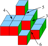
Figure 16: A portion of an interface to illustrate vertices (labelled) that are shared among 3, 4, 5, or 6 edges.

Although we separately studied the energy and the genus, these two quantities can be intimately connected by simple topological considerations. We start by simplifying Eq. (5). For a closed surface that defines the interface between spin domains, each face has 4 edges and each edge must be shared between 2 adjacent faces. Hence

$$\mathcal{E}=2\mathcal{F}.$$ (6)

Similarly, each edge has 2 vertices and each vertex is shared among 3, 4, 5, or 6 adjacent edges (Fig. 16). This leads to the bounds

$$\frac{\mathcal{E}}{3}\leq\mathcal{V}\leq\frac{2\mathcal{E}}{3}~{}.$$ (7)

Using these two relations in Eq. (5) gives

$$-\frac{\mathcal{F}}{3}\leq\chi\leq\frac{\mathcal{F}}{3}~{}.$$ (8)

While the lower bound is useful, the upper bound can be replaced by the much stronger condition $\chi\leq 2$, with the maximal value of 2 being achieved for a sphere. With this replacement, we obtain the following bounds on the genus:

$$0\leq g\leq\frac{\mathcal{F}}{6}+1.$$ (9)

However, $\mathcal{F}$ is directly related to the total energy of the system because each face corresponds to a single pair of anti-aligned spins per spin and thus has an energy cost of $+2$ (when the interaction strength is set to 1, see Eq. (1)). Thus $\mathcal{F}=L^{3}E_{L}$.

Finally, we make the guess that the actual value of $g$ lies roughly midway between the upper and lower bounds; namely, $g\propto\mathcal{F}$. Using our exponent definitions $E_{L}\sim L^{-\epsilon}$ and $\langle g\rangle\sim L^{\gamma}$, our argument leads to the exponent inequality

$$\epsilon+\gamma\leq 3.$$ (10)

Our numerical estimates for these two exponents given above, $\epsilon\approx 1$ and $\gamma\approx 1.7$ are consistent with Eq. (10).

We can carry this analysis a bit further by making use of some simple facts in discrete differential geometry GB . Let us define the number of vertices with $m$ incident edges as $\mathcal{V}_{m}$. It is useful to introduce the notion of a “defect” that is associated with each vertex. The defect for a vertex is defined as the difference between the sum of the angles of all the faces at the vertex and $2\pi$. With this definition, it is easy to see that the defect of a vertices of types 3, 4, 5, and 6 are $\frac{\pi}{2}$, 0, $-\frac{\pi}{2}$, and $-\pi$, respectively. For any domain, the total defect of all vertices on the surface equals $2\pi\,\chi$; this is essentially the Gauss-Bonnet theorem for a discrete interface GB . Thus we have the general relation (see Eq. (5))

$$\frac{\pi}{2}\,\mathcal{V}_{3}-\frac{\pi}{2}\,\mathcal{V}_{5}-\pi\,\mathcal{V}_{6}=2\pi\,\chi=4\pi(1-g).$$ (11)

Therefore the genus of a surface and the number of vertices of various types are related by

$$g=1+\frac{1}{8}(2\mathcal{V}_{6}+\mathcal{V}_{5}-\mathcal{V}_{3})\,.$$ (12)

From the examples of domains shown throughout this work, almost all vertices are of type $m=4$ while vertices of type $m=5$ seem to be next most common. Vertices of type $m=3$ are associated with blinkers and therefore should be few in number. Vertices of type $m=6$ arise at a 3-fold branch of the domain and therefore seem to be the most rare. Thus we expect that vertices of type $m=5$ scale the same way as $\langle g\rangle$ which numerically appears to grow as $L^{1.7}$.

IV.4 Survival Probability

The relaxation process is naturally characterized by $S(t)$, the probability that the energy of the system is still decreasing at time $t$. Since energy-lowering spin flips occur rarely at long times, it is not immediately evident whether the most recent energy-lowering spin flip is the last such event or whether another energy-lowering flip event will occur sometime in the distant future. To determine if the energy has reached its final value in an efficient way, we use the following algorithm that is a variant of our acceleration algorithm. As a preliminary, we separately track both positive-energy and zero-energy flippable spins; the former are those for which the energy decreases if such a spin actually flips. We start the simulation by running zero-temperature Glauber dynamics until no positive-energy flippable spins remain. At this time, defined as $T_{0}$, the configuration $\mathcal{C}_{0}$ may have reached the final value of the energy.

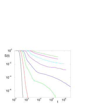
Figure 17: Survival probability $S(t)$ versus time $t$ for $L=4,6,8,10,14,20,30$ and $40$ (lower left to upper right) on a double logarithmic scale. The averaging has been performed over $10^{7}$ realizations for $L\leq 10$, $10240$ realizations for $L=14,20,30$, and 2048 realizations for $L=40$.

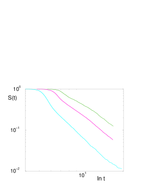
Figure 18: $S(t)$ versus $\ln t$ for $L=20,30,$ and 40 on a double logarithmic scale.

We now proceed as follows:

• Apply an infinitesimal magnetic field. If an energy-lowering spin-flip occurs, then the energy of $\mathcal{C}_{0}$ is not the final energy. In this case, the system is returned to $\mathcal{C}_{0}$ and subsequently evolves by Glauber dynamics until again no positive-energy spins remain and a new candidate final configuration and final time is reached.

• If an energy-lowering spin-flip does not occur, the system is returned to $\mathcal{C}_{0}$ and a field is applied in the opposite direction. Again, if an energy-lowering spin-flip occurs, the system is returned to $\mathcal{C}_{0}$ and subsequently evolves by Glauber dynamics until no positive-energy spins remain and a new candidate final state is reached.

• If an energy-lowering spin-flip does not occur after the field has been applied in both directions, then $\mathcal{C}_{0}$ is at the final energy and the survival time equals $T_{0}$.

We record the time when the energy of a system stops changing, from which we infer the time dependence of the survival probability $S(t)$. This time dependence is both surprisingly complex and extremely slow for small system sizes (Fig. 17). For example, for $L=10$, $40$ realizations had not yet relaxed to their ultimate energy by $t=10^{9}$, a time that is seven orders of magnitude beyond the coarsening time scale of $10^{2}$. The data cutoff for $L\geq 10$ was imposed because of CPU time limitations. By $L=20$, the dependence of $S(t)$ on $t$ becomes smooth and reasonably systematic and a plot of $S(t)$ versus $\ln t$ on double logarithmic scale (Fig. 18) suggests that the long-time data can be reasonably fit to an inverse logarithmic dependence $S(t)\sim(\ln t)^{-\sigma}$, with $\sigma\approx 3$.

V Discussion

We investigated the evolution of the kinetic Ising model that is endowed with single spin-flip dynamics on a finite cubic lattice with periodic boundary conditions. The system starts in the antiferromagnetic state and is quenched to zero temperature. The details of the initial conditions are secondary as long as the magnetization vanishes. (If the initial magnetization is non-zero, the evolution is much simpler and the Ising ferromagnet falls into a ground state.)  We asked the simple question: what happens? A natural expectation might be that the ground state should be reached. A more comprehensive version of this presumption is encapsulated by the central dogma of coarsening, which asserts:

1. Ising ferromagnets have just two metastable states, which coincide with the ground states.

2. If an Ising ferromagnet is endowed with zero-temperature single spin-flip dynamics, or more generally with a non order-parameter conserving dynamics, then one of the two ground states is necessarily reached.

3. The time to reach a ground state scales with the linear dimension of the system as $L^{2}$.

This central dogma is indeed correct in one dimension. However, for two-dimensional Ising ferromagnets, there are numerous metastable states that consist of single-phase stripes whose total number grows as $\mathcal{M}_{2}\sim g^{L}$ SKR01 , where $g=\tfrac{1}{2}(\sqrt{5}+1)$ is the golden ratio. Nevertheless, the failure of the central dogma in two dimensions is rather benign, as one of the ground states is reached SKR01 ; SKR02 ; BKR09 with probability close to 2/3. Moreover, for most realizations, the final state (either a ground state or a stripe state) is approached in a time that scales as $L^{2}$.

In three dimensions, however, the central dogma completely fails; viz., all its three basic tenets are wrong. First, the number of metastable states $\mathcal{M}_{3}$ scales exponentially with the system size: $\ln\mathcal{M}_{3}\sim L^{3}$ AP . Further, the ground states are never reached (for sufficiently large systems) and the relaxation time is anomalously long. We provided heuristic and numerical evidence that the relaxation time scales as $e^{L^{2}}$. Thus for a macroscopic system with $L\sim 10^{8}$ the relaxation time considerably exceeds any time scale in the Universe.

Since the approach to the long-time state is extraordinarily slow, even for a system as small as $10\times 10\times 10$, there are still realizations (albeit a small fraction) for which the energy has not yet reached its final value by $t=10^{9}$, whereas the standard coarsening time is of the order of $10^{2}$. We constructed a physical picture, based on the coalescence of blinker-like configurations, that instead predicts a relaxational time scale that grows exponentially in the linear dimension of the system. In particular, the survival probability $S(t)$, defined as the probability that the energy has not yet relaxed to its final value by time $t$ seems to decay as a power law in $1/\ln t$. While the mechanism of blinker coalescence appears plausible, we do not have a theoretical explanation for the functional form of $S(t)$. The primary feature of the relaxation that we wish to emphasize is that the standard picture of coarsening, characterized by a time that scales as $L^{2}$, is inappropriate for the three-dimensional Ising model with zero-temperature Glauber dynamics.

Another striking feature of the three-dimensional Ising ferromagnet is that a set of connected metastable microstates with equal energy is reached rather than a ‘frozen’ metastable state. Each such set of states contains a small number number of flippable blinker spins that can flip ad infinitum without any energy cost. Thus the system can wander within one of these iso-energy sets forever. Even though the number of blinker spins is small, the spatial volume over which the blinker spins can roam comprises of the order of 10% of the volume of system in the limit of large $L$.

The topology of the long-time state is much richer than that of the corresponding two-dimensional system. In two dimensions, the only possible states at infinite time are the ground state or an even number of alternating single-phase stripes (for periodic boundary conditions). In contrast, the long-time states in three dimensions are highly interpenetrating and contain many holes (Fig. 14). Correspondingly, the average genus of the domains scales with linear dimension as $L^{1.7}$. Aside from this global characterization of the domains, it is not clear what are the most useful measures of the domain geometry.

While we focused on the cubic lattice, similar behaviors should arise for the kinetic Ising model on other even-coordinated lattices in three dimensions. We deliberately avoided odd-coordinated lattices or other complex networks where the coordination can be odd, as the zero-temperature Ising-Glauber system quickly freezes, in disagreement with the central dogma predictions. However, this freezing has a local and trivial nature. For example, for an odd-coordinated lattice, single-phase droplets can arise, in which spins within a droplet each have more internal than external neighbors NS ; pontus ; dean ; CP06 ; H09 , as illustrated for the example of a hexagonal droplet on the hexagonal lattice (Fig. 19). These droplets can thus remain forever in the phase opposite to that of the background. Another example of this local freezing is the Ising model with zero-temperature Kawasaki (spin exchange) dynamics book , where again local defects quickly arise that stop the overall relaxation process.

Figure 19: Example of a frozen cluster of up spins on the hexagonal lattice.

Intriguing and mostly unexplored behaviors arise for non-cubic systems (Fig. 20), for example, a $L\times L\times aL$ system. When the aspect ratio $a$ is small, the system becomes a thin square slab. We are generically interested in the thermodynamic limit $L\to\infty$ with $a$ fixed, so a thin square slab does not reduce to a two-dimensional system. When the slab is thin, the long-time state resembles Swiss cheese, with directed holes perpendicular to the slab. Because of the periodic boundary condition in all directions, there is no possibility of forming the stripe states that arise in the two-dimensional system SKR01 ; SKR02 ; SS ; ONSS06 . For $a\gg 1$, corresponding to a long bar, the long-time state consists of a series of alternating domains of the two phases. As the bar becomes wider, percolation in the long direction eventually occurs, and the geometry begins to resemble the plumber’s nightmare (middle panel of Fig. 20).

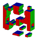
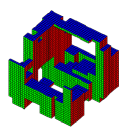
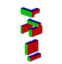
Figure 20: Example long-time states for a $32\times 32\times 8$ slab, a $32^{3}$ cube, and a $8\times 8\times 32$ bar.

It is striking that the three-dimensional system is so much more complicated than the corresponding two-dimensional case. This fact suggests that many more surprises await discovery for the kinetic Ising model in higher dimensions. Moreover, most of our findings are empirical in nature and they beg for the development of new theoretical perspective and geometrical descriptions of the domains. Another challenging extension of the present work is to describe the fate of spin systems with a non-scalar order parameter, such as the XY model, that are quenched to zero temperature

We gratefully acknowledge financial support from NSF grant DMR0906504 (JO and SR) and NSF grant CCF-0829541 (PLK).

Appendix A Accuracy of the Acceleration Algorithm

To test the accuracy of our acceleration algorithm, the system is evolved until a cutoff time $\tau$ with zero-temperature Glauber dynamics. Then at time $\tau$, an infinitesimal magnetic field is applied, that alternates as the system descends successive energy plateaux, until no flippable spins remain. Table 1 gives the final energy that is reached (where no flippable spins remain) when the acceleration algorithm is applied for different cutoff times $\tau$. These data are shown for the cases $L=10$, 20, and 100, with $10^{7}$, 10240, and 128 realizations, respectively. The extremely weak dependence of the final energy as a function of $\tau$ indicates the level of accuracy of the acceleration algorithm.

$L$	$\tau$	$\left<E_{L}\right>$	$R$
10	500	.4245900960
	$10^{9}$	.4245901020	34
	$10^{10}$	.4245901020	60
20	2000	.283285352
	$10^{5}$	.283287939	1.4
	$10^{6}$	.283287939	5.2
	$10^{7}$	.283287939	39
	$10^{8}$	.283288232	378
100	$5\times 10^{4}$	.083666469
	$10^{5}$	.083663406	1.2
	$5\times 10^{5}$	.083662656	4.7
	$10^{6}$	.083662594	7.2
	$10^{7}$	.083662531	67

Table 1: Average final energies $\langle E_{L}\rangle$ for different cutoff times $\tau$ and system sizes $L$.

The last column gives the ratio $R$ of the CPU time needed to simulate the system until no flippable spins remain when the acceleration algorithm is imposed at the cutoff time $\tau$ compared to imposing this algorithm at $\tau=5L^{2}$. For example, it took 67 times longer to simulate the $L=100$ system by running zero-temperature Glauber dynamics to $t=10^{7}$ and subsequently imposing the acceleration algorithm compared to running zero-temperature Glauber dynamics to $t=5\times 10^{4}$ and then imposing the acceleration algorithm. The relative difference in the energies by the two protocols is approximately $5\times 10^{-5}$, thus providing justification for our use of the acceleration algorithm at $t=5L^{2}$.

Appendix B Small Systems, Blinker States, Number of Clusters

The evolution of the smallest possible lattice $L=2$ helps to illustrate the complexities of larger systems. When $L=2$, there are 8 spins and $2^{8}=256$ possible states that can be enumerated to determine all details of the evolution. There are also only two possible final states: the ferromagnetic ground state (F) and a static metastable state (M) that consists of a square of four spins of one sign and an adjacent square of four spins of the opposite sign. There are nine distinct paths in state space that start at the antiferromagnetic state and end at these two final states (Table 2). The average survival time until the system reaches one of the final states is $\frac{221}{120}=1.841666\ldots$, while the probability of ultimately reaching the F final state is $\frac{11}{14}$.

path	# flips	time	prob.	final state
1	4	$\frac{43}{56}$	$\frac{2}{21}$	M
2	4	$\frac{143}{168}$	$\frac{1}{14}$	M
3	6	$\frac{341}{280}$	$\frac{1}{21}$	M
4	4	$\frac{85}{56}$	$\frac{3}{14}$	F
5	6	$\frac{1583}{840}$	$\frac{1}{35}$	F
6	6	$\frac{1793}{840}$	$\frac{4}{35}$	F
7	6	$\frac{127}{56}$	$\frac{4}{21}$	F
8	6	$\frac{395}{168}$	$\frac{1}{7}$	F
9	8	$\frac{761}{280}$	$\frac{2}{21}$	F

Table 2: The nine state-space paths to the final state for $L=2$ starting from the antiferromagnetic initial condition. Listed for each path are the number of spin flips until the final state is reached, the time to reach the final state on the path, and the probability of the path. Also listed is the final state for each path, either metastable (M) or ferromagnetic (F).

A complete enumeration is already not feasible for linear dimension $L=4$, where the number of states is $2^{64}\approx 1.84\times 10^{19}$; thus simulations are necessary when $L\geq 4$. For $L=4$, the average survival time is now 6.16, while the longest survival time observed in any realization is 22.2. For $L=6$ and 8, the respective average survival times are 11.9 and 27.9, while the longest survival times are 128 and $3.43\times 10^{6}$. For $L=10$, realizations that live beyond $t=10^{10}$ are possible, although rare, and it is not possible to quote an average survival time. The existence of such long-lived realizations for $L\geq 10$ contributes to the difficulty in the understanding of the behavior of the survival probability.

$L$	$P_{g}$	$P_{f}$	$P_{b}$
2	$\frac{11}{14}$	$\frac{3}{14}$	0
4	0.6814(1)	0.3186(1)	0
6	0.3523(2)	0.6353(2)	0.01246(4)
8	0.1842(1)	0.7373(1)	0.07853(9)
10	0.1045(1)	0.7170(1)	0.1785(1)
20	0.01377(4)	0.3059(1)	0.6803(1)
32	0.00322(8)	0.1091(4)	0.8877(4)
54	0.00066(6)	0.0406(4)	0.9587(4)
76	0.00040(6)	0.0250(5)	0.9746(5)
90	0.00039(6)	0.0199(4)	0.9797(4)

Table 3: Probabilities of reaching the ground state $P_{g}$, the frozen state $P_{f}$, and the blinker state $P_{b}$ versus $L$. The error in the last digit is shown in parentheses.

It is also worth noting that infinitely long-lived blinker states first appear for the case of $L=5$. Table 3 gives the data for the probabilities of reaching the ground state, a frozen static state, or a blinker state as a function of $L$. The former two probabilities decrease rapidly with $L$ and appear to approach zero for large $L$, while the probability that a blinker state is reached approaches 1 as $L$ increases (see also Fig. 6). As mentioned at the beginning of Sect. IV, the long-time state almost always consists of exactly two clusters. Table 4 gives the probabilities that the long-time state consists of one, two, three or more than three clusters as a function of $L$.

L	P(1)	P(2)	P(3)	P($>$3)
2	$\frac{11}{14}$	$\frac{3}{14}$	0	0
4	.6814(1)	.3186(1)	0	$<$.0000001
6	.3523(2)	.6475(2)	.000245(5)	$<$.0000001
8	.1842(1)	.8128(1)	.00303(2)	.0000004(2)
10	.1045(1)	.8866(1)	.00893(3)	.000015(1)
20	.01377(4)	.96052(6)	.02475(5)	.00096(1)
32	.00322(8)	.9720(2)	.0230(2)	.00180(6)
54	.00066(6)	.9802(3)	.0171(3)	.0020(1)
76	.00040(6)	.9824(4)	.0150(4)	.0022(1)
90	.00039(6)	.9839(4)	.0133(4)	.0024(2)

Table 4: Probabilities of reaching a state that contains 1, 2, 3, or $>3$ clusters at long times, with the error on the last digit in parentheses.

References

- (1) J. D. Gunton, M. San Miguel, and P. S. Sahni in: Phase Transitions and Critical Phenomena, Vol. 8, eds. C. Domb and J. L. Lebowitz (Academic, NY 1983);
- (2) A. J. Bray, Adv. Phys. 43, 357 (1994).
- (3) E. T. Gawlinski, M. Grant, J. D. Gunton, and K. Kaski, Phys. Rev. B 31, 281 (1985); J. Viñals and M. Grant, Phys. Rev. B 36, 7036 (1987).
- (4) P. L. Krapivsky, S. Redner and E. Ben-Naim, A Kinetic View of Statistical Physics (Cambridge: Cambridge University Press, 2010).
- (5) V. Spirin, P. L. Krapivsky, and S. Redner, Phys. Rev. E 63, 036118 (2001).
- (6) V. Spirin, P. L. Krapivsky, and S. Redner, Phys. Rev. E 6̱5, 016119 (2002).
- (7) P. Sundaramurthy and D. L. Stein, J. Phys. A 38, 349 (2005).
- (8) P. M. C. de Oliveira, C. M. Newman, V. Sidoravicious, and D. L. Stein, J. Phys. A: Math. Gen. 39, 6841 (2006).
- (9) K. Barros, P. L. Krapivsky, and S. Redner, Phys. Rev. E 80, 040101 (2009).
- (10) R. Morris, arXiv:0809.0353;
- (11) An abbreviated and preliminary account of this work is J. Olejarz, P. L. Krapivsky, and S. Redner, arXiv:1011.2903.
- (12) H. A. Schwarz, Gesammelte Mathematische Abhandlungen, Vol. 1, (Julius Springer, Berlin, 1890).
- (13) A. H. Schoen, Notices Amer. Math. Soc. 16, 19 (1969); A. H. Schoen, Infinite Periodic Minimal Surfaces without Self-Intersection, NASA Technical Note TN D-5541 (1970).
- (14) S. Leibler, in: Statistical Mechanics of Membranes and Surfaces, eds. by D. Nelson, T. Piran, and S. Weinberg (World Scientific, Teaneck, NJ, 1989), p. 45.
- (15) D. M. Anderson and P. Störm, in: Polymer Association Structures: Microemulsions and Liquid Crystals, ed. M. A. El-Nokaly, ACS Symposium Series No. 384 (American Chemical Society, Washington, DC, 1989), p. 204.
- (16) A. C. Finnefrock, R. Ulrich, G. E. S. Toombes, S. M. Gruner, and U. Wiesner, J. Am. Chem. Soc. 125, 13084 (2003).
- (17) M. Anderson, C. Egger, J. Casci, G. Tiddy, and K. Brakke, Angew. Chem. Int. Ed. 44, 2 (2005).
- (18) R. J. Glauber, J. Math. Phys. 4, 294 (1963).
- (19) N. Metropolis, A. W. Rosenbluth, M. N. Rosenbluth, A. H. Teller, and E. Teller, J. Chem. Phys. 21, 1087 (1953).
- (20) C. Godrèche and J. M. Luck, J. Phys.: Condens. Matter 17, S2573 (2005).
- (21) F. Ritort and P. Sollich, Adv. Phys. 52, 219 (2003).
- (22) J. Kurchan and L. Laloux, J. Phys. A 29, 1929 (1996).
- (23) D. S. Fisher, Physica D 107, 204 (1997).
- (24) J. Hoshen and R. Kopelman, Phys. Rev. B1 14 3438 (1976).
- (25) S. Redner, A Guide to First-Passage Processes (Cambridge University Press, New York, 2001).
- (26) J. D. Shore, M. Holzer, and J. P. Sethna, Phys. Rev. B 46, 11376 (1992).
- (27) A. Lipowski, Physica A 268, 6 (1999).
- (28) In contrast, final states are topologically trivial in two dimensions; the only possibilities are the ground state or a static metastable state that consists of an even number of straight stripes.
- (29) http://en.wikipedia.org/wiki/Eulercharacteristic.
- (30) K. Ueno, K. Shiga and S. Morita, A Mathematical Gift: The interplay between topology, functions, geometry, and algebra (AMS, Providence, R.I., 2003).
- (31) An exponential lower bound has been established by A. Pelletier (private communication), generalizing the weaker bound given in Ref. SKR01 . It is clear that for all .
- (32) C. M. Newman and D. L. Stein, Phys. Rev. Lett. 82, 3944 (1999); Physica A 279, 159 (2000).
- (33) http://en.wikipedia.org/wiki/Gauss-Bonnettheorem.
- (34) P. Svenson, Phys. Rev. E 64, 036122 (2001).
- (35) D. S. Dean, Eur. Phys. J. B 15, 493 (2000); A. Lefevre and D. S. Dean, Eur. Phys. J. B 21, 121 (2001).
- (36) C. Castellano and R. Pastor-Satorras, J. Stat. Mech. P05001 (2006).
- (37) C. P. Herrero, J. Phys. A 42, 415102 (2009).