A Robbins–Monro procedure for estimation in semiparametric regression models

Abstract

This paper is devoted to the parametric estimation of a shift together with the nonparametric estimation of a regression function in a semiparametric regression model. We implement a very efficient and easy to handle Robbins–Monro procedure. On the one hand, we propose a stochastic algorithm similar to that of Robbins–Monro in order to estimate the shift parameter. A preliminary evaluation of the regression function is not necessary to estimate the shift parameter. On the other hand, we make use of a recursive Nadaraya–Watson estimator for the estimation of the regression function. This kernel estimator takes into account the previous estimation of the shift parameter. We establish the almost sure convergence for both Robbins–Monro and Nadaraya–Watson estimators. The asymptotic normality of our estimates is also provided. Finally, we illustrate our semiparametric estimation procedure on simulated and real data.

and

1 Introduction

A wide range of real-life phenomena occur periodically. One can think about meteorology with daily or annual cycles of temperature MR2744122 , astronomy with the famous 11-year cycles of solar geomagnetic activity Lassen , medicine with human circadian rhythms Wang or ECG signals Trigano , econometry MR1623559 , MR833929 , communication MR2369028 , etc. Statistical analysis of periodic data is of great interest in order to design suitable models for those cyclic phenomena. An important literature is available on the so-called periodic shape-invariant model introduced by Lawton, Sylvestre and Maggio Lawton . Theoretical advances on shape-invariant models together with statistical applications may be found in MR1041386 , MR2744122 , MR1332581 , MR924858 , MR2662362 , Wang . A periodic shape-invariant model is a semiparametric regression model with an unknown periodic shape function. It is given, for all $n\geq 0$, by

$$Y_{n}=h(X_{n})+\varepsilon_{n},$$ (1)

where the inputs $(X_{n})$ are known observation times, the output $(Y_{n})$ are the observations, and $(\varepsilon_{n})$ are unknown random errors. The function $h$ is periodic and takes the form

$$h(x)=m+\sum_{k=1}^{p}a_{k}f(x-\theta_{k}),$$

where $f$ represents the unknown characteristic shape function, $m$ is the overall mean, while $\theta=(\theta_{1},\ldots,\theta_{p})$ and $a=(a_{1},\ldots,a_{p})$ are unknown shift and scale parameters.

In this paper, we shall focus our attention on the particular case $p=1$, $m=0$ and $a=1$ by studying the semiparametric regression model given, for all $n\geq 0$, by

$$Y_{n}=f(X_{n}-\theta)+\varepsilon_{n},$$ (2)

where $(X_{n})$ and $(\varepsilon_{n})$ are two independent sequences of independent and identically distributed random variables. We are dealing with random observation times in contrast with the previous literature where $(X_{n})$ are assumed to be known and equidistributed over a given interval. We are interested in the parametric estimation of the shift parameter $\theta$ together with the nonparametric estimation of the shape function $f$. However, one has to keep in mind that our main interest lies in the estimation of the parameter $\theta$. We are also motivated by a statistical application on the detection of atrial fibrillation using ECG analysis Clifford , Trigano .

First of all, we implement a Robbins–Monro procedure in order to estimate the unknown parameter $\theta$ without any preliminary evaluation of the regression function $f$. Our approach is very easy to handle and it performs very well. Moreover, our approach is totally different from the one recently proposed by Dalalyan, Golubev and Tsybakov MR2275239 in the Gaussian white-noise case. First, a penalized maximum likelihood estimator of $\theta$ is proposed in MR2275239 with an appropriately chosen penalty based on a Fourier series approximation of the function $f$. Second, the asymptotic behavior of the mean squared risk of this estimator is investigated. One can observe that our estimator is much easier to calculate. In addition, we do not require any assumption on the derivatives of the function $f$. In the situation where the parameter $\theta$ is random, Castillo and Loubes MR2508947 propose a plug-in version of the Parzen–Rosenblatt MR0143282 , MR0343355 density estimator of $\theta$. The construction of this estimate also relies on the penalized maximum likelihood estimator of $\theta$ given in MR2275239 . Furthermore, in the case where one observes several Gaussian functions differing from each other by a translation parameter, Gamboa, Loubes and Maza MR2369028 propose to transform the starting model by using a discrete Fourier transform. Hence, from the resulting model, they estimate the shift parameters by minimizing a quadratic functional. This approach is very interesting by the few assumptions made on the regression function. In a more general framework, Vimond MR2662362 makes use of a truncated Fourier approximation of $f$ in order to evaluate the profile log-likelihood score function associated with the shift and scale parameters. This two-step strategy requires, as in MR2369028 , the estimation of the Fourier coefficients of $f$. However, it performs pretty well as it leads to consistent and asymptotically efficient estimators of the shift and scale parameters. Our alternative approach to estimate $\theta$ is associated to a stochastic recursive algorithm similar to that of Robbins–Monro MR0042668 , MR0343355 .

Assume that one can find a function $\phi$, free of the parameter $\theta$, such that $\phi(\theta)=0$. Then, it is possible to estimate $\theta$ by the Robbins–Monro algorithm

$$\widehat{\theta}_{n+1}=\widehat{\theta}_{n}+\gamma_{n}T_{n+1},$$ (3)

where $(\gamma_{n})$ is a positive sequence of real numbers decreasing toward zero and $(T_{n})$ is a sequence of random variables such that $\mathbb{E}[T_{n+1}|\mathcal{F}_{n}]=\phi(\widehat{\theta}_{n})$ where $\mathcal{F}_{n}$ stands for the $\sigma$-algebra of the events occurring up to time $n$. Under standard conditions on the function $\phi$ and on the sequence $(\gamma_{n})$, it is well known MR1485774 , MR1993642 that $\widehat{\theta}_{n}$ tends to $\theta$ almost surely. The asymptotic normality of $\widehat{\theta}_{n}$ together with the quadratic strong law may also be found in MR624435 , MR2351104 and MR1654569 . A randomly truncated version of the Robbins–Monro algorithm is also given in MR931029 , MR2542461 .

Our second goal is the estimation of the unknown regression function $f$. A wide range of literature is available on nonparametric estimation of a regression function. We refer the reader to MR1843146 , MR2013911 for two excellent books on density and regression function estimation. Here, we focus our attention on the Nadaraya–Watson estimator of $f$. The almost sure convergence of the Nadaraya–Watson estimator MR0166874 , MR0185765 without the shift $\theta$ was established by Noda MR0426278 ; see also Härdle et al. MR740916 , MR964932 for the law of iterated logarithm and the uniform strong law. A nice extension of the previous results may be found in MR924860 . The asymptotic normality of the Nadaraya–Watson estimator was proved by Schuster MR0301845 . Moreover, Choi, Hall and Rousson MR1805786 propose three data-sharpening versions of the Nadaraya–Watson estimator in order to reduce the asymptotic variance in the central limit theorem. Furthermore, in the situation where the regression function is monotone, Hall and Huang MR1865334 provide a method for monotonizing the Nadaraya–Watson estimator. For $n$ large enough, their alternative estimator coincides with the standard Nadaraya–Watson estimator on a compact interval where the regression function $f$ is monotone. In our situation, we propose to make use of a recursive Nadaraya–Watson estimator MR1485774 of $f$ which takes into account the previous estimation of the shift parameter $\theta$. It is given, for all $x\in\mathbb{R}$, by

$$\widehat{f}_{n}(x)=\frac{\sum_{k=1}^{n}W_{k}(x)Y_{k}}{\sum_{k=1}^{n}W_{k}(x)}$$ (4)

with

$$W_{n}(x)=\frac{1}{h_{n}}K\biggl{(}\frac{X_{n}-\widehat{\theta}_{n-1}-x}{h_{n}}\biggr{)},$$

where the kernel $K$ is a chosen probability density function and the bandwidth $(h_{n})$ is a sequence of positive real numbers decreasing to zero. The main difficulty arising here is that we have to deal with the additional term $\widehat{\theta}_{n}$ inside the kernel $K$. Consequently, we are led to analyze a double stochastic algorithm with, at the same time, the study of the asymptotic behavior of the Robbins–Monro estimator $\widehat{\theta}_{n}$ of $\theta$, and the Nadaraya–Watson estimator $\widehat{f}_{n}$ of $f$.

The paper is organized as follows. Section 2 is devoted to the parametric estimation of $\theta$. We establish the almost sure convergence of $\widehat{\theta}_{n}$ as well as a law of iterated logarithm and the asymptotic normality. Section 3 deals with the nonparametric estimation of $f$. Under standard regularity assumptions on the kernel $K$, we prove the almost sure pointwise convergence of $\widehat{f}_{n}$ to $f$. In addition, we also establish the asymptotic normality of $\widehat{f}_{n}$. Section 4 contains some numerical experiments on simulated and real ECG data, illustrating the performances of our semiparametric estimation procedure. The proofs of the parametric results are given in Section 5, while those concerning the nonparametric results are postponed to Section 6.

2 Estimation of the shift

First of all, we focus our attention on the estimation of the shift parameter $\theta$ in the semiparametric regression model given by (2). We assume that $(\varepsilon_{n})$ is a sequence of independent and identically distributed random variables with zero mean and unknown positive variance $\sigma^{2}$. Moreover, it is necessary to make several hypotheses similar to those of MR2275239 .

($$\mathcal{H}_{9}$$)

Let $X$ be a random variable sharing the same distribution as $(X_{n})$. In all the sequel, the auxiliary function $\phi$ defined, for all $t\in\mathbb{R}$, by

$$\phi(t)=\mathbb{E}\biggl{[}\frac{\sin(2\pi(X-t))}{g(X)}f(X-\theta)\biggr{]}$$ (1)

will play a prominent role. More precisely, it follows from the periodicity of $f$ that

$$\phi(t) = \int_{-1/2}^{1/2}\sin\bigl{(}2\pi(x-t)\bigr{)}f(x-\theta)\,dx$$

$$= \int_{-1/2}^{1/2}\sin\bigl{(}2\pi(y+\theta-t)\bigr{)}f(y)\,dy,$$

$$= \sin\bigl{(}2\pi(\theta-t)\bigr{)}\int_{-1/2}^{1/2}\cos(2\pi y)f(y)\,dy$$

$${}+\cos\bigl{(}2\pi(\theta-t)\bigr{)}\int_{-1/2}^{1/2}\sin(2\pi y)f(y)\,dy.$$

Consequently, the symmetry of $f$ leads to

$$\phi(t)=f_{1}\sin\bigl{(}2\pi(\theta-t)\bigr{)},$$ (2)

where $f_{1}$ is the first Fourier coefficient of $f$

$$f_{1}=\int_{-1/2}^{1/2}\cos(2\pi x)f(x)\,dx.$$

Throughout the paper, we assume that $f_{1}\neq 0$. Obviously, $\phi$ is a continuous and bounded function such that $\phi(\theta)=0$. In addition, one can easily verify that for all $t\in\mathbb{R}$ such that $|t-\theta|<1/2$, the product $(t-\theta)\phi(t)$ has a constant sign. It is negative if $f_{1}>0$, while it is positive if $f_{1}<0$. Therefore, we are in position to implement our Robbins–Monro procedure MR0042668 , MR0343355 . Let $K=[-1/4,1/4]$ and denote by $\pi_{K}$ the projection on the compact set $K$ defined, for all $x\in\mathbb{R}$, by

$$\pi_{K}(x)=\cases{x,&\quad if $|x|\leq 1/4$,\cr 1/4,&\quad if $x\geq 1/4$,\cr-1/4,&\quad if $x\leq-1/4$.}$$

Let $(\gamma_{n})$ be a decreasing sequence of positive real numbers satisfying

$$\sum_{n=1}^{\infty}\gamma_{n}=+\infty\quad\mbox{and}\quad\sum_{n=1}^{\infty}\gamma_{n}^{2}<+\infty.$$ (3)

For the sake of clarity, we shall make use of $\gamma_{n}=1/n$. We estimate the shift parameter $\theta$ via the projected Robbins–Monro algorithm

$$\widehat{\theta}_{n+1}=\pi_{K}\bigl{(}\widehat{\theta}_{n}+\operatorname{sign}(f_{1})\gamma_{n+1}T_{n+1}\bigr{)},$$ (4)

where the initial value $\widehat{\theta}_{0}\in K$ and the random variable $T_{n+1}$ is defined by

$$T_{n+1}=\frac{\sin(2\pi(X_{n+1}-\widehat{\theta}_{n}))}{g(X_{n+1})}Y_{n+1}.$$ (5)

Our first result concerns the almost sure convergence of the estimator $\widehat{\theta}_{n}$.

Theorem 2.1

Assume that ($\mathcal{H}_{9}$) and ($\mathcal{H}_{9}$) hold and that $|\theta|<1/4$. Then, $\widehat{\theta}_{n}$ converges almost surely to $\theta$. In addition, the number of times that the random variable $\widehat{\theta}_{n}+\operatorname{sign}(f_{1})\gamma_{n+1}T_{n+1}$ goes outside of $K$ is almost surely finite.

In order to establish the asymptotic normality of $\widehat{\theta}_{n}$, it is necessary to introduce a second auxiliary function $\varphi$ defined, for all $t\in\mathbb{R}$, by

$$\varphi(t) = \mathbb{E}\biggl{[}\frac{\sin^{2}(2\pi(X-t))}{g^{2}(X)}\bigl{(}f^{2}(X-\theta)+\sigma^{2}\bigr{)}\biggr{]}$$

$$= \int_{-1/2}^{1/2}\frac{\sin^{2}(2\pi(x-t))}{g(x)}\bigl{(}f^{2}(x-\theta)+\sigma^{2}\bigr{)}\,dx.$$

As soon as $4\pi|f_{1}|>1$, denote

$$\xi^{2}(\theta)=\frac{\varphi(\theta)}{4\pi|f_{1}|-1}.$$ (7)

Theorem 2.2

Assume that ($\mathcal{H}_{9}$) and ($\mathcal{H}_{9}$) hold and that $|\theta|<1/4$. In addition, suppose that $(\varepsilon_{n})$ has a finite moment of order $>2$ and that $4\pi|f_{1}|>1$. Then, we have the asymptotic normality

$$\sqrt{n}(\widehat{\theta}_{n}-\theta)\stackrel{{\scriptstyle\mathcal{L}}}{{\longrightarrow}}\mathcal{N}(0,\xi^{2}(\theta)).$$ (8)

Remark 2.1.

We clearly have $\phi^{\prime}(t)=-2\pi f_{1}\cos(2\pi(\theta-t)).$ Consequently, the value $\phi^{\prime}(\theta)=-2\pi f_{1}$ does not depend upon the unknown parameter $\theta$. On the one hand, if the first Fourier coefficient $f_{1}$ of $f$ is known, it is possible to provide, via a slight modification of (4), an asymptotically efficient estimator $\widehat{\theta}_{n}$ of $\theta$. More precisely, it is only necessary to replace $\gamma_{n}=1/n$ in (4) by $\gamma_{n}=\gamma/n$ where

$$\gamma=\frac{1}{2\pi|f_{1}|}.$$

Then, we deduce from the original work of Fabian MR0381189 that $\widehat{\theta}_{n}$ is an asymptotically efficient estimator of $\theta$ with

$$\sqrt{n}(\widehat{\theta}_{n}-\theta)\stackrel{{\scriptstyle\mathcal{L}}}{{\longrightarrow}}\mathcal{N}\biggl{(}0,\frac{\varphi(\theta)}{4\pi^{2}f_{1}^{2}}\biggr{)}.$$ (9)

On the other hand, if $f_{1}$ is unknown, it is also possible to provide by the same procedure an asymptotically efficient estimator $\widehat{\theta}_{n}$ of $\theta$ replacing $f_{1}$ by its natural estimate

$$\widehat{f}_{1,n}=\frac{1}{n}\sum_{k=1}^{n}\frac{Y_{k}\cos(2\pi(X_{k}-\widehat{\theta}_{k-1}))}{g(X_{k})}.$$

Remark 2.2.

In the particular case where $4\pi|f_{1}|=1$, it is also possible to show MR1485774 that

$$\sqrt{\frac{n}{\log(n)}}(\widehat{\theta}_{n}-\theta)\stackrel{{\scriptstyle\mathcal{L}}}{{\longrightarrow}}\mathcal{N}(0,\varphi(\theta)).$$

Asymptotic results are also available when $0<4\pi|f_{1}|<1$. However, we have chosen to focus our attention on the more attractive case $4\pi|f_{1}|>1$.

Theorem 2.3

Assume that ($\mathcal{H}_{9}$) and ($\mathcal{H}_{9}$) hold and that $|\theta|<1/4$. In addition, suppose that $(\varepsilon_{n})$ has a finite moment of order $>2$ and that $4\pi|f_{1}|>1$. Then, we have the law of iterated logarithm

$$\limsup_{n\rightarrow\infty}\biggl{(}\frac{n}{2\log\log n}\biggr{)}^{1/2}(\widehat{\theta}_{n}-\theta) = -\liminf_{n\rightarrow\infty}\biggl{(}\frac{n}{2\log\log n}\biggr{)}^{1/2}(\widehat{\theta}_{n}-\theta)$$

$$= \xi(\theta)\qquad\mbox{a.s.}$$

In particular,

$$\limsup_{n\rightarrow\infty}\biggl{(}\frac{n}{2\log\log n}\biggr{)}(\widehat{\theta}_{n}-\theta)^{2}=\xi^{2}(\theta)\qquad\mbox{a.s.}$$ (11)

In addition, we also have the quadratic strong law

$$\lim_{n\rightarrow\infty}\frac{1}{\log n}\sum_{k=1}^{n}(\widehat{\theta}_{k}-\theta)^{2}=\xi^{2}(\theta)\qquad\mbox{a.s.}$$ (12)

The proofs are given in Section 5.

Remark 2.3.

It is also possible to get rid of the symmetry assumption on $f$. However, it requires the knowledge of the first Fourier coefficients of $f$:

$$f_{1}=\int_{-1/2}^{1/2}\cos(2\pi x)f(x)\,dx\quad\mbox{and}\quad g_{1}=\int_{-1/2}^{1/2}\sin(2\pi x)f(x)\,dx.$$

On the one hand, it is necessary to assume that $f_{1}\neq 0$ or $g_{1}\neq 0$, and to replace the first auxiliary function $\phi$ defined in (1) by

$$\Phi(t) = f_{1}\mathbb{E}\biggl{[}\frac{\sin(2\pi(X-t))}{g(X)}f(X-\theta)\biggr{]}-g_{1}\mathbb{E}\biggl{[}\frac{\cos(2\pi(X-t))}{g(X)}f(X-\theta)\biggr{]}$$

$$= (f_{1}^{2}+g_{1}^{2})\sin\bigl{(}2\pi(\theta-t)\bigr{)}.$$

Then, Theorem 2.1 is true for the projected Robbins–Monro algorithm

$$\widehat{\theta}_{n+1}=\pi_{K}(\widehat{\theta}_{n}+\gamma_{n+1}T_{n+1}),$$

where the initial value $\widehat{\theta}_{0}\in K$ and the random variable $T_{n+1}$ is defined by

$$T_{n+1}=\frac{f_{1}\sin(2\pi(X_{n+1}-\widehat{\theta}_{n}))}{g(X_{n+1})}Y_{n+1}-\frac{g_{1}\cos(2\pi(X_{n+1}-\widehat{\theta}_{n}))}{g(X_{n+1})}Y_{n+1}.$$

On the other hand, we also have to replace the second function $\varphi$ defined in (2) by

$$\Psi(t) = \mathbb{E}\biggl{[}\frac{(f_{1}\sin(2\pi(X-t))-g_{1}\cos(2\pi(X-t)))^{2}}{g^{2}(X)}\bigl{(}f^{2}(X-\theta)+\sigma^{2}\bigr{)}\biggr{]}$$

$$= \int_{-1/2}^{1/2}\frac{(f_{1}\sin(2\pi(x-t))-g_{1}\cos(2\pi(x-t)))^{2}}{g(x)}\bigl{(}f^{2}(x-\theta)+\sigma^{2}\bigr{)}\,dx.$$

Then, as soon as $4\pi(f_{1}^{2}+g_{1}^{2})>1$, Theorems 2.2 and 2.3 hold with

$$\xi^{2}(\theta)=\frac{\Psi(\theta)}{4\pi(f_{1}^{2}+g_{1}^{2})-1}.$$

In the rest of the paper, we shall not go in that direction as our strategy is to make very few assumptions on the Fourier coefficients of $f$.

3 Estimation of the regression function

This section is devoted to the nonparametric estimation of the regression function $f$ via a recursive Nadaraya–Watson estimator. On the one hand, we add the standard hypothesis:

$$\mbox{The regression function~{}$f$ is Lipschitz}.\hskip 110.0pt \mathcal{H}_{3}$$ ()

On the other hand, we recall that under ($\mathcal{H}_{9}$), the function $f$ is assumed to be symmetric. Consequently, we follow the same approach as the one developed by Stone MR0362669 for the estimation of a symmetric probability density function replacing the estimator (4) by its symmetrized version

$$\widehat{f}_{n}(x)=\frac{\sum_{k=1}^{n}(W_{k}(x)+W_{k}(-x))Y_{k}}{\sum_{k=1}^{n}(W_{k}(x)+W_{k}(-x))},$$ (1)

where

$$W_{n}(x)=\frac{1}{h_{n}}K\biggl{(}\frac{X_{n}-\widehat{\theta}_{n-1}-x}{h_{n}}\biggr{)}.$$

The bandwidth $(h_{n})$ is a sequence of positive real numbers, decreasing to zero, such that $nh_{n}$ tends to infinity. For the sake of simplicity, we propose to make use of $h_{n}=1/n^{\alpha}$ with $\alpha\in\ ]0,1[$. Moreover, we shall assume in all the sequel that the kernel $K$ is a positive symmetric function, bounded with compact support, twice differentiable with bounded derivatives, satisfying

$$\int_{\mathbb{R}}K(x)\,dx=1\quad\mbox{and}\quad\int_{\mathbb{R}}K^{2}(x)\,dx=\nu^{2}.$$

Our next result deals with the almost sure convergence of the estimator $\widehat{f}_{n}$.

Theorem 3.1

Assume that ($\mathcal{H}_{9}$), ($\mathcal{H}_{9}$) and ($\mathcal{H}_{3}$) hold and that $|\theta|<1/4$ and the sequence $(\varepsilon_{n})$ has a finite moment of order $>2$. Then, for any $x\in\mathbb{R}$ such that $|x|\leq{1/2}$,

$$\lim_{n\rightarrow\infty}\widehat{f}_{n}(x)=f(x)\qquad\mbox{a.s.}$$ (2)

The asymptotic normality of the estimator $\widehat{f}_{n}$ is as follows.

Theorem 3.2

Assume that ($\mathcal{H}_{9}$), ($\mathcal{H}_{9}$) and ($\mathcal{H}_{3}$) hold and that $|\theta|<1/4$ and the sequence $(\varepsilon_{n})$ has a finite moment of order $>2$. Then, as soon as the bandwidth $(h_{n})$ satisfies $h_{n}=1/n^{\alpha}$ with $\alpha>1/3$, we have for any $x\in\mathbb{R}$ such that $|x|\leq{1/2}$ with $x\neq{0}$, the pointwise asymptotic normality

$$\sqrt{nh_{n}}\bigl{(}\widehat{f}_{n}(x)-f(x)\bigr{)}\stackrel{{\scriptstyle\mathcal{L}}}{{\longrightarrow}}\mathcal{N}\biggl{(}0,\frac{\sigma^{2}\nu^{2}}{(1+\alpha)(g(\theta+x)+g(\theta-x))}\biggr{)}.$$ (3)

In addition, for $x=0$,

$$\sqrt{nh_{n}}\bigl{(}\widehat{f}_{n}(0)-f(0)\bigr{)}\stackrel{{\scriptstyle\mathcal{L}}}{{\longrightarrow}}\mathcal{N}\biggl{(}0,\frac{\sigma^{2}\nu^{2}}{(1+\alpha)g(\theta)}\biggr{)}.$$ (4)

The proofs are given in Section 6.

4 Simulations

The goal of this section is to illustrate via some numerical experiments the good performances of our estimation strategy. The first subsection is devoted to simulated data created according to the model (2) while the second one deals with real ECG data taken from the MIT-BIH database. Our aim is to propose an efficient and easy to handle procedure in order to detect atrial fibrillation using ECG records. An interesting study on ECG analysis in order to detect cardiac arrhythmia may also be found in Trigano .

4.1 Simulated data

Consider the semiparametric regression model

$$Y_{n}=f(X_{n}-\theta)+\varepsilon_{n},$$

where $\theta=1/10$ and the periodic shape function $f$ is given, for $p\geq 1$ and for all $x\in\mathbb{R}$, by

$$f(x)=\sum_{k=1}^{p}\cos(2k\pi x)$$

with $p=8$. We have chosen $(X_{n})$ and $(\varepsilon_{n})$ as two independent sequences of independent random variables with $\mathcal{U}[-1/2,1/2]$ and $\mathcal{N}(0,1)$ distributions, respectively. The simulated data are given in the left-hand side of Figure 1.

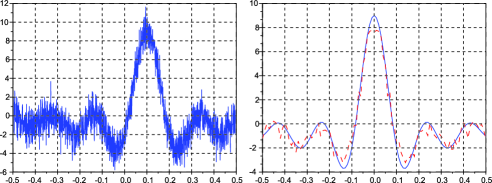
Figure 1: Simulated data and almost sure convergence.

For the estimation of the shift parameter $\theta$, we implement our Robbins–Monro procedure with $n=1000$ iterations. We obtain the estimate $\widehat{\theta}_{n}=0.1014$ which shows the good asymptotic behavior of the estimator $\widehat{\theta}_{n}$ comparing to the true value $\theta=1/10$. Moreover, using convergence (8), one can obtain confidence intervals for the shift parameter. More precisely, they are given, for all $n\geq 1$, by

$$I_{n}(\theta)=\biggl{[}\widehat{\theta}_{n}-q_{\beta}\frac{\widehat{\xi}_{n}(\theta)}{\sqrt{n}},\widehat{\theta}_{n}+q_{\beta}\frac{\widehat{\xi}_{n}(\theta)}{\sqrt{n}}\biggr{]},$$

where $q_{\beta}$ stands for the quantile of order $0<\beta<1$ of the $\mathcal{N}(0,1)$ distribution and $\widehat{\xi}_{n}(\theta)$ is a consistent estimator of $\xi(\theta)$ given by (7). In our particular case, it is not necessary to estimate $\xi^{2}(\theta)$ since via straightforward calculations, $f_{1}=1/2$ and

$$\xi^{2}(\theta)=\frac{7}{8(2\pi-1)}.$$

Moreover, for $n=1000$ and for a risk $\beta=5\%$, the confidence interval is precisely $I_{n}(\theta)=[0.0762;0.1266]$. The length of $I_{n}(\theta)$ is 0.0504, which is rather small, so our Robbins–Monro procedure performs pretty well. All confidence intervals $I_{n}(\theta)$, for $n=1,\ldots,1000$, are drawn in red in the left-hand side of Figure 2.

For the estimation of the regression function $f$, we make use of the uniform kernel $K$ on the interval $[-1,1]$, and the bandwidth $h_{n}=1/n^{\alpha}$ with $\alpha=9/10$. In addition, it follows from convergences (3) and (4) that for $n=1000$ and for all $x\in{[-1/2,1/2]}$, a confidence interval for $f(x)$ is given by

$$J_{n}(x)=\biggl{[}\widehat{f}_{n}(x)-q_{\beta}\frac{\widehat{v}_{n}(x,\widehat{\theta}_{n})}{\sqrt{nh_{n}}},\widehat{f}_{n}(x)+q_{\beta}\frac{\widehat{v}_{n}(x,\widehat{\theta}_{n})}{\sqrt{nh_{n}}}\biggr{]},$$

where $q_{\beta}$ stands for the quantile of order $0<\beta<1$ of the $\mathcal{N}(0,1)$ distribution and $\widehat{v}_{n}^{2}(x,\widehat{\theta}_{n})$ is a consistent estimator of the asymptotic variance $v^{2}(x,\theta)$ in Theorem 3.2. In our particular case, $\nu^{2}=1/2$ and

$$v^{2}(x,\theta)=\cases{5/19,&\quad if $-1/2\leq{x}<-2/$ or $2/5<x\leq 1/2$,\cr 5/38,&\quad if $-2/5\leq{x}\leq 2/5$ and $x\neq 0$,\cr 5/19,&\quad if $x=0$.}$$

All confidence intervals $J_{n}(x)$, for all $x\in{}[-1/2,1/2]$, are drawn in red in the right-hand side of Figure 2. On the one hand, the simulations show that the largest length of the confidence intervals $J_{n}(x)$ is for $x=-0.47$ and $x=0.47$ and the length is precisely equal to $1.0066$. On the other hand, the smallest length of the confidence intervals $J_{n}(x)$ is for $x=-0.04$ and $x=0.04$ and is equal to $0.7118$. The fact that there are two values of $x$ for the largest and the smallest length of confidence intervals is due to the symmetry of the estimator $\widehat{f}_{n}$. Then, one can observe on this first set of simulated data that the Robbins–Monro estimator $\widehat{\theta}_{n}$ of $\theta$ as well as the Nadaraya–Watson estimator $\widehat{f}_{n}$ of $f$ perform pretty well.

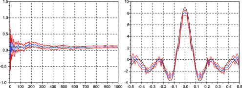
Figure 2: Confidence intervals for $\theta$ and $f$.

Our second experiment deals with $30$ curves according to the model

$$Y_{n}=f(X_{n}-\theta)+\varepsilon_{n},$$

where $\theta=-1/5$ for the first $10$ curves and $\theta^{\prime}=1/10$ for the last $20$ curves. The periodic shape function $f$ is given, for all $x\in[-1/2,1/2]$, by

$$f(x)=\cos(2\pi x)+\sin(2\pi x)+\cos(2\pi x)\sin(2\pi x).$$

Our goal is to propose a statistical procedure in order to detect a lag between the first $10$ curves with $\theta=-1/5$ and the last $20$ curves with $\theta^{\prime}=1/10$. In other words, we want to observe whether or not the value $\Delta=\theta^{\prime}-\theta$ is far away from zero. We have chosen $(X_{n})$ and $(\varepsilon_{n})$ as two independent sequences of independent and Gaussian random variables with uniform distribution on $[-1/2,1/2]$ and $\mathcal{N}(0,1/5)$ distribution, respectively. Each curve is drawn with $n=200$ points. The different curves are given in Figure 3.

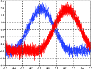
Figure 3: Simulated data with two different values $\theta$ and $\theta^{\prime}$.

On the one hand, we estimate the first value $\theta=-1/5$ from the first $10$ curves. We implement our Robbins–Monro procedure with $n=200$ iterations for the first estimate $\widehat{\theta}_{n}$ of $\theta$ evaluated on the first curve, then with $n=400$ iterations for the second estimate $\widehat{\theta}_{n}$ of $\theta$ evaluated on the two first curves, and so on, until the calculation of the last estimate $\widehat{\theta}_{n}$ of $\theta$ with $n=2000$. Therefore, we obtain $-0.1950$ for the arithmetic mean of the first $10$ estimates $\widehat{\theta}_{n}$ of $\theta$. We continue with the same procedure on all the set of curves. The value of the eleven estimates with $n=2200$ is $0.0986$. This value is significantly different from the first $10$ estimates. It corresponds to the first curve simulated with $\theta^{\prime}=1/10$. Furthermore, we obtain $0.0998$ for the arithmetic mean of the last $20$ estimates $\widehat{\theta}_{n}$ of $\theta^{\prime}$. Finally, our statistical procedure allows us to detect a change of parameterization from the value $\theta=-1/5$ to the value $\theta^{\prime}=1/10$ as $\widehat{\Delta}_{n}=0.0998+0.1950=0.2948$. In order to compute more accurate values of $\widehat{\theta}_{n}$, one can replace $\gamma_{n}=1/n$ in (4) by $\gamma_{n}=1/n^{a}$ where $1/2<a<1$. This will be done for the implementation of our Robbins–Monro procedure on real ECG data.

4.2 Real ECG data

We shall now focus our attention on real ECG data. We have chosen the record $04015$ in the Atrial Fibrillation (AF) database provided by MIT-BIH database. Each recording consists in a continuous digitized ECG signal measured over 1 hour in order to detect AF which is the most common cardiac arrythmia. A stronger indicator of AF is the absence of P waves or the irregularities of RR interval on an electrocardiogram. We refer the reader to Clifford for an interesting book on statistical methods and tools for ECG data analysis. Our aim is to propose a statistical procedure in order to detect irregularities of RR interval on the ECG record $04015$. The record and its projection on the interval $[-1/2,1/2]$ are given in Figure 4. The size of the data set is $2038$. We assume that the model

$$Y_{n}=f(X_{n}-\theta)+\varepsilon_{n}$$

fits the data, where the sequence $(X_{n})$ is uniformly distributed over the interval $[-1/2,1/2]$. The periodic shape function $f$ is clearly not symmetric. However, we already saw in Remark 2.3 that our Robbins–Monro procedure still holds for nonsymmetric regression function.

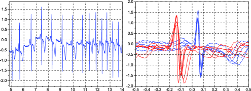
Figure 4: Original data.

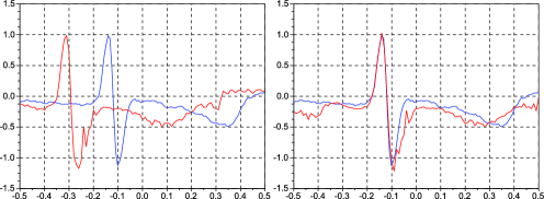
Figure 5: Reconstruction of the ECG.

As for simulated data, in view of the signal, we would find two different values $\theta$ and $\theta^{\prime}$. The first value $\theta$ is associated with the first part of the signal, while the second value $\theta^{\prime}$ corresponds to the second part. The difference $\Delta=\theta^{\prime}-\theta$ between the two parameters would explain the lag between the two parts of the signal. A value of $\Delta$ far away from zero could be interpreted as the detection of irregularities of RR interval which confirms the diagnostic of atrial fibrillation. On this record, our Robbins–Monro procedure with $n=800$ iterations leads to the first estimate $\widehat{\theta}_{n}=0.1734$ for $\theta$ and the last estimate $\widehat{\theta}_{n}=-0.0092$ for $\theta^{\prime}$ with $n=1238$. The value $\widehat{\Delta}_{n}=-0.0092-0.1734=-0.1826$ explains the lag in Figure 4. Figure 5 shows that our Nadaraya–Watson procedure for the reconstruction of ECG signals works pretty well.

5 Proofs of the parametric results

5.1 Proof of Theorem 2.1

We can assume without loss of generality that $f_{1}>0$ inasmuch as the proof for $f_{1}<0$ follows exactly the same lines. Denote by $\mathcal{F}_{n}$ the $\sigma$-algebra of the events occurring up to time $n$, $\mathcal{F}_{n}=\sigma(X_{0},\varepsilon_{0},\ldots,X_{n},\varepsilon_{n})$. First of all, we shall calculate the two first conditional moments of the random variable $T_{n}$ given by (5). It follows from (2) that

$$\mathbb{E}[T_{n+1}|\mathcal{F}_{n}] = \mathbb{E}\biggl{[}\frac{\sin(2\pi(X_{n+1}-\widehat{\theta}_{n}))Y_{n+1}}{g(X_{n+1})}\Big{|}\mathcal{F}_{n}\biggr{]}$$

$$= \mathbb{E}\biggl{[}\frac{\sin(2\pi(X_{n+1}-\widehat{\theta}_{n}))(f(X_{n+1}-\theta)+\varepsilon_{n+1})}{g(X_{n+1})}\Big{|}\mathcal{F}_{n}\biggr{]}.$$

On the one hand, as $(X_{n})$ is a sequence of independent random variables sharing the same distribution as a random variable $X$, we have

$$\qquad\mathbb{E}\biggl{[}\frac{\sin(2\pi(X_{n+1}-\widehat{\theta}_{n}))f(X_{n+1}-\theta)}{g(X_{n+1})}\Big{|}\mathcal{F}_{n}\biggr{]}=\phi(\widehat{\theta}_{n})\qquad\mbox{a.s.},$$ (5)

where $\phi$ is the function given by (1). On the other hand, as $(X_{n})$ and $(\varepsilon_{n})$ are two independent sequences and $(\varepsilon_{n})$ is a sequence of independent and square integrable random variables with zero mean, we also have

$$\mathbb{E}\biggl{[}\frac{\sin(2\pi(X_{n+1}-\widehat{\theta}_{n}))\varepsilon_{n+1}}{g(X_{n+1})}\Big{|}\mathcal{F}_{n}\biggr{]}=\mathbb{E}\biggl{[}\frac{\sin(2\pi(X-\widehat{\theta}_{n}))}{g(X)}\biggr{]}\mathbb{E}[\varepsilon_{n+1}]=0.$$

Hence, (5) leads to

$$\mathbb{E}[T_{n+1}|\mathcal{F}_{n}]=\phi(\widehat{\theta}_{n})\qquad\mbox{a.s.}$$ (6)

On the other hand,

$$T_{n+1}^{2} = \frac{\sin^{2}(2\pi(X_{n+1}-\widehat{\theta}_{n}))Y_{n+1}^{2}}{g^{2}(X_{n+1})}$$

$$= \frac{\sin^{2}(2\pi(X_{n+1}-\widehat{\theta}_{n}))(f^{2}(X_{n+1}-\theta)+2\varepsilon_{n+1}f(X_{n+1}-\theta)+\varepsilon_{n+1}^{2})}{g^{2}(X_{n+1})}.$$

Consequently, as the function $f$ is bounded, the density $g$ is positive on $[-1/2,1/2]$, and $\mathbb{E}[\varepsilon_{n+1}^{2}|\mathcal{F}_{n}]=\mathbb{E}[\varepsilon_{n+1}^{2}]=\sigma^{2}$, we obtain that

$$\qquad\mathbb{E}[T_{n+1}^{2}|\mathcal{F}_{n}]=\mathbb{E}\biggl{[}\frac{\sin^{2}(2\pi(X-\widehat{\theta}_{n}))}{g^{2}(X)}\bigl{(}f^{2}(X-\theta)+\sigma^{2}\bigr{)}\biggr{]}=\varphi(\widehat{\theta}_{n}),$$ (7)

where $\varphi$ is given by (2). Therefore, as $f$ is bounded and $g$ does not vanish on its support $[-1/2,1/2]$, we deduce from (7) that for some constant $M>0$

$$\sup_{n\geq 0}\mathbb{E}[T_{n+1}^{2}|\mathcal{F}_{n}]\leq M\qquad\mbox{a.s.}$$ (8)

Furthermore, for all $n\geq 0$, let $V_{n}=(\widehat{\theta}_{n}-\theta)^{2}$. We clearly have

$$V_{n+1} = (\widehat{\theta}_{n+1}-\theta)^{2}$$

$$= \bigl{(}\pi_{K}(\widehat{\theta}_{n}+\gamma_{n+1}T_{n+1})-\theta\bigr{)}^{2}$$

$$= \bigl{(}\pi_{K}(\widehat{\theta}_{n}+\gamma_{n+1}T_{n+1})-\pi_{K}(\theta)\bigr{)}^{2}$$

as we have assumed that $\theta$ belongs to $K$. Since $\pi_{K}$ is a Lipschitz function with Lipschitz constant $1$, we obtain that

$$V_{n+1} \leq (\widehat{\theta}_{n}+\gamma_{n+1}T_{n+1}-\theta)^{2}$$

$$\leq V_{n}+\gamma_{n+1}^{2}T_{n+1}^{2}+2\gamma_{n+1}T_{n+1}(\widehat{\theta}_{n}-\theta).$$

Hence, it follows from (6) and (8) that

$$\mathbb{E}[V_{n+1}|\mathcal{F}_{n}] \leq V_{n}+\gamma_{n+1}^{2}\mathbb{E}[T_{n+1}^{2}|\mathcal{F}_{n}]+2\gamma_{n+1}(\widehat{\theta}_{n}-\theta)\mathbb{E}[T_{n+1}|\mathcal{F}_{n}]$$

$$\leq V_{n}+\gamma_{n+1}^{2}M+2\gamma_{n+1}(\widehat{\theta}_{n}-\theta)\phi(\widehat{\theta}_{n})\qquad\mbox{a.s.}$$

In addition, as $\widehat{\theta}_{n}\in K$, $|\widehat{\theta}_{n}|<1/4$, $|\widehat{\theta}_{n}-\theta|<1/2$ which implies that $(\widehat{\theta}_{n}-\theta)\phi(\widehat{\theta}_{n})<0$. Then, we deduce from (5.1) together with the Robbins–Siegmund theorem (see Duflo MR1485774 , page 18) that the sequence $(V_{n})$ converges a.s. to a finite random variable $V$ and

$$\sum_{n=1}^{\infty}\gamma_{n+1}(\theta-\widehat{\theta}_{n})\phi(\widehat{\theta}_{n})<+\infty\qquad\mbox{a.s.}$$ (10)

Assume by contradiction that $V\neq 0$ a.s. Then, one can find $0<a<b<1/2$ such that, for $n$ large enough, the event $\{a<|\widehat{\theta}_{n}-\theta|<b\}$ is not negligible. However, on this annulus, one can also find some constant $c>0$ such that $(\theta-\widehat{\theta}_{n})\phi(\widehat{\theta}_{n})>c$ which, by (10), implies that

$$\sum_{n=1}^{\infty}\gamma_{n}<+\infty.$$

This is of course in contradiction with assumption (3). Consequently, it follows that $V=0$ a.s. leading to the almost sure convergence of $\widehat{\theta}_{n}$ to $\theta$.
It remains to show that $\widehat{\theta}_{n}+\gamma_{n+1}T_{n+1}$ goes almost surely outside of $K$ a finite number of times. For all $n\geq 1$, denote

$$N_{n}=\sum_{k=0}^{n-1}\mathrm{I}_{\{|\widehat{\theta}_{k}+\gamma_{k+1}T_{k+1}|>1/4\}}.$$

The random sequence $(N_{n})$ is nondecreasing. Assume by contradictionthat $N_{n}$ goes to infinity a.s. Then, one can find a subsequence $(n_{k})$ such that $(N_{n_{k}})$ is increasing. Consequently, for all $n_{k}>0$,

$$|\widehat{\theta}_{n_{k}}+\gamma_{n_{k}+1}T_{n_{k}+1}|>\tfrac{1}{4}\qquad\mbox{a.s.},$$

which implies that $|\widehat{\theta}_{n_{k}+1}|=1/4$ a.s. Hence,

$$\lim_{n_{k}\rightarrow\infty}|\widehat{\theta}_{n_{k}}|=|\theta|=\frac{1}{4}\qquad\mbox{a.s.}$$

leading to a contradiction as $|\theta|<1/4$. Finally, $(N_{n})$ converges to a finite limiting value a.s. which completes the proof of Theorem 2.1.

5.2 Proof of Theorem 2.2

We assume without loss of generality that $f_{1}>0$. Our goal is to apply Theorem 2.1 of Kushner and Yin (MR1993642 , page 330). First of all, as $\gamma_{n}=1/n$, the condition on the decreasing step is satisfied. Moreover, we already saw that $\widehat{\theta}_{n}$ converges almost surely to $\theta$. Consequently, all the local assumptions of Theorem 2.1 of MR1993642 are satisfied. In addition, it follows from $(\ref{meanTn})$ that $\mathbb{E}[T_{n+1}|\mathcal{F}_{n}]=\phi(\widehat{\theta}_{n})$ a.s. and the function $\phi$ is continuously differentiable since $\phi(t)=f_{1}\sin(2\pi(\theta-t))$. Hence, $\phi(\theta)=0$ and $\phi^{\prime}(\theta)=-2\pi f_{1}$ and $4\pi f_{1}>1$. Furthermore, we deduce from $(\ref{msTn})$ that

$$\mathbb{E}[T_{n+1}^{2}|\mathcal{F}_{n}]=\varphi(\widehat{\theta}_{n})\qquad\mbox{a.s.},$$

which leads to

$$\lim_{n\rightarrow\infty}\mathbb{E}[T_{n+1}^{2}|\mathcal{F}_{n}]=\varphi(\theta)\qquad\mbox{a.s.}$$

Consequently, if we are able to prove that the sequence $(W_{n})$ given by

$$W_{n}=\frac{(\widehat{\theta}_{n}-\theta)^{2}}{\gamma_{n}}$$

is tight, then we shall deduce from Theorem 2.1 of MR1993642 that

$$\sqrt{n}(\widehat{\theta}_{n}-\theta)\stackrel{{\scriptstyle\mathcal{L}}}{{\longrightarrow}}\mathcal{N}(0,\xi^{2}(\theta)),$$

where

$$\xi^{2}(\theta)=\varphi(\theta)\int_{0}^{+\infty}\exp\bigl{(}(1-4\pi f_{1})t\bigr{)}\,dt=\frac{\varphi(\theta)}{4\pi f_{1}-1}.$$

Therefore, it remains to prove the tightness of the sequence $(W_{n})$. It follows from (5.1) that for some constant $M>0$ and for all $n\geq 1$,

$$\mathbb{E}[W_{n+1}|\mathcal{F}_{n}]\leq{(1+\gamma_{n})W_{n}+\gamma_{n+1}M+2(\widehat{\theta}_{n}-\theta)\phi(\widehat{\theta}_{n})}.$$ (11)

Moreover, we have for all $x\in\mathbb{R}$, $\phi(x)=2\pi f_{1}(\theta-x)+f_{1}(\theta-x)v(x)$ where

$$v(x)=\frac{\sin(2\pi(\theta-x))-2\pi(\theta-x)}{(\theta-x)}.$$

By the continuity of the function $v$, one can find $0<\varepsilon<1/2$ such that, if $|x-\theta|<\varepsilon$,

$$\frac{q}{2f_{1}}<v(x)<0.$$ (12)

We also deduce from (11) that for all $n\geq 1$,

$$\mathbb{E}[W_{n+1}|\mathcal{F}_{n}]\leq{W_{n}+2\gamma_{n}W_{n}\bigl{(}q-f_{1}v(\widehat{\theta}_{n})\bigr{)}+\gamma_{n}M}$$ (13)

with $2q=1-4\pi f_{1}$ which means that $q<0$. Moreover, let $A_{n}$ and $B_{n}$ be the sets $A_{n}=\{|\widehat{\theta}_{n}-\theta|\leq\varepsilon\}$ and

$$B_{n}={\bigcap_{k=m}^{n}}A_{k}$$

with $1\leq m\leq n$. Then, it follows from (12) that

$$0<-f_{1}v(\widehat{\theta}_{n})\mathrm{I}_{B_{n}}<-\biggl{(}\frac{q}{2}\biggr{)}\mathrm{I}_{B_{n}}.$$ (14)

Hence, we deduce from the conjunction of (13) and (14) that for all $n\geq m$,

$$\mathbb{E}[W_{n+1}\mathrm{I}_{B_{n}}|\mathcal{F}_{n}] \leq W_{n}\mathrm{I}_{B_{n}}+2\gamma_{n}W_{n}\mathrm{I}_{B_{n}}\biggl{(}q-\frac{q}{2}\biggr{)}+\gamma_{n}M$$

$$\leq W_{n}\mathrm{I}_{B_{n}}(1+q\gamma_{n})+\gamma_{n}M.$$

Since $B_{n+1}=B_{n}\cap A_{n+1}$, $B_{n+1}\subset{B_{n}}$, and we obtain by taking the expectation on both sides of (5.2) that for all $n\geq m$,

$$\mathbb{E}[W_{n+1}\mathrm{I}_{B_{n+1}}]\leq(1+q\gamma_{n})\mathbb{E}[W_{n}\mathrm{I}_{B_{n}}]+\gamma_{n}M.$$ (16)

From now on, denote $\alpha_{n}=\mathbb{E}[W_{n}\mathrm{I}_{B_{n}}]$. We infer from (16) that for all $n\geq m$,

$$\alpha_{n+1}\leq\beta_{n}\alpha_{m}+M\beta_{n}\sum_{k=m}^{n}\frac{\gamma_{k}}{\beta_{k}}\qquad\mbox{where }\beta_{n}=\prod_{k=m}^{n}(1+q\gamma_{k}).$$ (17)

As $\gamma_{n}=1/n$, it follows from straightforward calculations that $\beta_{n}=O(n^{q})$ and

$$\sum_{k=1}^{n}\frac{\gamma_{k}}{\beta_{k}}=O(n^{-q}).$$

Consequently, (17) immediately leads to

$$\sup_{n\geq m}\alpha_{n}<+\infty.$$ (18)

We are now in position to prove the tightness of the sequence $(W_{n})$. Indeed, it was already proved in Theorem 2.1 that $\widehat{\theta}_{n}$ converges to $\theta$ a.s. Consequently, if

$$C_{n}=\bigcup_{k\geq n}\overline{A}_{k},$$

then $\mathbb{P}(C_{n})$ converges to zero as $n$ tends to infinity. Moreover, for $n\geq m$, $\overline{B}_{n}\subset C_{m}$ which implies that as $m,n$ tend to infinity, $\mathbb{P}(\overline{B}_{n})$ goes to zero. For all $\xi,K>0$ and for all $n\geq m$ with $m$ large enough,

$$\mathbb{P}(W_{n}>K) \leq \mathbb{P}(W_{n}\mathrm{I}_{B_{n}}>K/2)+\mathbb{P}(W_{n}\mathrm{I}_{\overline{B}_{n}}>K/2)$$

$$\leq \frac{2}{K}\mathbb{E}[W_{n}\mathrm{I}_{B_{n}}]+\mathbb{P}(\overline{B}_{n}).$$

We deduce from (18) that one can find $K$ depending on $\xi$ such that the first term on the right-hand side of (5.2) is smaller than $\xi/2$. It is also the case for the second term as $\mathbb{P}(\overline{B}_{n})$ goes to zero. Finally, for all $\xi>0$, it exists $K>0$ such that for $m$ large enough,

$$\sup_{n\geq m}\mathbb{P}(W_{n}>K)<\xi,$$

which implies the tightness of $(W_{n})$ and completes the proof of Theorem 2.2.

5.3 Proof of Theorem 2.3

As the number of times that the random variable $\widehat{\theta}_{n}+\gamma_{n+1}T_{n+1}$ goes outside of $K$ is almost surely finite, the sequence $(\widehat{\theta}_{n})$ shares the same almost sure asymptotic properties as the classical Robbins–Monro algorithm. Consequently, we deduce the law of iterated logarithm given by (2.3) from Theorem 1 of MR0365954 ; see also Hall and Heyde (MR624435 , page 240), and the quadratic strong law given by (12) from Theorem 3 of MR1654569 .

6 Proofs of the nonparametric results

6.1 Proof of Theorem 3.1

In order to prove the almost sure pointwise convergence of Theorem 3.1, we shall denote for all $x\in\mathbb{R}$

$$\widehat{h}_{n}(x)=\frac{1}{n}\sum_{k=1}^{n}W_{k}(x)Y_{k}\quad\mbox{and}\quad\widehat{g}_{n}(x)=\frac{1}{n}\sum_{k=1}^{n}W_{k}(x).$$

As in MR2448468 , we obtain from (2) the decomposition

$$n\widehat{h}_{n}(x) = M_{n}(x)+P_{n}(x)+Q_{n}(x)+n\widehat{g}_{n}(x)f(x),$$ (20)

$$n\widehat{g}_{n}(x) = N_{n}(x)+R_{n}(x)+ng(\theta+x),$$ (21)

where

$$M_{n}(x) = \sum_{k=1}^{n}W_{k}(x)\varepsilon_{k},$$ (22)

$$N_{n}(x) = \sum_{k=1}^{n}W_{k}(x)-\mathbb{E}[W_{k}(x)|\mathcal{F}_{k-1}]$$ (23)

and

$$P_{n}(x) = \sum_{k=1}^{n}W_{k}(x)\bigl{(}f(X_{k}-\widehat{\theta}_{k-1})-f(x)\bigr{)},$$ (24)

$$Q_{n}(x) = \sum_{k=1}^{n}W_{k}(x)\bigl{(}f(X_{k}-\theta)-f(X_{k}-\widehat{\theta}_{k-1})\bigr{)},$$ (25)

$$R_{n}(x) = \sum_{k=1}^{n}\bigl{(}\mathbb{E}[W_{k}(x)|\mathcal{F}_{k-1}]-g(\theta+x)\bigr{)}.$$ (26)

On the one hand,

$$\mathbb{E}[W_{n}(x)|\mathcal{F}_{n-1}]=\int_{\mathbb{R}}\frac{1}{h_{n}}K\biggl{(}\frac{x_{n}-\widehat{\theta}_{n-1}-x}{h_{n}}\biggr{)}g(x_{n})\,dx_{n}.$$

After the change of variables $z=h_{n}^{-1}(x_{n}-\widehat{\theta}_{n-1}-x)$, as the density function $g$ is continuous, twice differentiable with bounded derivatives, we infer from the Taylor formula that

$$\mathbb{E}[W_{n}(x)|\mathcal{F}_{n-1}]$$

$$\qquad=\int_{\mathbb{R}}K(z)g(\widehat{\theta}_{n-1}+x+h_{n}z)\,dz$$

$$\qquad=\int_{\mathbb{R}}K(z)\biggl{(}g(\widehat{\theta}_{n-1}+x)+h_{n}zg^{\prime}(\widehat{\theta}_{n-1}+x)$$ (27)

$$\hskip 52.0pt\qquad\quad{}+\frac{h_{n}^{2}z^{2}}{2}g^{\prime\prime}(\widehat{\theta}_{n-1}+x+h_{n}z\xi)\biggr{)}\,dz$$

$$\qquad=g(\widehat{\theta}_{n-1}+x)+\frac{h_{n}^{2}}{2}\int_{\mathbb{R}}z^{2}K(z)g^{\prime\prime}(\widehat{\theta}_{n-1}+x+h_{n}z\xi)\,dz,$$

where $0<\xi<1$. Consequently, for all $n\geq 1$,

$$\bigl{|}\mathbb{E}[W_{n}(x)|\mathcal{F}_{n-1}]-g(\widehat{\theta}_{n-1}+x)\bigr{|}\leq M_{g}\tau^{2}h_{n}^{2}\qquad\mbox{a.s.},$$ (28)

where $M_{g}={\sup_{x\in\mathbb{R}}}|g^{\prime\prime}(x)|$ and

$$\tau^{2}=\frac{1}{2}\int_{\mathbb{R}}x^{2}K(x)\,dx.$$

The continuity of $g$ together with the fact that $\widehat{\theta}_{n}$ converges to $\theta$ a.s. leads to

$$\lim_{n\rightarrow\infty}\frac{1}{n}\sum_{k=1}^{n}\mathbb{E}[W_{k}(x)|\mathcal{F}_{k-1}]=g(\theta+x)\qquad\mbox{a.s.},$$ (29)

which immediately implies that for all $x\in\mathbb{R}$

$$R_{n}(x)=o(n)\qquad\mbox{a.s.}$$ (30)

On the other hand, $(N_{n}(x))$ is a square integrable martingale difference sequence with predictable quadratic variation given by

$$\langle N(x)\rangle_{n} = \sum_{k=1}^{n}\mathbb{E}\bigl{[}\bigl{(}N_{k}(x)-N_{k-1}(x)\bigr{)}^{2}|\mathcal{F}_{k-1}\bigr{]}$$

$$= \sum_{k=1}^{n}\mathbb{E}[W_{k}^{2}(x)|\mathcal{F}_{k-1}]-\mathbb{E}^{2}[W_{k}(x)|\mathcal{F}_{k-1}].$$

It follows from the same calculation as in (6.1) that

$$\mathbb{E}[W_{n}^{2}(x)|\mathcal{F}_{n-1}] = \frac{1}{h_{n}}\int_{\mathbb{R}}K^{2}(z)g(\widehat{\theta}_{n-1}+x+h_{n}z)\,dz$$

$$= \frac{\nu^{2}}{h_{n}}g(\widehat{\theta}_{n-1}+x)+\frac{h_{n}}{2}\int_{\mathbb{R}}z^{2}K^{2}(z)g^{\prime\prime}(\widehat{\theta}_{n-1}+x+h_{n}z\xi)\,dz,$$

where $0<\xi<1$, which leads to

$$\biggl{|}\mathbb{E}[W_{n}^{2}(x)|\mathcal{F}_{n-1}]-\frac{\nu^{2}}{h_{n}}g(\widehat{\theta}_{n-1}+x)\biggr{|}\leq M_{g}\mu^{2}h_{n}\qquad\mbox{a.s.}$$ (31)

with

$$\nu^{2}=\int_{\mathbb{R}}K^{2}(x)\,dx\quad\mbox{and}\quad\mu^{2}=\frac{1}{2}\int_{\mathbb{R}}x^{2}K^{2}(x)\,dx.$$

Hence, since

$$\lim_{n\rightarrow\infty}\frac{1}{n^{1+\alpha}}\sum_{k=1}^{n}h_{k}^{-1}=\frac{1}{1+\alpha}$$

we deduce from (28) and (31) together with the Toeplitz lemma and the almost sure convergence of $g(\widehat{\theta}_{n}+x)$ to $g(\theta+x)$ that

$$\lim_{n\rightarrow\infty}\frac{\langle N(x)\rangle_{n}}{n^{1+\alpha}}=\frac{\nu^{2}g(\theta+x)}{1+\alpha}\qquad\mbox{a.s.}$$ (32)

Consequently, we obtain from the strong law of large numbers for martingales given, for example, by Theorem 1.3.15 of MR1485774 that for any $\gamma>0$, $(N_{n}(x))^{2}=o(n^{1+\alpha}(\log n)^{1+\gamma})$ a.s. which ensures that, for all $x\in\mathbb{R}$

$$N_{n}(x)=o(n)\qquad\mbox{a.s.}$$ (33)

Therefore, it follows from (21), (30) and (33) that for all $x\in\mathbb{R}$

$$\lim_{n\rightarrow\infty}\widehat{g}_{n}(x)=g(\theta+x)\qquad\mbox{a.s.}$$ (34)

Moreover, the kernel $K$ is compactly supported which means that one can find a positive constant $A$ such that $K$ vanishes outside the interval $[-A,A]$. Thus, for all $n\geq 1$ and all $x\in\mathbb{R}$,

$$W_{n}(x)=\frac{1}{h_{n}}K\biggl{(}\frac{X_{n}-\widehat{\theta}_{n-1}-x}{h_{n}}\biggr{)}\mathrm{I}_{\{|X_{n}-\widehat{\theta}_{n-1}-x|\leq Ah_{n}\}}.$$

In addition, the function $f$ is Lipschitz, so there exists a positive constant $C_{f}$ such that for all $n\geq 1$

$$|f(X_{n}-\widehat{\theta}_{n-1})-f(x)|\leq C_{f}|X_{n}-\widehat{\theta}_{n-1}-x|.$$

Consequently, we obtain from (24) that for all $x\in\mathbb{R}$

$$|P_{n}(x)| \leq C_{f}\sum_{k=1}^{n}W_{k}(x)|X_{k}-\widehat{\theta}_{k-1}-x|$$

$$\leq AC_{f}\sum_{k=1}^{n}h_{k}W_{k}(x).$$

Hence, it follows from convergence (29) together with (33) and (6.1) that for all $x\in\mathbb{R}$

$$P_{n}(x)=o(n)\qquad\mbox{a.s.}$$ (36)

Furthermore, we obtain from (25) that for all $x\in\mathbb{R}$

$$|Q_{n}(x)|\leq C_{f}\sum_{k=1}^{n}W_{k}(x)|\widehat{\theta}_{k-1}-\theta|.$$ (37)

Then, it follows from the Cauchy–Schwarz inequality that

$$Q_{n}^{2}(x)\leq C_{f}^{2}\sum_{k=1}^{n}W_{k}^{2}(x)\sum_{k=1}^{n}|\widehat{\theta}_{k-1}-\theta|^{2}.$$ (38)

We can split the first sum at the right-hand side of (38) into two terms,

$$\sum_{k=1}^{n}W_{k}^{2}(x)=I_{n}(x)+J_{n}(x),$$

where

$$I_{n}(x) = \sum_{k=1}^{n}W_{k}^{2}(x)-\mathbb{E}[W_{k}^{2}(x)|\mathcal{F}_{k-1}],$$

$$J_{n}(x) = \sum_{k=1}^{n}\mathbb{E}[W_{k}^{2}(x)|\mathcal{F}_{k-1}].$$

Following the same lines as in the proof of (33), it is not hard to see that

$$I_{n}(x)=o(n^{1+\alpha})\qquad\mbox{a.s.}$$

We also deduce from convergence (32) that

$$J_{n}(x)=O(n^{1+\alpha})\qquad\mbox{a.s.}$$

Consequently, we obtain that for all $x\in\mathbb{R}$

$$\sum_{k=1}^{n}W_{k}^{2}(x)=O(n^{1+\alpha})\qquad\mbox{a.s.}$$ (39)

Therefore, we infer from the quadratic strong law given by (12) together with (38) and (39) that $Q_{n}^{2}(x)=O(n^{1+\alpha}\log n)$ a.s. which implies that for all $x\in\mathbb{R}$

$$Q_{n}(x)=o(n)\qquad\mbox{a.s.}$$ (40)

It now remains to study the asymptotic behavior of $M_{n}(x)$ given by (22). As $(X_{n})$ and $(\varepsilon_{n})$ are two independent sequences of independent and identically distributed random variables, $(M_{n}(x))$ is a square integrable martingale difference sequence with predictable quadratic variation given by

$$\langle M(x)\rangle_{n} = \sum_{k=1}^{n}\mathbb{E}\bigl{[}\bigl{(}M_{k}(x)-M_{k-1}(x)\bigr{)}^{2}|\mathcal{F}_{k-1}\bigr{]}$$

$$= \sigma^{2}\sum_{k=1}^{n}\mathbb{E}[W_{k}^{2}(x)|\mathcal{F}_{k-1}].$$

Then, it follows from convergence (32) that

$$\lim_{n\rightarrow\infty}\frac{\langle M(x)\rangle_{n}}{n^{1+\alpha}}=\frac{\sigma^{2}\nu^{2}g(\theta+x)}{1+\alpha}\qquad\mbox{a.s.}$$ (41)

Consequently, we obtain from the strong law of large numbers for martingales that for any $\gamma>0$, $(M_{n}(x))^{2}=o(n^{1+\alpha}(\log n)^{1+\gamma})$ a.s. which leads to

$$M_{n}(x)=o(n)\qquad\mbox{a.s.}$$ (42)

Therefore, we deduce from (20) and (34) together with the conjunction of (36), (40) and (42) that for all $x\in\mathbb{R}$

$$\lim_{n\rightarrow\infty}\widehat{h}_{n}(x)=f(x)g(\theta+x)\qquad\mbox{a.s.}$$ (43)

Finally, we can conclude from the identity

$$\widehat{f}_{n}(x)=\frac{\widehat{h}_{n}(x)+\widehat{h}_{n}(-x)}{\widehat{g}_{n}(x)+\widehat{g}_{n}(-x)}$$ (44)

and the parity of the function $f$ that, for all $x\in\mathbb{R}$ such that $|x|\leq{1/2}$,

$$\lim_{n\rightarrow\infty}\widehat{f}_{n}(x)=f(x)\qquad\mbox{a.s.}$$ (45)

6.2 Proof of Theorem 3.2

We shall now proceed to the proof of the asymptotic normality of $\widehat{f}_{n}$. It follows from (20), (21) and (44) that for all $x\in\mathbb{R}$

$$\widehat{f}_{n}(x)-f(x)=\frac{\mathcal{M}_{n}(x)+\mathcal{P}_{n}(x)+\mathcal{Q}_{n}(x)}{n\mathcal{G}_{n}(x)},$$ (46)

where $\mathcal{G}_{n}(x)=\widehat{g}_{n}(x)+\widehat{g}_{n}(-x)$ and

$$\mathcal{M}_{n}(x) = M_{n}(x)+M_{n}(-x),$$

$$\mathcal{P}_{n}(x) = P_{n}(x)+P_{n}(-x),$$

$$\mathcal{Q}_{n}(x) = Q_{n}(x)+Q_{n}(-x)$$

with $M_{n}(x)$, $P_{n}(x)$ and $Q_{n}(x)$ given by (22), (24) and (25), respectively. We already saw from (34) that for all $x\in\mathbb{R}$

$$\lim_{n\rightarrow\infty}\mathcal{G}_{n}(x)=g(\theta+x)+g(\theta-x)\qquad\mbox{a.s.}$$ (47)

In order to establish the asymptotic normality, it is now necessary to be more precise in the almost sure rates of convergence given in (36) and (40). It follows from (6.1) that for all $x\in\mathbb{R}$

$$|P_{n}(x)|\leq AC_{f}\bigl{(}L_{n}(x)+\Lambda_{n}(x)\bigr{)},$$ (48)

where

$$L_{n}(x) = \sum_{k=1}^{n}h_{k}\bigl{(}W_{k}(x)-\mathbb{E}[W_{k}(x)|\mathcal{F}_{k-1}]\bigr{)},$$

$$\Lambda_{n}(x) = \sum_{k=1}^{n}h_{k}\mathbb{E}[W_{k}(x)|\mathcal{F}_{k-1}].$$

On the one hand, we infer from (28) that

$$\Lambda_{n}(x)=O\Biggl{(}\sum_{k=1}^{n}h_{k}\Biggr{)}=O(n^{1-\alpha})\qquad\mbox{a.s.}$$ (49)

On the other hand, $(L_{n}(x))$ is a square integrable martingale difference sequence with predictable quadratic variation given by

$$\langle L(x)\rangle_{n}=\sum_{k=1}^{n}h_{k}^{2}\bigl{(}\mathbb{E}[W_{k}^{2}(x)|\mathcal{F}_{k-1}]-\mathbb{E}^{2}[W_{k}(x)|\mathcal{F}_{k-1}]\bigr{)}.$$

We deduce from (28) and (31) together with the Toeplitz lemma that

$$\lim_{n\rightarrow\infty}\frac{\langle L(x)\rangle_{n}}{n^{1-\alpha}}=\frac{\nu^{2}g(\theta+x)}{1-\alpha}\qquad\mbox{a.s.}$$ (50)

Consequently, we obtain from the strong law of large numbers for martingales that for any $\gamma>0$, $(L_{n}(x))^{2}=o(n^{1-\alpha}(\log n)^{1+\gamma})$ a.s. which clearly implies that $(L_{n}(x))^{2}=o(n^{1+\alpha})$ a.s. Therefore, we find from (48) and (49) that, as soon as $\alpha>1/3$,

$$(P_{n}(x))^{2}=O(n^{2-2\alpha})+o(n^{1+\alpha})=o(n^{1+\alpha})\qquad\mbox{a.s.},$$

which immediately leads to

$$(\mathcal{P}_{n}(x))^{2}=o(n^{1+\alpha})\qquad\mbox{a.s.}$$ (51)

Proceeding as in the proof of (51), we obtain from (37) that for all $x\in\mathbb{R}$

$$|Q_{n}(x)|\leq C_{f}\bigl{(}S_{n}(x)+\Sigma_{n}(x)\bigr{)},$$ (52)

where

$$S_{n}(x) = \sum_{k=1}^{n}\ell_{k}\bigl{(}W_{k}(x)-\mathbb{E}[W_{k}(x)|\mathcal{F}_{k-1}]\bigr{)},$$

$$\Sigma_{n}(x) = \sum_{k=1}^{n}\ell_{k}\mathbb{E}[W_{k}(x)|\mathcal{F}_{k-1}]$$

with $\ell_{n}=|\widehat{\theta}_{n-1}-\theta|$. We deduce from (28) together with the Cauchy–Schwarz inequality and the quadratic strong law given by (12) that

$$\Sigma_{n}(x)=O\Biggl{(}\sum_{k=1}^{n}\ell_{k}\Biggr{)}=O\bigl{(}\sqrt{n\log n}\bigr{)}\qquad\mbox{a.s.}$$ (53)

In addition, it follows from (31) that $(S_{n}(x))$ is a square integrable martingale difference sequence with predictable quadratic variation satisfying

$$\langle S(x)\rangle_{n}=O(n^{\alpha}\log n)\qquad\mbox{a.s.}$$

Consequently, we obtain from the strong law of large numbers for martingales that for any $\gamma>0$, $(S_{n}(x))^{2}=o(n^{\alpha}(\log n)^{2+\gamma})$ a.s. so $(S_{n}(x))^{2}=o(n^{1+\alpha})$ a.s. Hence, we find from (52) and (53) that

$$(Q_{n}(x))^{2}=O(n\log n)+o(n^{1+\alpha})=o(n^{1+\alpha})\qquad\mbox{a.s.},$$

which obviously implies

$$(\mathcal{Q}_{n}(x))^{2}=o(n^{1+\alpha})\qquad\mbox{a.s.}$$ (54)

It remains to establish the asymptotic behavior of the dominating term $\mathcal{M}_{n}(x)$. We already saw that $(M_{n}(x))$ is a square integrable martingale difference sequence. Consequently, $(\mathcal{M}_{n}(x))$ is also a square integrable martingale difference sequence with predictable quadratic variation given by

$$\langle\mathcal{M}(x)\rangle_{n}=\sigma^{2}\sum_{k=1}^{n}\mathbb{E}\bigl{[}\bigl{(}W_{k}(x)+W_{k}(-x)\bigr{)}^{2}|\mathcal{F}_{k-1}\bigr{]}.$$

Hence, it is necessary to evaluate the cross-term $\mathbb{E}[W_{n}(x)W_{n}(-x)|\mathcal{F}_{n-1}]$. It follows from the same calculation as in (6.1) that

$$\mathbb{E}[W_{n}(x)W_{n}(-x)|\mathcal{F}_{n-1}]$$

$$\qquad=\frac{1}{h_{n}}\int_{\mathbb{R}}K(z)K(z+2h_{n}^{-1}x)g(\widehat{\theta}_{n-1}+x+h_{n}z)\,dz$$

$$\qquad=\frac{1}{h_{n}}g(\widehat{\theta}_{n-1}+x)I_{n}(x)+g^{\prime}(\widehat{\theta}_{n-1}+x)J_{n}(x)$$

$$\qquad\quad{}+\frac{h_{n}}{2}\int_{\mathbb{R}}z^{2}K(z)K(z+2h_{n}^{-1}x)g^{\prime\prime}(\widehat{\theta}_{n-1}+x+h_{n}z\xi)\,dz$$

with $0<\xi<1$. Consequently, we obtain that

$$\biggl{|}\mathbb{E}[W_{n}(x)W_{n}(-x)|\mathcal{F}_{n-1}]-\frac{1}{h_{n}}g(\widehat{\theta}_{n-1}+x)I_{n}(x)-g^{\prime}(\widehat{\theta}_{n-1}+x)J_{n}(x)\biggr{|}$$

$$\qquad\leq M_{g}H_{n}(x)h_{n}\qquad\mbox{a.s.},$$

where

$$I_{n}(x) = \int_{\mathbb{R}}K(z)K(z+2h_{n}^{-1}x)\,dz,$$

$$J_{n}(x) = \int_{\mathbb{R}}zK(z)K(z+2h_{n}^{-1}x)\,dz,$$

$$H_{n}(x) = \int_{\mathbb{R}}z^{2}K(z)K(z+2h_{n}^{-1}x)\,dz.$$

However, as the kernel $K$ is compactly supported, we have for all $x\in\mathbb{R}$ with $x\neq 0$,

$$\lim_{n\rightarrow\infty}K(z+2h_{n}^{-1}x)=0.$$

Then, we deduce from the Lebesgue dominated convergence theorem that all the three integrals $I_{n}(x)$, $J_{n}(x)$ and $H_{n}(x)$ tend to zero as $n$ goes to infinity, which implies that for all $x\in\mathbb{R}$ with $x\neq 0$,

$$\qquad\sum_{k=1}^{n}\mathbb{E}[W_{k}(x)W_{k}(-x)|\mathcal{F}_{k-1}]=o\Biggl{(}\sum_{k=1}^{n}h_{k}^{-1}\Biggr{)}=o(n^{1+\alpha})\qquad\mbox{a.s.}$$ (55)

Therefore, we find from (41) together with (55) that for all $x\in\mathbb{R}$ with $x\neq 0$,

$$\lim_{n\rightarrow\infty}\frac{\langle\mathcal{M}(x)\rangle_{n}}{n^{1+\alpha}}=\frac{\sigma^{2}\nu^{2}}{1+\alpha}\bigl{(}g(\theta+x)+g(\theta-x)\bigr{)}\qquad\mbox{a.s.}$$ (56)

If $x=0$, it immediately follows from (41)

$$\lim_{n\rightarrow\infty}\frac{\langle\mathcal{M}(0)\rangle_{n}}{n^{1+\alpha}}=\frac{4\sigma^{2}\nu^{2}g(\theta)}{1+\alpha}\qquad\mbox{a.s.}$$ (57)

Furthermore, it is not hard to see that the Lindeberg condition is satisfied. As a matter of fact, we have assumed that the sequence $(\varepsilon_{n})$ has a finite moment of order $a>2$. If we denote $\Delta\mathcal{M}_{n}(x)=\mathcal{M}_{n}(x)-\mathcal{M}_{n-1}(x)$, we have

$$\mathbb{E}[|\Delta\mathcal{M}_{n}(x)|^{a}|\mathcal{F}_{n-1}]=\mathbb{E}[|\varepsilon_{n}|^{a}]\mathbb{E}[|W_{n}(x)-W_{n}(-x)|^{a}|\mathcal{F}_{n-1}],$$

which implies that

$$\mathbb{E}[|\Delta\mathcal{M}_{n}(x)|^{a}|\mathcal{F}_{n-1}]\leq 2^{a-1}\mathbb{E}[|\varepsilon_{n}|^{a}]\mathbb{E}[W_{n}^{a}(x)+W_{n}^{a}(-x)|\mathcal{F}_{n-1}].$$

However, it follows from the same calculation as in (6.1) that

$$\qquad\sum_{k=1}^{n}\mathbb{E}[W_{k}^{a}(x)|\mathcal{F}_{k-1}]=O\Biggl{(}\sum_{k=1}^{n}h_{k}^{1-a}\Biggr{)}=O\bigl{(}n^{1+\alpha(a-1)}\bigr{)}\qquad\mbox{a.s.}$$ (58)

In addition, for all $\varepsilon>0$,

$$\frac{1}{n^{1+\alpha}}\sum_{k=1}^{n}\mathbb{E}\bigl{[}(\Delta\mathcal{M}_{k}(x))^{2}\mathrm{I}_{|\Delta\mathcal{M}_{k}(x)|\geq{\varepsilon\sqrt{n^{1+\alpha}}}}|\mathcal{F}_{k-1}\bigr{]}$$

$$\qquad\leq\frac{1}{\varepsilon^{a-2}n^{b}}\sum_{k=1}^{n}\mathbb{E}[|\Delta\mathcal{M}_{k}(x)|^{a}|\mathcal{F}_{k-1}],$$

where $b=a(1+\alpha)/2$. Consequently, it follows from (58) that for all $\varepsilon>0$,

$$\frac{1}{n^{1+\alpha}}\sum_{k=1}^{n}\mathbb{E}\bigl{[}(\Delta\mathcal{M}_{k}(x))^{2}\mathrm{I}_{|\Delta\mathcal{M}_{k}(x)|\geq{\varepsilon\sqrt{n^{1+\alpha}}}}|\mathcal{F}_{k-1}\bigr{]}=O(n^{c})\qquad\mbox{a.s.},$$

where $c=(2-a)(1-\alpha)/2$. As $c<0$, the Lindeberg condition is clearly satisfied. We can conclude from the central limit theorem for martingales given, for example, by Corollary 2.1.10 of MR1485774 that for all $x\in\mathbb{R}$ with $x\neq 0$,

$$\frac{\mathcal{M}_{n}(x)}{\sqrt{n^{1+\alpha}}}\stackrel{{\scriptstyle\mathcal{L}}}{{\longrightarrow}}\mathcal{N}\biggl{(}0,\frac{\sigma^{2}\nu^{2}}{1+\alpha}\bigl{(}g(\theta+x)+g(\theta-x)\bigr{)}\biggr{)},$$ (59)

while, for $x=0$,

$$\frac{\mathcal{M}_{n}(0)}{\sqrt{n^{1+\alpha}}}\stackrel{{\scriptstyle\mathcal{L}}}{{\longrightarrow}}\mathcal{N}\biggl{(}0,\frac{4\sigma^{2}\nu^{2}}{1+\alpha}g(\theta)\biggr{)}.$$ (60)

Finally, it follows from (46) and (47) together with (51), (54), (59), (60) and the Slutsky lemma that, for all $x\in\mathbb{R}$ such that $|x|\leq{1/2}$ with $x\neq 0$,

$$\sqrt{nh_{n}}\bigl{(}\widehat{f}_{n}(x)-f(x)\bigr{)}\stackrel{{\scriptstyle\mathcal{L}}}{{\longrightarrow}}\mathcal{N}\biggl{(}0,\frac{\sigma^{2}\nu^{2}}{(1+\alpha)(g(\theta+x)+g(\theta-x))}\biggr{)},$$

while, for $x=0$,

$$\sqrt{nh_{n}}\bigl{(}\widehat{f}_{n}(0)-f(0)\bigr{)}\stackrel{{\scriptstyle\mathcal{L}}}{{\longrightarrow}}\mathcal{N}\biggl{(}0,\frac{\sigma^{2}\nu^{2}}{(1+\alpha)g(\theta)}\biggr{)},$$

which completes the proof of Theorem 3.2.

References

- (1) {barticle}[mr] \bauthor\bsnmBercu, \bfnmBernard\binitsB. and \bauthor\bsnmPortier, \bfnmBruno\binitsB. (\byear2008). \btitleKernel density estimation and goodness-of-fit test in adaptive tracking. \bjournalSIAM J. Control Optim. \bvolume47 \bpages2440–2457. \biddoi=10.1137/070694739, issn=0363-0129, mr=2448468 \bptokimsref \endbibitem
- (2) {bbook}[mr] \bauthor\bsnmBickel, \bfnmPeter J.\binitsP. J., \bauthor\bsnmKlaassen, \bfnmChris A. J.\binitsC. A. J., \bauthor\bsnmRitov, \bfnmYa’acov\binitsY. and \bauthor\bsnmWellner, \bfnmJohn A.\binitsJ. A. (\byear1998). \btitleEfficient and Adaptive Estimation for Semiparametric Models. \bpublisherSpringer, \baddressNew York. \bidmr=1623559 \bptokimsref \endbibitem
- (3) {barticle}[mr] \bauthor\bsnmCastillo, \bfnmI.\binitsI. and \bauthor\bsnmLoubes, \bfnmJ. M.\binitsJ. M. (\byear2009). \btitleEstimation of the distribution of random shifts deformation. \bjournalMath. Methods Statist. \bvolume18 \bpages21–42. \biddoi=10.3103/S1066530709010025, issn=1066-5307, mr=2508947 \bptokimsref \endbibitem
- (4) {barticle}[mr] \bauthor\bsnmChen, \bfnmHan Fu\binitsH. F., \bauthor\bsnmLei, \bfnmGuo\binitsG. and \bauthor\bsnmGao, \bfnmAi Jun\binitsA. J. (\byear1988). \btitleConvergence and robustness of the Robbins–Monro algorithm truncated at randomly varying bounds. \bjournalStochastic Process. Appl. \bvolume27 \bpages217–231. \biddoi=10.1016/0304-4149(87)90039-1, issn=0304-4149, mr=0931029 \bptokimsref \endbibitem
- (5) {barticle}[mr] \bauthor\bsnmChoi, \bfnmEdwin\binitsE., \bauthor\bsnmHall, \bfnmPeter\binitsP. and \bauthor\bsnmRousson, \bfnmValentin\binitsV. (\byear2000). \btitleData sharpening methods for bias reduction in nonparametric regression. \bjournalAnn. Statist. \bvolume28 \bpages1339–1355. \biddoi=10.1214/aos/1015957396, issn=0090-5364, mr=1805786 \bptokimsref \endbibitem
- (6) {bbook}[auto:STB—2012/03/12—15:33:09] \bauthor\bsnmClifford, \bfnmG. D.\binitsG. D., \bauthor\bsnmAzuaje, \bfnmF.\binitsF. and \bauthor\bsnmMcSharry, \bfnmP.\binitsP. (\byear2006). \btitleAdvanced Methods and Tools for ECG Data Analysis. \bpublisherArtech House, \baddressBoston. \bptokimsref \endbibitem
- (7) {barticle}[mr] \bauthor\bsnmDalalyan, \bfnmA. S.\binitsA. S., \bauthor\bsnmGolubev, \bfnmG. K.\binitsG. K. and \bauthor\bsnmTsybakov, \bfnmA. B.\binitsA. B. (\byear2006). \btitlePenalized maximum likelihood and semiparametric second-order efficiency. \bjournalAnn. Statist. \bvolume34 \bpages169–201. \biddoi=10.1214/009053605000000895, issn=0090-5364, mr=2275239 \bptokimsref \endbibitem
- (8) {bbook}[mr] \bauthor\bsnmDevroye, \bfnmLuc\binitsL. and \bauthor\bsnmLugosi, \bfnmGábor\binitsG. (\byear2001). \btitleCombinatorial Methods in Density Estimation. \bpublisherSpringer, \baddressNew York. \bidmr=1843146 \bptokimsref \endbibitem
- (9) {bbook}[mr] \bauthor\bsnmDuflo, \bfnmMarie\binitsM. (\byear1997). \btitleRandom Iterative Models. \bseriesApplications of Mathematics (New York) \bvolume34. \bpublisherSpringer, \baddressBerlin. \bidmr=1485774 \bptokimsref \endbibitem
- (10) {barticle}[mr] \bauthor\bsnmFabian, \bfnmVáclav\binitsV. (\byear1973). \btitleAsymptotically efficient stochastic approximation; the case. \bjournalAnn. Statist. \bvolume1 \bpages486–495. \bidissn=0090-5364, mr=0381189 \bptokimsref \endbibitem
- (11) {barticle}[mr] \bauthor\bsnmGamboa, \bfnmFabrice\binitsF., \bauthor\bsnmLoubes, \bfnmJean-Michel\binitsJ.-M. and \bauthor\bsnmMaza, \bfnmElie\binitsE. (\byear2007). \btitleSemi-parametric estimation of shifts. \bjournalElectron. J. Stat. \bvolume1 \bpages616–640. \biddoi=10.1214/07-EJS026, issn=1935-7524, mr=2369028 \bptokimsref \endbibitem
- (12) {barticle}[mr] \bauthor\bsnmGapoškin, \bfnmV. F.\binitsV. F. and \bauthor\bsnmKrasulina, \bfnmT. P.\binitsT. P. (\byear1974). \btitleThe law of the iterated logarithm in stochastic approximation processes. \bjournalTeor. Verojatnost. i Primenen. \bvolume19 \bpages879–886. \bidissn=0040-361X, mr=0365954 \bptokimsref \endbibitem
- (13) {bbook}[mr] \bauthor\bsnmHall, \bfnmP.\binitsP. and \bauthor\bsnmHeyde, \bfnmC. C.\binitsC. C. (\byear1980). \btitleMartingale Limit Theory and Its Application. \bpublisherAcademic Press [Harcourt Brace Jovanovich Publishers], \baddressNew York. \bidmr=0624435 \bptokimsref \endbibitem
- (14) {barticle}[mr] \bauthor\bsnmHall, \bfnmPeter\binitsP. and \bauthor\bsnmHuang, \bfnmLi-Shan\binitsL.-S. (\byear2001). \btitleNonparametric kernel regression subject to monotonicity constraints. \bjournalAnn. Statist. \bvolume29 \bpages624–647. \biddoi=10.1214/aos/1009210683, issn=0090-5364, mr=1865334 \bptokimsref \endbibitem
- (15) {barticle}[mr] \bauthor\bsnmHärdle, \bfnmWolfgang\binitsW. (\byear1984). \btitleA law of the iterated logarithm for nonparametric regression function estimators. \bjournalAnn. Statist. \bvolume12 \bpages624–635. \biddoi=10.1214/aos/1176346510, issn=0090-5364, mr=0740916 \bptokimsref \endbibitem
- (16) {barticle}[mr] \bauthor\bsnmHärdle, \bfnmW.\binitsW., \bauthor\bsnmJanssen, \bfnmP.\binitsP. and \bauthor\bsnmSerfling, \bfnmR.\binitsR. (\byear1988). \btitleStrong uniform consistency rates for estimators of conditional functionals. \bjournalAnn. Statist. \bvolume16 \bpages1428–1449. \biddoi=10.1214/aos/1176351047, issn=0090-5364, mr=0964932 \bptokimsref \endbibitem
- (17) {barticle}[mr] \bauthor\bsnmHärdle, \bfnmW.\binitsW. and \bauthor\bsnmMarron, \bfnmJ. S.\binitsJ. S. (\byear1990). \btitleSemiparametric comparison of regression curves. \bjournalAnn. Statist. \bvolume18 \bpages63–89. \biddoi=10.1214/aos/1176347493, issn=0090-5364, mr=1041386 \bptokimsref \endbibitem
- (18) {barticle}[mr] \bauthor\bsnmHärdle, \bfnmW.\binitsW. and \bauthor\bsnmTsybakov, \bfnmA. B.\binitsA. B. (\byear1988). \btitleRobust nonparametric regression with simultaneous scale curve estimation. \bjournalAnn. Statist. \bvolume16 \bpages120–135. \biddoi=10.1214/aos/1176350694, issn=0090-5364, mr=0924860 \bptokimsref \endbibitem
- (19) {barticle}[mr] \bauthor\bsnmHürtgen, \bfnmHolger\binitsH. and \bauthor\bsnmGervini, \bfnmDaniel\binitsD. (\byear2009). \btitleSemiparametric shape-invariant models for periodic data. \bjournalJ. Appl. Stat. \bvolume36 \bpages1055–1065. \biddoi=10.1080/02664760802562472, issn=0266-4763, mr=2744122 \bptokimsref \endbibitem
- (20) {barticle}[mr] \bauthor\bsnmKneip, \bfnmAlois\binitsA. and \bauthor\bsnmEngel, \bfnmJoachim\binitsJ. (\byear1995). \btitleModel estimation in nonlinear regression under shape invariance. \bjournalAnn. Statist. \bvolume23 \bpages551–570. \biddoi=10.1214/aos/1176324535, issn=0090-5364, mr=1332581 \bptokimsref \endbibitem
- (21) {barticle}[mr] \bauthor\bsnmKneip, \bfnmAlois\binitsA. and \bauthor\bsnmGasser, \bfnmTheo\binitsT. (\byear1988). \btitleConvergence and consistency results for self-modeling nonlinear regression. \bjournalAnn. Statist. \bvolume16 \bpages82–112. \biddoi=10.1214/aos/1176350692, issn=0090-5364, mr=0924858 \bptokimsref \endbibitem
- (22) {bbook}[mr] \bauthor\bsnmKushner, \bfnmHarold J.\binitsH. J. and \bauthor\bsnmYin, \bfnmG. George\binitsG. G. (\byear2003). \btitleStochastic Approximation and Recursive Algorithms and Applications. \bseriesApplications of Mathematics (New York) \bvolume35. \bpublisherSpringer, \baddressNew York. \bptokimsref \endbibitem
- (23) {barticle}[auto:STB—2012/03/12—15:33:09] \bauthor\bsnmLassen, \bfnmK.\binitsK. and \bauthor\bsnmFriis-Christensen, \bfnmE.\binitsE. (\byear1995). \btitleVariability of the solar cycle length during the past five centuries and the apparent association with terrestrial climate. \bjournalJ. Atmospheric and Terrestrial Physics \bvolume57 \bpages835–845. \bptokimsref \endbibitem
- (24) {barticle}[auto:STB—2012/03/12—15:33:09] \bauthor\bsnmLawton, \bfnmW. H.\binitsW. H., \bauthor\bsnmSylvestre, \bfnmE. A.\binitsE. A. and \bauthor\bsnmMaggio, \bfnmM. S.\binitsM. S. (\byear1972). \btitleSelf modeling nonlinear regression. \bjournalTechnometrics \bvolume14 \bpages513–532. \bptokimsref \endbibitem
- (25) {barticle}[mr] \bauthor\bsnmLelong, \bfnmJérôme\binitsJ. (\byear2008). \btitleAlmost sure convergence for randomly truncated stochastic algorithms under verifiable conditions. \bjournalStatist. Probab. Lett. \bvolume78 \bpages2632–2636. \biddoi=10.1016/j.spl.2008.02.034, issn=0167-7152, mr=2542461 \bptokimsref \endbibitem
- (26) {barticle}[mr] \bauthor\bsnmMcDonald, \bfnmJohn Alan\binitsJ. A. (\byear1986). \btitlePeriodic smoothing of time series. \bjournalSIAM J. Sci. Statist. Comput. \bvolume7 \bpages665–688. \biddoi=10.1137/0907045, issn=0196-5204, mr=0833929 \bptokimsref \endbibitem
- (27) {barticle}[mr] \bauthor\bsnmMokkadem, \bfnmAbdelkader\binitsA. and \bauthor\bsnmPelletier, \bfnmMariane\binitsM. (\byear2007). \btitleA companion for the Kiefer–Wolfowitz–Blum stochastic approximation algorithm. \bjournalAnn. Statist. \bvolume35 \bpages1749–1772. \biddoi=10.1214/009053606000001451, issn=0090-5364, mr=2351104 \bptokimsref \endbibitem
- (28) {barticle}[mr] \bauthor\bsnmNadaraja, \bfnmÈ. A.\binitsÈ. A. (\byear1964). \btitleOn a regression estimate. \bjournalTeor. Verojatnost. i Primenen. \bvolume9 \bpages157–159. \bidissn=0040-361X, mr=0166874 \bptokimsref \endbibitem
- (29) {barticle}[mr] \bauthor\bsnmNoda, \bfnmKazuo\binitsK. (\byear1976). \btitleEstimation of a regression function by the Parzen kernel-type density estimators. \bjournalAnn. Inst. Statist. Math. \bvolume28 \bpages221–234. \bidissn=0020-3157, mr=0426278 \bptokimsref \endbibitem
- (30) {barticle}[mr] \bauthor\bsnmParzen, \bfnmEmanuel\binitsE. (\byear1962). \btitleOn estimation of a probability density function and mode. \bjournalAnn. Math. Statist. \bvolume33 \bpages1065–1076. \bidissn=0003-4851, mr=0143282 \bptokimsref \endbibitem
- (31) {barticle}[mr] \bauthor\bsnmPelletier, \bfnmMariane\binitsM. (\byear1998). \btitleOn the almost sure asymptotic behaviour of stochastic algorithms. \bjournalStochastic Process. Appl. \bvolume78 \bpages217–244. \biddoi=10.1016/S0304-4149(98)00029-5, issn=0304-4149, mr=1654569 \bptokimsref \endbibitem
- (32) {barticle}[mr] \bauthor\bsnmRobbins, \bfnmHerbert\binitsH. and \bauthor\bsnmMonro, \bfnmSutton\binitsS. (\byear1951). \btitleA stochastic approximation method. \bjournalAnn. Math. Statist. \bvolume22 \bpages400–407. \bidissn=0003-4851, mr=0042668 \bptokimsref \endbibitem
- (33) {bincollection}[mr] \bauthor\bsnmRobbins, \bfnmH.\binitsH. and \bauthor\bsnmSiegmund, \bfnmD.\binitsD. (\byear1971). \btitleA convergence theorem for non negative almost supermartingales and some applications. In \bbooktitleOptimizing Methods in Statistics (Proc. Sympos., Ohio State Univ., Columbus, Ohio, 1971) \bpages233–257. \bpublisherAcademic Press, \baddressNew York. \bidmr=0343355 \bptokimsref \endbibitem
- (34) {barticle}[mr] \bauthor\bsnmSchuster, \bfnmEugene F.\binitsE. F. (\byear1972). \btitleJoint asymptotic distribution of the estimated regression function at a finite number of distinct points. \bjournalAnn. Math. Statist. \bvolume43 \bpages84–88. \bidissn=0003-4851, mr=0301845 \bptokimsref \endbibitem
- (35) {barticle}[mr] \bauthor\bsnmStone, \bfnmCharles J.\binitsC. J. (\byear1975). \btitleAdaptive maximum likelihood estimators of a location parameter. \bjournalAnn. Statist. \bvolume3 \bpages267–284. \bidissn=0090-5364, mr=0362669 \bptokimsref \endbibitem
- (36) {barticle}[mr] \bauthor\bsnmTrigano, \bfnmThomas\binitsT., \bauthor\bsnmIsserles, \bfnmUri\binitsU. and \bauthor\bsnmRitov, \bfnmYa’acov\binitsY. (\byear2011). \btitleSemiparametric curve alignment and shift density estimation for biological data. \bjournalIEEE Trans. Signal Process. \bvolume59 \bpages1970–1984. \biddoi=10.1109/TSP.2011.2113179, issn=1053-587X, mr=2816476 \bptokimsref \endbibitem
- (37) {bbook}[mr] \bauthor\bsnmTsybakov, \bfnmAlexandre B.\binitsA. B. (\byear2004). \btitleIntroduction à L’estimation Non-Paramétrique. \bseriesMathématiques and Applications (Berlin) \bvolume41. \bpublisherSpringer, \baddressBerlin. \bidmr=2013911 \bptokimsref \endbibitem
- (38) {barticle}[mr] \bauthor\bsnmVimond, \bfnmMyriam\binitsM. (\byear2010). \btitleEfficient estimation for a subclass of shape invariant models. \bjournalAnn. Statist. \bvolume38 \bpages1885–1912. \biddoi=10.1214/07-AOS566, issn=0090-5364, mr=2662362 \bptokimsref \endbibitem
- (39) {barticle}[pbm] \bauthor\bsnmWang, \bfnmY.\binitsY. and \bauthor\bsnmBrown, \bfnmM. B.\binitsM. B. (\byear1996). \btitleA flexible model for human circadian rhythms. \bjournalBiometrics \bvolume52 \bpages588–596. \bidissn=0006-341X, pmid=8672704 \bptokimsref \endbibitem
- (40) {barticle}[mr] \bauthor\bsnmWatson, \bfnmGeoffrey S.\binitsG. S. (\byear1964). \btitleSmooth regression analysis. \bjournalSankhyā Ser. A \bvolume26 \bpages359–372. \bidissn=0581-572X, mr=0185765 \bptokimsref \endbibitem