Universality of Unintegrated Gluon Distributions at small x
Abstract
We systematically study dijet production in various processes in the small- limit and establish an effective -factorization for hard processes in a system with dilute probes scattering on a dense target. We find that the well-known Weizsäcker-Williams gluon distribution can be directly probed in the quark-antiquark jet correlation in deep inelastic scattering and the dipole gluon distribution can be directly measured in the direct photon-jet correlation in collisions. In the large- limit, the unintegrated gluon distributions involved in other different dijet channels in pA collisions are shown to be related to two widely proposed ones: the Weizsäcker-Williams gluon distribution and the dipole gluon distribution.
I Introduction
Factorization is part of the foundations of high-energy hadronic physics, as it provides the key ingredient for the phenomenological studies of high-energy experiments. Factorization theorems make the separation between short-distance perturbative physics and long-distance nonperturbative effects possible. Thus, cross sections measured in high-energy experiments can be factorized into products of hard parts (short-distance physics) and parton distributions (nonperturbative physics). In addition, an essential part of factorization is the universality of the parton distributions, among different processes.
While collinear factorization has been the most widely used framework in phenomenological studies, and remains a sufficiently good approximation of QCD for the most inclusive processes in hadronic collisions, the investigation of less inclusive observables showed the need for a transverse-momentum dependent (TMD) factorization. During the last decade, a large amount of work has been devoted to establish such a framework in QCD. However, recent progress BoeVog03 ; Bomhof:2006dp ; qvy-short ; Collins:2007nk ; Vogelsang:2007jk ; Rogers:2010dm ; Xiao:2010sp has shown that TMD factorization is violated for dijet production in hadron-hadron (e.g., pp) collisions, due to a loss of universality.
In this paper, we propose a solution to this problem in the small- limit: we succeeded in establishing an effective TMD factorization for hard processes in collisions of dilute probes off dense hadrons (or large nuclei)111Note that this effective TMD factorization does not hold for high energy pp and AA collisions due to final state soft gluon exchanges from both the projectile and the target to the hard part. See Ref. Rogers:2010dm for detailed discussion. For the case of dilute projectiles scattering on a dense target, we can always neglect the soft gluon exchanges from the dilute projectile to the hard part while we resum all the soft gluon exchanges attached the dense target to the hard part since the gluon field is much stronger in the dense target.. We confirm that TMD parton distributions are not universal, but we show that at small- they can be constructed from several universal individual building blocks. This is achieved by working with an appropriate approximation of QCD in the small- limit of QCD, where large parton densities and non-linear saturation effects are crucial.
The saturation phenomena in high-energy collisions has attracted great attention in the last two decades. At very high energies corresponding to the low- regime, parton distributions reach very high densities and non-linear effects become important in describing the dynamics of the hadronic system Gribov:1984tu ; Mueller:1985wy ; McLerran:1993ni ; Iancu:2003xm . The transition to the saturation regime is characterized by the saturation scale, which is interpreted as the typical transverse momentum of the small- partons, and is also related to the transverse color charge density in the infinite momentum frame of the dense target. It has been argued McLerran:1993ni that the high density of gluons inside a hadron or nucleus allows for a semiclassical treatment of the color field, leading to the Color Glass Condensate (CGC) effective description of the small- part of the hadronic/nuclear wave function which has been widely used to systematically study saturation physics Iancu:2003xm .
Experimental data is still not conclusive in this matter, but strong evidence of these effects have been found in the deep inelastic scattering (DIS) experiments at HERA and deuteron-gold collisions at RHIC Iancu:2003xm . It is expected that saturation physics will play an important role in explaining the results of the ongoing measurements of single-inclusive production and two-particle correlations in the forward region at RHIC as well as future heavy-ion experiments at LHC. In addition, the planned Electron-Ion Collider Deshpande:2005wd will be able to provide ideal experimental conditions to study the low- parton distributions and thus test the saturation physics in both protons and large nuclei.
In saturation physics, two different unintegrated gluon distributions (UGDs) have been widely used in the literature. The first gluon distribution, which is known as the Weizsäcker-Williams (WW) gluon distribution, is calculated from the correlator of two classical gluon fields of relativistic hadrons (non-abelian Weizsäcker-Williams fields) McLerran:1993ni ; Kovchegov:1998bi . The WW gluon distribution has a clear physical interpretation as the number density of gluons inside the hadron in light-cone gauge, but is not used to compute cross sections. On the other hand, the second gluon distribution, which is defined as the Fourier transform of the color dipole cross section, does not have a clear partonic interpretation, but it is the one appearing in most of the -factorized formulae found in the literature for single-inclusive particle production in collisions Iancu:2003xm .
It was a long-standing question what is fundamentally different between these two gluon distributions, and whether there is any observable sensitive to the WW distribution Kharzeev:2003wz . The objective of this paper is to answer these questions and show that these two gluon distributions are the fundamental building blocks of all the TMD gluon distributions at small . Eventually, this leads us to an effective TMD-factorization for dijet production, in the collision of a dilute probe with a dense target. We find that, in the small momentum imbalance limit described below, the dijet production process in DIS can provide direct measurements of the WW gluon distribution and the photon-jet correlations measurement in collisions can access the dipole gluon distribution directly. In addition, other more complicated dijet production processes in collisions will involve both of these gluon distributions through convolution in transverse momentum space, when the large- limit is taken.
A short summary of our study has been published in Ref. Dominguez:2010xd . Here we present the detailed derivations, and the precise equivalence between the TMD and CGC approaches, in the overlapping domain of validity, i.e. to leading power of the hard scale and in the small limit. In general, the TMD factorization is valid whatever is but is a leading-twist approach, while the CGC is applicable only at small but contains all the power corrections. Since the main objective of this paper is to understand dijet production processes theoretically, we will put the phenomenological studies in a future work.
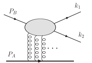
We focus on the two particle production (or dijet production at higher energy) in the case of a dilute system scattering on a dense target, as illustrated in Fig. 1,
| (1) |
where represents the dense target (we shall call it a nucleus in the following), stands for the dilute projectile (such as a photon or a high- parton in a hadron), and are the final state two particles with momenta and , respectively. Let us denote as the light-cone momentum fraction of the parton (or virtual photon) from the incoming projectile , and as the momentum fraction of the gluon from the incoming target. We are interested in the kinematic region where the transverse momentum imbalance between the outgoing particles is much smaller than their individual momenta: where is defined as . This is referred to as the back-to-back correlation limit (the correlation limit) in the following discussions. An important advantage of taking this limit is that we can apply the power counting method to obtain the leading order contribution of where the differential cross section directly depends on the UGDs of the nuclei.
For each individual dijet production process, we employ two independent approaches, namely the TMD approach and the CGC approach222Our formulation of the CGC approach leads to similar intermediate steps as in Ref. Nikolaev:2005qs . However, we treat the -point functions differently by using Wilson lines.. The TMD approach is straightforward and clear in terms of factorization. On the other hand, the CGC approach is commonly used in dealing with small- calculations. It allows to go beyond the correlation limit, which gives a deeper access to the QCD dynamics at small , but this is not the purpose of this paper. In this more general situation, cross sections involve multi-gluon distribution functions, as expected due to parton saturation and multiple scatterings, and therefore there is no -factorization. Except for the most inclusive observables (such as inclusive and semi-inclusive DIS, single-gluon and valence quark production in pA collisions), factorization is only a property of the linear BFKL regime. However taking the correlation limit allows to simplify the dijet production results of the CGC, and to obtain an effective factorization which coincides with that found in the TMD approach.
The Weizsäcker-Williams gluon distribution can be defined following the conventional gluon distribution Collins:1981uw ; Ji:2005nu
| (2) |
where is the gauge field strength tensor with the antisymmetric structure constants for , and
is the gauge link in the adjoint representation with . It contains a transverse gauge link at spatial infinity which is important to make the definition gauge invariant Belitsky:2002sm . These gauge links have to be made non-light-like to regulate the light-cone singularities when gluon radiation contributions are taken into account Collins:1981uw . In the above definition, we assume that the hadron is moving along the direction. The light-cone momenta are defined as . This gluon distribution can also be defined in the fundamental representation Bomhof:2006dp ,
| (3) |
where the gauge link with being reduced to the light-like Wilson line in covariant gauge. It is straightforward to see that represents the final state interactions according to its future integration path to .
By choosing the light-cone gauge with certain boundary condition for the gauge potential ( for the specific case above), we can drop out the gauge link contribution in Eqs. (2) and (3) and find that this gluon distribution has the number density interpretation. Then, it can be calculated from the wave functions or the WW field of the nucleus target McLerran:1993ni ; Kovchegov:1998bi . Within the CGC framework, this distribution can be written in terms of the correlator of four Wilson lines as (see Section II.2),
| (4) |
where the Wilson line is defined as . At small- for a large nucleus, this distribution can be evaluated using the McLerran-Venugopalan model333To obtain this result, it was assumed that the color charge densities in the nucleus obey a Gaussian distribution with variance . It was recently argued that this assumption is inconsistent with the QCD non-linear evolution Dumitru:2010ak , except for two-point functions. McLerran:1993ni
| (5) |
where is the number of colors, is the transverse area of the target nucleus, and is the gluon saturation scale Iancu:2003xm with the color charge density in a large nuclei. We have cross checked this result by directly calculating the gluon distribution function in Eq. (2) following the similar calculation for the quark in Ref. Belitsky:2002sm ; Brodsky:2002ue . The derivation of the WW gluon distribution from its operator definition is provided in Appendix A.1.
The second gluon distribution, the Fourier transform of the dipole cross section, is defined in the fundamental representation444The Fourier transform of the dipole cross section in the adjoint representation is also commonly used, as it enters single gluon production in collisions Kovner:2001vi ; Kovchegov:2001sc ; Marquet:2004xa . In the large- limit, it is related to the convolution of two .
| (6) |
where the gauge link stands for initial state interactions. Thus, the dipole gluon distribution contains both initial and final state interactions in the definition.
and are the gauge links which appear in the quark distributions in the DIS and Drell-Yan process, respectively. It is well-known that there is only final state effect in the DIS, while there is only initial state interaction in the Drell-Yan process. In addition, in processes involving gluons and more complicated partonic structures, more complex gauge links may appear, such as combinations of and Bomhof:2006dp . We will see this in our following calculations especially in dijet production in collisions.
For the second gluon distribution as shown in Eq. (6), the gauge link contribution can not be completely eliminated. In other words, there is no number density interpretation for this gluon distribution. This is also because it contains both initial and final state interaction effects. Due to the gauge link in this gluon distribution from to , naturally this gluon distribution can be related to the color-dipole cross section evaluated from a dipole of size scattering on the nucleus target, and has been calculated in the CGC formalism,
| (7) |
The derivation of this dipole gluon distribution from its operator definition is provided in Appendix A.2.
These two gluon distributions have been intensively investigated in the last few years555There have been an observation that these two UGDs can be related through a mathematical formula where stands for the gluon distribution in the adjoint representation which is derived from a dipole formed by two gluons (e.g., see ref. Kharzeev:2003wz ). However, we believe that this relation is just a mathematical observation without any physics derivation. In addition, we find that it only works for MV model which assumes the local gaussian approximation. This mathematical relation is invalidated beyond the local gaussian approximation. (e.g., see Appendix A.1.) From the above operator definition of these two UGDs, we can see that they are two independent gluon distributions. . In particular, it was found that they
-
•
have the same perturbative behavior. They both scale as at large transverse momentum ;
-
•
however, they differ dramatically at small transverse momentum: whereas .
It will be very important to test these predictions by measuring the quark-antiquark correlation in DIS process and direct photon jet correlation in collisions, since these processes can directly probe these two gluon distributions separately.
The second gluon distribution () depends on the dipole cross section, which appears in various inclusive and semi-inclusive processes. For example, the total cross section (or the structure functions) in DIS, the single inclusive hadron production in DIS and collisions, and the Drell-Yan lepton pair production in collisions, are all depending on this dipole gluon distribution. Tremendous phenomenological analysis have been performed to constrain this gluon distribution from the experimental data.
On the other hand, the first gluon distribution () only appears in few physical processes. Thus, we do not have much constraints on its behavior. The only knowledge comes from model calculations (i.e., the GBW modelGolecBiernat:1998js which provides a good description of all DIS data below x = 0.01). Therefore, it is very crucial to carry out experimental observation of the quark-antiquark jet correlation in DIS process in the planed Electron-Ion collider, which shall provide very important information on this gluon distribution.
Two particle production in collisions are found to depend on both gluon distributions Dominguez:2010xd . In Table I, we summarize the current status for the two gluon distributions probed in high energy processes, where we find that the dipole gluon distribution contributes to most of them, such as inclusive DIS, semi-inclusive DIS(SIDIS) Marquet:2009ca , Drell-Yan (DY) processes, single inclusive hadron production in collisions, photon-jet correlations and dijet in collisions, whereas the WW gluon distribution only appears in the quark-antiquark dijet correlation in DIS and dijet correlations in collisions. It is important to note that our derivations for the two basic processes, where the two distributions can be measured independently (dijet correlations in DIS and photon-jet correlation in collisions), are exact for finite . The large- limit is only necessary for more complicated processes where it allows us to write the new distributions as convolutions of the two basic ones.
| DIS and DY | SIDIS | hadron in | photon-jet in | Dijet in DIS | Dijet in | |
|---|---|---|---|---|---|---|
| (WW) | ||||||
| (dipole) |
In the following sections, we will carry out the detailed derivations for the two-particle correlations in these processes. Quark-antiquark correlation in DIS process will be calculated in Sec.II. Sec.III will be devoted to the direct photon jet correlation in collisions. We will derive the formalism for dijet correlation in collisions in Sec. IV. Summary and further discussions will be given in Sec. V. In all these calculations, we will show the results from both transverse momentum dependent approach and the CGC calculations and we will demonstrate that they are consistent in the correlation limit.
II Dijet production in DIS
Despite the nice physical interpretation, it has been argued that the gluon distribution in Eq. (2) is not directly related to physical observables in the CGC formalism. However, we will show that can be directly probed through the quark-antiquark jet correlation in DIS,
| (8) |
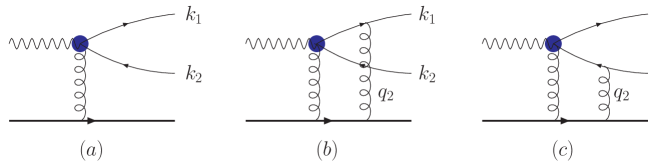
where the incoming (virtual) photon carries momentum , the target nucleus has momentum , and the final state quark and antiquark with momenta and , respectively. Again, we focus on the kinematic region with the correlation limit: . The transverse momenta are defined in the center of mass frame of the virtual photon and the nucleus . The calculations are performed for in the same order of . As we discussed in the above, we take the leading order contribution in the correlation limit: , and neglect all higher order corrections. We plot the typical Feynman diagram for the process of (8) in Fig. 2, where the bubble in the partonic part represents the hard interaction vertex including gluon attachments to both quark and antiquark lines. Fig. 2 (a) is the leading Born diagram whose contributions can be associated with the hard partonic cross section times the gluon distribution from Eq. (2) qvy-short . In high energy scattering with the nucleus target, additional gluon attachments are important and we have to resum these contributions in the large nuclear number limit. Figs. 1(b,c) represent the diagrams contributing at two-gluon exchange order, where the second gluon can attach to either the quark line or the antiquark line. By applying the power counting method in the correlation limit (), we can simplify the scattering amplitudes with the Eikonal approximation qvy-short . For example, Fig. 2 (b) can be reduced to:
| (9) |
where is the gluon momentum, is the color matrix in the fundamental representation and represents the rest of the partonic scattering amplitude with color indices for the two gluons and . Similarly, Fig. 2(c) can be reduced to:
| (10) |
The sum of these two diagrams will be . Because of the unique color index in , we find the effective vertex as,
| (11) |
which corresponds to the first order expansion of the gauge link contribution in the gluon distribution defined in Eq. (2). For all high order contributions, we can follow the procedure outlined in Ref. Belitsky:2002sm ; Bomhof:2006dp to derive the gluon distribution.
In particular, we calculate the differential cross section contributions from the diagrams of Fig. 2, assuming the generic coupling between the exchanged gluons and the nucleus target. The contributions at given order can be reproduced by the hard partonic cross section (given below) multiplying the TMD gluon distribution defined as Eq. (2) at the same order from the similar diagrams. This method is particular useful to identify the gluon distributions involved in the hard scattering processes and will be applied throughout the following calculations.
Of course, to build a rigorous TMD factorization theorem for this process, we have to go beyond the diagrams shown in Fig. 2, and include the real gluon radiation contributions Collins:1981uw ; Ji:2005nu . These diagrams will introduce the large logarithms of , in addition to the small- logarithms . The combination of both effects has not yet been systematically studied in the literature. We hope to address this issue in the future. Moreover, there have been discussions on the power counting method to factorize the gluon distribution from any generic Feynman diagrams, where one has to be extra cautions about the “super-leading-power” contributions (see, for example, Ref. Collins:2008sg ).
From our analysis, we identified the gluon distribution involved in the quark-antiquark jet correlation in DIS process is the first gluon distribution at small-. We want to emphasize that this result is also the unique consequence of non-abelian feature of QCD. For Abelian theory, we can easily find that the final state interactions between the quark and antiquark with the nucleus target cancel out completely. Therefore, there is no final state interaction effects in the similar QED process.
Furthermore, the gauge link in Eq. (3) can be viewed as the sum of all the final state interactions between the nucleus target and the produced quark as shown in Fig. 2 (b). In the meantime, the gauge link in Eq. (3) takes care of the final state interactions between the nucleus target and the produced antiquark as illustrated in Fig. 2 (c). Therefore, following Ref. Bomhof:2006dp , it is straightforward to show that the Weizsäcker-Williams gluon distribution is the relevant gluon distribution in DIS dijet since it correctly resums all the final state interactions.
II.1 TMD-factorization approach to the DIS dijet production
By putting in the hard partonic cross section and especially the correct gluon distribution, namely the WW gluon distribution, which resums all the final state interactions between the pair and the target nucleus, we obtain the following transverse and longitudinal differential cross sections for the quark-antiquark jet correlation in DIS process
| (12) | |||||
| (13) |
where is the momentum fraction of hadron carried by the gluon and is determined by the kinematics, with and being the momentum fractions of the virtual photon carried by the quark and antiquark, respectively. The phase space factor is defined as , and and are rapidities of the two outgoing particles in the lab frame. In terms of the rapidities and the center of mass energy , one can find
| (14) |
In addition, in the correlation limit, one has . The leading order hard partonic cross section reads
| (15) | |||||
| (16) |
with the usually defined partonic Mandelstam variables , , and with and .
Finally, in the correlation limit, one obtains the differential total cross section as follows:
| (17) | |||||
where is defined as and we have substituted the CGC result for the WW gluon distribution in Eq. (5). By taking , we can extend the above result to the case of dijet production in real photon scattering on nuclei. The longitudinal contribution vanishes and the total cross section only contains the transverse part. Therefore, we obtain
| (18) | |||||
For the real photon case, there will be resolved photon contributions which should be taken care separately following that in the dijet production in collisions discussed in Sec. IV below.
II.2 CGC approach to the DIS dijet production
The quark-antiquark jet cross section can also be calculated in the CGC formalism. In this setup the photon splits into a quark-antiquark pair which subsequently undergoes multiple interactions with the nucleus (see Fig. 3). Previous calculations performed under this framework Kovner:2001vi ; Gelis:2002nn have focused mainly on the total cross section or single inclusive gluon production, which are calculations involving a different color structure than the process we are interested in. Here we calculate the cross section in the most general case and then we show how the factorization formula is recovered in the correlation limit.

At the amplitude level the process can be divided into two parts: the splitting wave function of the incoming photon and the multiple scattering factor. It is convenient to write these quantities in transverse coordinate space since in this basis, and in the eikonal approximation, the multiple interaction factor is diagonal. To be consistent with previous CGC calculations in the literature, we choose a frame that the photon is moving along the direction whereas the nuclear target in the direction. When we compare the results to those obtained in the last subsection, we have to keep in mind this difference. However, we note that the differential cross section does not depend on the frame. For a right-moving photon with longitudinal momentum , no transverse momentum, and virtuality , the splitting wave function in transverse coordinate space takes the form,
| (19) | ||||
| (20) |
where again is the momentum fraction of the photon carried by the quark, is the photon polarization, and are the quark and antiquark helicities, the transverse separation of the pair, , and the quarks are assumed to be massless. The heavy quark case will be considered in the next subsection.
The multiple scattering factor is expressed in terms of Wilson lines in the fundamental representation. It can be shown Gelis:2002nn that this interaction term takes the form where and are the transverse positions of the quark and the antiquark, and are their color indices, and the Wilson line is given in terms of the background field by
| (21) |
The gauge field is directly related to the color charge density of the nucleus which will be averaged over the nuclear wave function at the level of the cross section. The way the color indices are contracted in the scattering factor is due to the fact that the pair is initially in a singlet state but no assumptions are made about the final state. The color indices and will be summed over independently also at the cross section level.
With the pieces described above we can write down an explicit formula for the differential cross section for dijet production. After averaging over the photon’s polarization and summing over the quark and antiquark helicities and colors we obtain,
| (22) | |||||
where the two- and four-point functions are defined as
| (23) | |||
| (24) |
The notation is used for the CGC average of the color charges over the nuclear wave function where is the smallest fraction of longitudinal momentum probed, and is determined by the kinematics.
Notice that the transverse coordinates of the quark and antiquark in the amplitude (unprimed coordinates) are different from the coordinates in the complex conjugate amplitude (primed coordinates) since the two final momenta are not integrated over. This is a very important feature of our calculation that, to our knowledge, does not appear in previous CGC calculations of DIS in nuclei. It allows for a different color structure and in particular it is responsible for the appearance of the 4-point function which cannot be expressed in terms of 2-point functions, even in the large limit (see Appendix B.2 for an explicit evaluation of the medium average).
In order to compare with the TMD-factorization result discussed in the previous section, we need to consider the relevant kinematic region, in particular in the correlation limit of Eq. (22). For convenience, we introduce the transverse coordinate variables: and , and similarly for the primed coordinates. The respective conjugate momenta are and , and therefore the correlation limit can be taken by assuming and are small and then expanding the integrand with respect to these two variables before performing the Fourier transform.
Let us focus on the multiple scattering factor first. By using the following identities,
| (25) | |||||
| (26) |
it is easy to see that terms from the expansion of cancel the other terms in (22). After applying
we can show that the lowest order contribution in and to the scattering factor can be written as
| (27) |
Taking into account the path ordering of the Wilson lines, we have the following formula for their derivatives,
| (28) |
where . We notice that is part of the gauge invariant field strength tensor 666The other part of the the field strength tensor shall come from the transverse component of the Wilson lines as the gauge invariance of QCD requires. When the gauge is used the only non-zero component of the gauge field is Gelis:2005pt and the transverse parts drop out of the equations, giving a simpler form of the equations.. Therefore, the above correlator can be written in terms of gauge invariant matrix element,
| (29) |
Performing the and integration in (22) after the expansion of the multiple scattering term, we find an explicit formula for the differential cross section in the desired kinematic region,
| (30) | |||||
| (31) | |||||
These results are to be compared to the factorized results in Eq. (12,13). The hard cross section factor in (12) is recovered by noticing that in the kinematic region we are considering the Mandelstam variables are given by , , and . To recover the gluon distribution function as written in Eq. (3) it is necessary to account for the different normalizations used to calculate the average of Wilson lines above. In Eq. (3) the average is calculated with a definite momentum (and therefore translational invariant) hadronic state which is relativistically normalized to , while the average in Eqs. (30) and (31) is taken over the CGC wave function and is normalized such that . Using translational invariance Eq. (3) can be written as
| (32) | |||||
It is easy to see that the discrepancy between normalizations is accounted for by the replacement , giving complete agreement between the CGC approach and the factorized form in the small- region.
In the end of this subsection, we would like to compare the dijet production process in DIS to the inclusive and semi-inclusive DIS. As shown above, we derive that the dijet production cross section in DIS is proportional to the WW gluon distribution in the correlation limit. On the other hand, it is well-known that inclusive and semi-inclusive DIS involves the dipole cross section instead Marquet:2009ca , which can be related to the second gluon distribution. This might look confusing at first sight, so let us take a closer look at Eq. (22). If one integrates over one of the outgoing momenta, say , one can easily see that the corresponding coordinates in the amplitude and conjugate amplitude are identified () and, therefore, the four-point function collapses to a two-point function . As a result, The SIDIS and inclusive DIS cross section only depend on two-point functions, thus they only involve the dipole gluon distribution. Now we can see the unique feature of the dijet production process in DIS. By keeping the momenta of the quark and antiquark unintegrated, we can keep the full color structure of the four-point function which eventually leads to the WW gluon distribution in the correlation limit. Therefore, measuring the dijet production cross sections or dihadron correlations in DIS at future experimental facilities like EIC or LHeC would give us a first direct and unique opportunity to probe and understand the Weizsäcker-Williams gluon distribution.
II.3 Heavy quark production in DIS dijet
In order to expand our calculation and include the possibility of charm and bottom production, we now consider the finite quark mass case. From the TMD point of view, having massive quarks modifies the hard cross sections while the parton distributions remain the same. The new leading order hard partonic cross sections read
| (33) | |||||
| (34) |
where , , and with and .
In terms of the CGC approach, one needs to modify the dipole splitting wave functions as follows:
| (35) | ||||
| (36) |
Following the same procedure, it is easy to show that again both approaches agree in the correlation limit for heavy quark production. By setting , one can get the results for the heavy quark production in real photon-nucleus scattering.
III Direct-photon jet in collisions
Now let us turn our attention to the second gluon distribution. In this context, the simplest process where we can access this distribution is the direct photon-quark jet correlation in collisions,
| (37) |
where the incoming quark carries momentum , and nucleus target with momentum , and outgoing photon and quark with momenta and , respectively. The analysis of this process follows that for the quark-antiquark jet correlation in DIS process in the previous section.
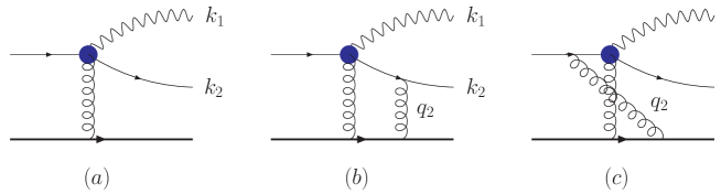
We plot the relevant diagrams in Fig. 4(a,b,c), again for the leading one gluon exchange and two gluon exchanges. Similarly, the two gluon exchange contributions can be summarized as777There is a misprint, which we have corrected below in the eq.(38), in the Eq.(11) of the short summary Dominguez:2010xd of this paper.)
| (38) |
where the plus sign comes from the fact that the second gluon attaches to the quark line in the initial and final states. Since there is no color structure corresponding to Eq. (38), we can only express it in the fundamental representation. Following Ref. Bomhof:2006dp , we find that the gluon distribution in this process can be written as
| (39) |
where the gauge link resums the initial state interactions between the incoming quark and the target nucleus. On the other hand, the gauge link represents the final state interactions between the outgoing quark and the target nucleus. This gluon distribution can also be calculated in the CGC formalism where it is found to be
| (40) |
with the normalized unintegrated gluon distribution . Therefore, by plugging in the appropriate gluon distribution, namely the dipole gluon distribution, which resums both the initial and final state interactions, one can write the differential cross section of (37) as888Here we assume that one can employ the collinear factorization for the integrated quark density or gluon density inside the dilute proton at large , although the proof of this assumption is omitted throughout this paper. We will leave this study for future work.
| (41) |
where is the momentum fraction of the projectile nucleon carried by the quark, is the integrated quark distribution. Because we are taking large nuclear number limit, the intrinsic transverse momentum associated with it can be neglected compared to that from the gluon distribution of nucleus. The hard partonic cross section is given by
| (42) |
Inserting Eqs. (40) and (42) in Eq. (41), one gets
| (43) |
where we have expressed the Mandelstam variables in terms of and : , and . The momentum fraction of the incoming quark carried by the outgoing photon is defined as
| (44) |
where and are rapidities of the photon and outgoing quark in the Lab frame.
The current running RHIC and LHC experiments shall provide us some information on the dipole gluon distribution by measuring direct photon-quark jet correlation in collisions.
III.1 CGC approach to the direct photon-jet production in collisions
This process was already considered in the CGC framework in Gelis:2002ki where the calculation was performed entirely in momentum space. In order to compare with the result from the previous section and illustrate why a different distribution should be used, we will derive the corresponding cross section following the same procedure as the previous section by showing the splitting wave function and the multiple scattering factor in transverse coordinate space. Our result is consistent with Gelis:2002ki .
Let us consider the partonic level process . For a right-moving massless quark, with initial longitudinal momentum and no transverse momentum, the splitting wave function in transverse coordinate space is given by
| (45) |
where again is the photon polarization, are helicities for the incoming and outgoing quarks, and is the momentum fraction of the incoming quark carried by the photon. To account for the multiple scatterings in this process we have to consider interactions both before and after the splitting. If the transverse coordinates of the quark and photon in the final state are and respectively, then the multiple scattering factor in the amplitude takes the form .
After summing over final polarization, helicity and color, and averaging over initial helicity and color, we find the following expression for the partonic level cross section (see Fig. 5).
| (46) | |||||

Notice that the color structure is simpler than in the DIS case. There is no four-point function and all the terms in the multiple scattering factor can be expressed in terms of the color dipole cross section . By changing the variables on each of the terms of the scattering factor to and either or , and similarly for the primed coordinates, the cross section above can be written as
| (47) | |||||
where .
From the above expression it is easy to see that performing the and integrations reduces to taking the Fourier transform of the splitting wave function with different values of the momentum variable for each term. Clearly, the Fourier transform of the dipole cross section factors out giving the gluon distribution we found from the TMD-factorized form. Using collinear approximation for the proton projectile we find our final result for the cross section of the desired process.
| (48) |
This result agrees with the factorized result (41) in the correlation limit . To make more clear the relation between the distribution in Eq. (6) and the result above notice that the factor can be brought inside the integral as derivatives of the exponential factor with respect to and . Using integration by parts and the derivation formula for Wilson lines it is easy to show that the cross section takes the form
| (49) |
Taking into account the same considerations about different normalizations of the averaging procedures as in the DIS case, it is easy to see that the two expressions for agree in the small- region.
IV Dijet production in collisions
Dijet production in collisions receive contributions from several channels such as , and . For convenience, we define the following common variables as in the last two sections,
| (50) |
where and are momenta, and and are rapidities for the two outgoing particles, is the momentum fraction of the projectile nucleon carried by the incoming parton, is the momentum fraction of the target nucleus carried by the gluon, respectively. Taking into account that the quark distribution functions are dominant at large- and the gluon distribution functions are dominant at low-, it comes as no surprise the fact that different channels are relevant in different kinematic regions. At RHIC energies, the low - region is only accessible in events where the two jets are produced in the forward rapidity region of the projectile. Under those conditions we have and , and therefore quark initiated processes dominate ( channel).
The higher energies available at LHC will allow to explore more thoroughly the low- regime in the target nucleus as well as in the projectile(see e.g., in a recent studyDeak:2010gk ). Under these circumstances, and in particular at central rapidities at the LHC, it is possible to have processes with both and small where the dominant channels are and .
Let us first take the partonic channel as an example and calculate the dijet production cross section. Then it is straightforward to generalize the calculation to the other partonic channels and .
IV.1 TMD-factorization approach
IV.1.1 The channel
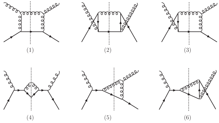
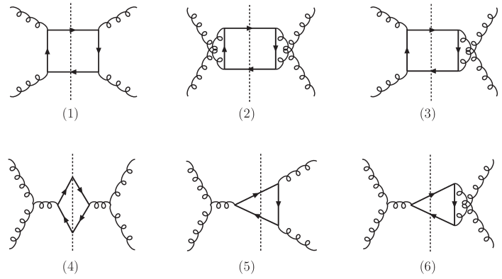
The calculations follow the previous examples. However, there are several different Feynman graphs contributing to the production of in the final state, as shown in Fig. 6. In addition, they have different color structures. Therefore, we need to compute the hard factors and the associated initial/final state interaction phases separately. In the end, we will sum their contributions together to obtain the final result.
It is straightforward to obtain the hard cross section contributions from each diagram in Fig. 6 for the process, and have been calculated in Ref. qvy-short . We list these results in Table 2 with the same notations, where is the partonic hard factor and is the associated color factor. In the calculations, in order to apply the eikonal approximation when multiple gluon interactions are formulated, we have chosen the physical polarizations for the outgoing gluon. However, the final result for the differential cross section does not depend on this choice.
| (1) | (2) | (3) | (4) | (5) | (6) | |
|---|---|---|---|---|---|---|
As a consistency check, we can easily reproduce the known results for the total hard cross section by summing all the graphs in Fig. 6 and explicitly taking ,
| (51) | |||||
Since the graphs in Fig. 6 have different color structure, the gluon distributions associated with those graphs have different gauge links according to Ref. Bomhof:2006dp . Therefore, the corresponding gluon distributions in coordinate space are found as follows:
| (52) | |||||
| (53) | |||||
| (54) | |||||
| (55) |
where emerges as a Wilson loop. Now we are ready to combine all the channels together. As mentioned in the introduction, the distributions above will be factorizable in terms of convolutions of the two basic distributions from the previous sections. Anticipating this result, we consider only the leading contribution in . Noting that graph (6) in Fig 6 does not contribute in the large- limit, one can find
| (56) |
with
| (57) | |||||
| (58) |
In the large- limit, it is straightforward to find that only graphs (1), (2) and (3) in Fig. 6 ( and channels together with their cross diagrams) contribute to and only graphs (1), (4) and (5) ( and channels together with their cross diagrams) contribute to . By using in the large- limit, one obtains
| (59) | |||||
| (60) |
We note that although the individual diagram’s contribution to the above two hard factors depends on the polarization we choose for the outgoing gluon, the final results for the hard factors do not depend on this choice. This means the combination of Feynman graphs according to the relevant color structure is gauge invariant. Similar conclusion has also been obtained for the spin related observables calculated in Refs. Bomhof:2006dp ; qvy-short .
Since one has , and in the correlation limit, Eq. (56) leads to the following cross section for dijet production in collisions
| (61) | |||||
where is the integrated quark distribution for the proton projectile.
IV.1.2 The channel
| (1) | (2) | (3) | (4) | (5) | (6) | |
|---|---|---|---|---|---|---|
Following the same procedure illustrated in the channel, we can calculate the dijet production cross section from the channel. First of all, we compute the color factors and hard factors for each graph in Fig. 7 and list them in Table 3. Then, we plug in the appropriate gluon distributions999We have simplified these gluon distributions by using large- limit and the fact that they are real in the CGC formalism. as found in Ref. Bomhof:2006dp .
| (62) | |||||
| (63) | |||||
| (64) | |||||
Combining all the channels in the large limit, we can find
| (65) |
with
| (66) | |||||
| (67) |
and
| (68) | |||||
| (69) |
where is the integrated gluon distribution in the proton projectile.
IV.1.3 The channel
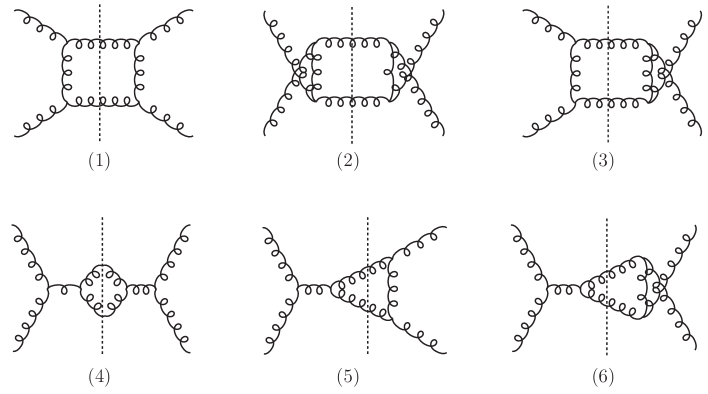
| h | ||
|---|---|---|
| (1) | ||
| (2) | ||
| (3) | ||
| (4) | ||
| (5) | ||
| (6) |
Similarly, the color factors and hard factors for all the graphs plotted in Fig. 8 have been calculated and listed in Table 4. Combining these factors with the corresponding gluon distributions, taking into account the appropriate gauge links Bomhof:2006dp , we arrive at
| (70) | |||||
| (71) | |||||
| (72) | |||||
Summing over all the channels in the large- limit, we can obtain
| (73) |
where have been defined in Eqs. (66,67) and is defined as
| (74) |
The hard factors are found as
| (75) |
Using the mean field approximation Xiao:2010sp , we can simplify the gluon distributions and find the total dijet production cross section which includes the , and channels as follows
| (76) | |||||
where again and are integrated quark and gluon distributions from the projectile nucleon. We have included a statistical factor of in Eq. (76) for the channel due to the identical final state. The various gluon distributions of nucleus are defined as
| (77) |
where represents the convolution in momentum space: . These expressions follow directly from Eqs. (57), (58), (66), (67), (74) and the assumption that in the large- limit the expectation values involved in these equations can be factored as products of expectation values of the traces within. Clearly, this process depends on both UGDs in a complicated way, and the naive TMD-factorization does not hold.
IV.2 CGC Calculations
IV.2.1

This process is studied in detail in Refs. JalilianMarian:2004da ; Marquet:2007vb , and in particular Ref. Marquet:2007vb is close to the approach we have followed in this paper, where an explicit formula analogous to the ones cited here for DIS and photon emission is given. We take as starting point Eq. (24) in Ref. Marquet:2007vb which in our notation takes the form (see Fig. 9)
| (78) | |||||
where
| (79) | ||||
| (80) |
and is a Wilson line in the adjoint representation. In the correlators above, Wilson lines in the fundamental representation appear when considering the multiple interaction of a quark with the nucleus and Wilson lines in the adjoint representation appear when considering multiple interactions of a gluon with the nucleus. Clearly, the term represents the case where interactions occur after the splitting both in the amplitude and in the conjugate amplitude, the terms represent the interference terms, and the term represent interactions before the splitting only.
This formula for the cross section has the same structure as Eqs. (22) and (47). The splitting wave function is the same as in the photon emission case (Eq. (45)). The only difference in the emission vertex is a color matrix which is included as part of the multiple scattering factor (therefore confining the color algebra to just the multiple scattering factor). Using Fierz identities, the terms appearing in the multiple scattering factor above can be written in terms of fundamental Wilson lines only as
| (81) | ||||
| (82) |
Some of the correlators appearing in the expressions above are familiar or have been calculated in the literature before. The 4-point function in is different from the one appearing in the DIS case but it has been studied and calculated in a model with Gaussian distribution of sources in Dominguez:2008aa . The 6-point function appearing in presents a more difficult challenge even with only four independent coordinates. In order to deal with this difficulty, it is convenient to address the problem in the large- limit where correlators of products of traces are evaluated as product of correlators of traces. Specifically, for the correlators above we get
| (83) | ||||
| (84) | ||||
| (85) | ||||
| (86) |
Note that in the large- limit, the 6-point function is related to the 4-point function that appeared in the DIS dijet case. In Appendix B.2, we point out that the result of Marquet:2007vb for the 6-point function misses the inelastic part of .
To enforce the correlation limit we follow the procedure used in the DIS case. From the structure of the terms in the multiple scattering factor, we can see that the same kind of cancellations will occur and the final result will be the sum of the lowest order non-vanishing terms from the expansion of . Moreover, since there is no linear term in the expansion of , the lowest non-vanishing terms come separately from the factor and the in the same fashion as in the previous calculations for DIS and photon emission. With the previous considerations in mind, it is easy to see that the final result takes the form
| (87) |
Taking into account the difference between the normalizations, it is straightforward to see that the result above agrees with the factorized formula (61).

In order to bring some insight to the relation between the processes considered so far, and how the different distributions come in for this particular channel, it is useful to consider the graphical representation of the large- limit used to factorize the correlators of Wilson lines. In the large- limit, a gluon line can be effectively considered as a quark-antiquark pair. Forgetting about the multiple interactions for the moment, and focusing primarily in the color flow of the process, we see that in the large- limit the process takes the form depicted in Fig. 10. The system splits into two separate pieces, a quark line in the lower part of the diagram which resembles the photon emission process, and a loop in the upper part of the diagram which has the same color structure as the DIS dijet case. Interactions involving both parts of the process are -suppressed, so it comes as no surprise that the final result can be written as two separate pieces each involving the respective distributions found for DIS and photon emission.
The fact that one of the terms in the final result involves only one of the distributions while the other involves a convolution of two factors can also be understood in a simple way from the previous considerations. The enforcement of the correlation limit is schematically the same as singling out one hard scattering in the process and then taking for the rest of the interactions. When the hard scattering occurs on the lower part of the diagram in Fig. 10, the quark-antiquark pair in the upper part does not interact by color transparency () and therefore there is no trace of it in the first term of the factorized expression. When the hard scattering occurs in the upper part of the diagram in Fig. 10, the quark in the lower part still interacts with the nucleus (and exchanges transverse momentum) and therefore has to be included in the form of a dipole cross section.
IV.2.2
Following the same strategy from previous sections, we start with the partonic level formula for the cross section built from the splitting wave function and the multiple scattering factor. In this particular case it takes the following form,
| (88) | |||||
where is given by (82) and
| (89) | ||||
| (90) |
and the splitting wave function is the same as in the DIS case with . Notice this cross section is down by a factor of as compared to the case. This is due to the averaging over the incoming particle which amounts for a factor of for gluons instead of the factor of for quarks.
All the correlators above have been previously studied in the literature and explicit expressions for a Gaussian distribution of charges have been found. The only new ingredient that has not been considered in previous sections is which was thoroughly studied in Blaizot:2004wv . Following the procedure from the previous section, let us express the correlators defined above in terms of fundamental Wilson lines only by means of Fierz identities.
| (91) | ||||
| (92) |
We take the large- limit in order to be able to compare with the results from the previous section and relate the cross section to the gluon distributions defined before. Under this approximation, the correlators above can be expressed entirely in terms of 2-point functions.
| (93) | ||||
| (94) |
This way of factorizing the correlators and the fact that the 4-point function is absent suggests that this process is related to the distribution given by the Fourier transform of the dipole cross section only. With this consideration in mind, we Fourier transform all the factors and perform the usual change of variables and (and similarly for the primed coordinates) and obtain
| (95) | |||||
As in the photon emission case, the and integrations reduce to calculate the Fourier transform of the splitting wave function with different momentum variables for each of the terms. The and integrations give a -function relating the momentum variables of the two distributions and a factor of the total transverse area. As in previous cases, we use collinear factorization for the incoming parton from the proton projectile and obtain
| (96) |
In the correlation limit, the denominator of the last fraction above becomes just . From this expression it is clear that the distributions involved will be written as a convolution of two factors involving the Fourier transform of the dipole cross section. To notice how this equation above agrees with the factorized form in (65), expand the numerator and write the momentum factors as derivatives with respect to transverse coordinates of the dipole cross sections inside the definition of as was explained for the case of photon emission. There is a subtlety concerning the relative signs of the different terms when this identification is made. In order to find a complete agreement between the formula above and the factorized formula from the TMD formalism, it is necessary to write the two factors as Fourier transforms of Wilson loops in opposite directions (one of them in terms of and the other in terms of ). Because of this, and enter with opposite signs when expressed as derivatives of the Wilson loops. This sign is not visible in the terms with or but it changes the sign of the cross term, giving complete agreement with the factorized expression.


As done for the previous channel, let us consider the graphical representation of this channel in the large- limit in Fig. 11. After replacing the gluon line with a quark-antiquark pair we are left with two independent fermion lines which scatter separately with the nucleus. Each of them resembles the photon emission case and therefore we expect, even before performing the calculation, to obtain a convolution of two Fourier transforms of the dipole cross section. In the correlation limit, the two terms in (65) have a simple explanation in terms of a hard scattering. The first term accounts for the cases where the hard scattering involves only one of the two quark lines, while the second term is an interference term when the large momentum transfer involves the two participants.
This channel had already been considered in Blaizot:2004wv where, due to the choice of gauge, the separation of the amplitude in terms of splitting function and multiple scattering terms is not visible. It is possible to show our expressions above are consistent with their results when expressed in the same set of coordinates and momentum variables.
IV.2.3 ggg
In order to study the partonic process , we need to derive the splitting function first. It can be written in momentum space as
| (97) |
where is just the three-gluon vertex with the coupling and color factor factorized out. This can be written as
| (98) |
Here represents the polarization vector for gluon with four momentum . It is straightforward to find that
| (99) |
After summing over all polarizations, the squared splitting function in transverse coordinate space reads
| (100) |
Now let us turn our attention to the multiple scattering terms. Since all the particles involved in the process are gluons, all terms contain only Wilson lines in the adjoint representation. In the following we give the explicit forms of the scattering terms with their respective large- expressions in terms of fundamental Wilson lines.
| (101) |
| (102) | |||||
| (103) | |||||
| (104) |
The correlation limit is applied by following the procedure developed in the DIS case and reproduced in the channel. By inspection of the multiple scattering terms above, it is easy to see that the same kind of cancelations occur for this channel. Since the lowest order terms left after the various cancelations come from the first of the scattering terms, it is easy to see that the final result will involve combinations of one WW distribution and two Fourier transforms of the dipole cross section. After some algebra we arrive at
| (105) | |||||
which is straightforward to compare to the factorized expression in (73).

This structure could have been anticipated by looking at the graphical representation of this process in the large- limit shown in Fig. 12. In terms of the hard scattering picture used in previous sections the structure of the expression above is consistent with previous results. The first and third term look exactly the same as the two terms in the case and they correspond to the case in which the hard scattering does not involve the inner loop in Fig. 12. The second term corresponds to the case where the hard scattering occurs in the inner loop. It has the same structure as one of the terms found in the case with an additional convolution associated to the extra quark line in the top of the diagram.
V Conclusion
In this paper, we have studied and established an effective -factorization for dijet production at small- in dilute-dense collisions. Although -dependent parton distributions are different in different processes, they can be calculated and related to each other. We found that there are two fundamental unintegrated gluon distributions, namely, and , at small . Although other different gluon distributions appear in many different dijet production processes, one can compute them and find that they are related to these two fundamental gluon distributions in the large limit. In terms of the CGC framework, this means that the two- and four-point functions are enough to compute any dijet cross section, in the small momentum imbalance limit. In addition, there is similar conclusion for the quark distributions at small Xiao:2010sp . By doing so, we can restore the predictive power of the theory.
Therefore, as part of the conclusion, we would like to summarize the empirical rules in the large- limit101010Note that one does not need to take the large limit in the calculation of and in DIS dijet and photon-jet in pA collisions, respectively. However, the large limit is essential in order to eliminate other non-universal distributions or correlators in other different dijet channels, i.e., , and in pA collisions. in this effective -factorization for dilute-dense system as follows:
-
•
The cross section can be still separated into the products of the hard parts and parton distributions;
-
•
The hard factors should be calculated separately for each individual graph since the parton distribution associated with each graph may be different;
- •
-
•
Quark lines always have interactions with the dense target which contribute or to the gluon distribution. However, the color singlet quark loop may or may not interact with the dense target due to its peculiar color structure. If the quark loop participates the interaction, it contributes to the gluon distribution.
-
•
If there are multiple objects involved in the soft interaction, the resulting gluon distribution can be written in terms of convolutions of all contributions in momentum space. For quark distributions in the dense target, there are similar rules which can be found in Ref. Xiao:2010sp .
Using the above rules and calculating the coefficients of gluon distributions as illustrated in Ref. Bomhof:2006dp , it is then straightforward to write down cross sections in terms of products of hard parts and parton distributions as illustrated in the context of this paper.
There have been ambiguities regarding the unintegrated gluon distributions for more than a decade. In this paper, we resolve this decade-long puzzle through explicit operator definitions and propose measurements in physical processes which probe the distributions directly. In particular, we find that quark-antiquark correlation in DIS collisions can probe the Weizsäcker-Williams gluon distribution formulated in CGC many years ago.
It is well-known that in the color dipole approach, the cross sections of inclusive DIS and SIDIS Marquet:2009ca at small- are proportional to the dipole cross section. Since the dipole cross section can be written as Fourier transform of the normalized gluon distribution , we can study the unintegrated gluon distribution of nuclei through inclusive DIS and SIDIS at EIC. Moreover, using DIS dijet (dihadron) processes at EIC in the correlation limit, we can directly probe the Weizsäcker-Williams gluon distribution which is the distribution that actually counts the number of gluons in the nuclear wave function. This would give us the golden opportunity to access the saturated WW gluon distribution which has been studied for many years.
Recently, both STAR and PHENIX Collaborations have published experimental results on di-hadron correlations in collisions, where a strong back-to-back de-correlation of the two hadrons was found in the forward rapidity region of the deuteron rhic-data . These results have stimulated a number of theoretical calculations in the CGC formalism, where different assumptions have been made in the formulations Albacete:2010pg ; Tuchin:2009nf , though not the correlation limit we had to use in the present study. In particular, the numerical evaluation in Ref. Marquet:2007vb ; Albacete:2010pg only contains the first term in the channel in Eq.(B22). The second term, as well as other missing terms due to the use of a Gaussian approximation Dumitru:2010ak , are equally important and should be taken into account to interpret the STAR data. In addition, we also present the first CGC calculations on the and channels in collisions. Although these channels are subdominant in the forward dijet productions, they are important in the central rapidity region.
At RHIC and LHC, by measuring the direct photon-jet correlation in collisions, one can gain direct information about the dipole unintegrated gluon distribution . Furthermore, by investigating the dijet (quark-gluon or gluon-gluon jet) production in the correlation limit, one can test the universality of gluon distributions, and begin to see the convolutions of these two unintegrated gluon distributions. Using dijet production with more general kinematics, one can even probe deeper the small- QCD dynamics, as multi-gluon distributions become crucial.
Acknowledgements.
We thank Al Mueller for stimulating discussions and critical reading of the manuscript. We thank Alberto Accardi, Emil Avsar, Markus Diehl, Volker Koch, Larry McLerran, Stephane Munier, Jianwei Qiu, Anna Stasto, Raju Venugopalan and Xin-Nian Wang for helpful conversations. This work was supported in part by the U.S. Department of Energy under the contracts DE-AC02-05CH11231 and DOE OJI grant No. DE - SC0002145. We are grateful to RIKEN, Brookhaven National Laboratory and the U.S. Department of Energy (contract number DE-AC02-98CH10886) for providing the facilities essential for the completion of this work. We also thank the Institute for Nuclear Theory at the University of Washington for its hospitality and the Department of Energy for partial support during the completion of this work.Appendix A Derivation of two gluon distributions
A.1 The Weizsäcker-Williams gluon distribution
Let us focus on the Weizsäcker-Williams gluon distribution first. Here we provide a derivation of this gluon distribution from its operator definition, together with the gauge links for a large nucleus, by using the McLerran-Venugopalan model. According to its definition
| (106) |
with . The definition above is gauge invariant. However, in order to simplify the calculation, we have chosen to use covariant gauge. Thus, it is then easy to write it as
| (107) | |||||
where now is in the adjoint representation. Following Belitsky et al Belitsky:2002sm , we can insert a complete set of one particle intermediate states. Notice that for the quark distribution at small-, we need to have two particle intermediate states due to the antiquark spectator. Therefore, the gluon distribution reads
| (108) |
where we introduced the amplitude
| (109) |
This amplitude then takes the form
| (110) |
By plugging in everything into the definition, we find
| (111) |
Let us define as the Fourier transform of . Like what we have done for the quark distributions Xiao:2010sp , we can compute the diagrammatic contributions to order by order and resum it in coordinate space which gives
| (112) |
where
| (113) |
with being the adjoint color matrix. Eventually, one should be able to write
| (114) |
In arriving to the expression above, we have put in a normalization factor of which comes from . In the following, we need to average the above expression with a gaussian distribution of color charges as proposed in CGC. Therefore
| (115) | |||||
Assuming a Gaussian distribution of sources, it is easy to prove that
| (116) | |||||
| (117) |
by using the fact that (Note that is anti-symmetric. See Iancu:2002xk for more details). Therefore, we have
| (118) | |||||
The different factors in the integral above can all be written in terms of a single function when a Gaussian distribution of sources is used. Let
| (119) |
In terms of , Eq. (118) takes the form
| (120) |
In particular, for the McLerran-Venugopalan model, the function can be evaluated explicitly giving the well-known result
| (121) |
where is the gluon saturation scale.
A.2 The dipole gluon distribution
According to its definition
| (122) |
with and . Here we have chosen the covariant gauge to do the calculation. Thus, one gets
| (123) | |||||
By inserting the intermediate state and replacing the by the ensemble average , we get
| (124) |
with
| (125) |
and
| (126) |
In CGC, we can find that, in covariant gauge, the only non-trivial field strength is d. Therefore, if we write
| (127) | |||||
| (128) |
we can easily see that In the above derivation, we have to assume that . This can be justified by noting that is integrated from to with being the longitudinal width of the nucleus. For small with small , we have .
Eventually, one gets
| (129) | |||||
| (130) |
where and d. Here the saturation scale is obtained from the fundamental representation and it is usually called quark saturation momentum.
Appendix B Evaluations of Correlators
Here in this section, we summarize the evaluation of the correlators in CGC used above in the main context of the paper.
B.1 The evaluation of two point functions and
First of all, as derived in Ref. Gelis:2001da , for an arbitrary single Wilson line (start at and end at ) , one can get
| (131) |
Using this result, it is easy to derive that
| (132) |
The derivation is based on time ordering of and pairing of two adjacent operators.
Furthermore, for two infinite Wilson lines of different transverse position, one gets
| (133) | |||||
where stands for the cut-off in the integral. Thus, usually one writes with .
Now we are ready to evaluate and show that it is the same as the correlator of two infinite Wilson lines. According to the definition, one can easily find that
| (134) | |||||
| (135) |
where we have used Eq. (132). Therefore, one can easily relate to through Fourier transform.
B.2 Evaluation of the 4-point function with a Gaussian distribution of sources
The derivation presented here follows closely the method presented in Blaizot:2004wv and used also in Dominguez:2008aa where other 4-point functions have been calculated. For the sake of completeness and to make the presentation self-contained we will briefly review how to calculate the 4-point function for a Gaussian distribution of charges. Details of the general procedure are given in Blaizot:2004wv .
The nuclear average of a function of the gauge field is defined by
| (136) |
where the color charge and the gauge field are related by
| (137) |
and is the density of color charges at a given . This Gaussian distribution allows us to express any correlator in terms of the elementary correlator of two color charges
| (138) |
In order to do this, the Wilson lines must be expanded in terms of and then apply Wick’s theorem. The Wilson lines are naturally expanded in terms of the gauge field and not the color charge density, therefore it is useful to express the elementary correlator (138) in terms of the gauge field.
| (139) |
with given in terms of the two-dimensional massless propagator ,
| (140) |
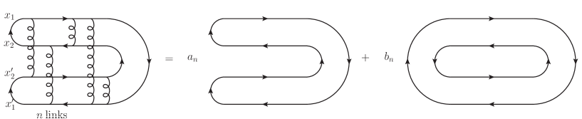
This correlation between two fields has the color structure of a gluon link. This, together with the locality of the correlator in the variable, allows for a graphical representation of each of the terms of the expansion of the Wilson lines. For the particular color structure of the 4-point function we are interested in diagrams which look like the left hand side of Fig. 13. One kind of contribution from these diagrams that is easy to evaluate is the contribution from links with both ends attached to the same line. For a Wilson line at a transverse coordinate this kind of link gives a factor of , it has a color singlet structure and therefore factors out in the evaluation of any specific diagram. When multiple insertions of these particular links are taken into account they can be resummed into the factor
| (141) |
where the contributions from the four Wilson lines involved in the correlator have been included. After factoring out the so-called tadpole contributions we are left with diagrams in which all gluon links connect different Wilson lines. The strategy to evaluate this diagrams is to include the proper factors for each of the gluon links and to resolve the color structure by means of the Fierz identity . The resummation then is not a trivial task since each diagram will end up being written as a linear combination of the two topologies shown in the right hand side of Fig. 13. As shown in Blaizot:2004wv this difficulty can be overcome by grouping diagrams according to the number of gluon links and then using an inductive procedure to find the value of the th term in the series. By explicitly resolving the th link and using the notation in Fig. 13 we have,
| (142) |
where the matrix is given by all the different ways in which the th link can be attached,
| (143) |
with . It is easy to solve this recursion relation taking into account the initial condition . Formally, the solution reads
| (144) |
In order to find an explicit solution we have to find the eigenvalues and eigenvectors of . The solution then takes the form
| (145) |
with
| (146) | |||
| (147) | |||
| (148) |
With this result we can now easily resum the contribution from all the diagrams. The 4-point function is then given by
| (149) |
When written in terms of the eigenvalues above this expression can be resummed into
| (150) |
Using the explicit values shown above, this expression takes the form
| (151) |
with .
Taking the large- limit of this result we find a much simpler expression,
| (152) |
Note that even this large- result can not be expressed as a product of 2-point functions. The two terms appearing above have a simple interpretation in terms of multiple scatterings that allows us to label the first term as the elastic part and the second term as the inelastic part (see JalilianMarian:2004da where the same scattering factor appears in the context of two-gluon production). Taking into account that the Gaussian distribution of sources is equivalent to the two gluon exchange approximation with independent scattering centers, it is easy to see that the first term is what you would expect if only interactions that don’t break up nucleons in the nucleus were allowed. In that scenario the quark-antiquark pair is always on a singlet state and the interaction factor can be written as the product of the interaction term for a dipole in the amplitude times an interaction term for the dipole in the conjugate amplitude. The inelastic part takes into account all the interactions were at least one of the nucleons is broken apart, in which case the quark-antiquark pair goes from a singlet state to an octet state. In the large- limit transitions from the octet state to the singlet state are suppressed and therefore the pair remains in the octet state for the rest of the interaction with the nucleus.
References
- (1) D. Boer and W. Vogelsang, Phys. Rev. D 69, 094025 (2004).
- (2) C. J. Bomhof, P. J. Mulders and F. Pijlman, Eur. Phys. J. C 47, 147 (2006).
- (3) J. W. Qiu, W. Vogelsang and F. Yuan, Phys. Lett. B 650, 373 (2007); Phys. Rev. D 76, 074029 (2007).
- (4) J. Collins and J. W. Qiu, Phys. Rev. D 75, 114014 (2007).
- (5) W. Vogelsang and F. Yuan, Phys. Rev. D 76, 094013 (2007); J. Collins, arXiv:0708.4410 [hep-ph].
- (6) T. C. Rogers and P. J. Mulders, Phys. Rev. D 81, 094006 (2010).
- (7) B. W. Xiao and F. Yuan, Phys. Rev. Lett. 105, 062001 (2010); arXiv:1008.4432 [hep-ph].
- (8) L. V. Gribov, E. M. Levin and M. G. Ryskin, Phys. Rept. 100, 1 (1983).
- (9) A. H. Mueller and J. w. Qiu, Nucl. Phys. B 268, 427 (1986).
- (10) L. D. McLerran and R. Venugopalan, Phys. Rev. D 49, 2233 (1994); Phys. Rev. D 49, 3352 (1994).
- (11) E. Iancu, A. Leonidov and L. McLerran, arXiv:hep-ph/0202270; E. Iancu and R. Venugopalan, arXiv:hep-ph/0303204; J. Jalilian-Marian and Y. V. Kovchegov, Prog. Part. Nucl. Phys. 56, 104 (2006); F. Gelis, E. Iancu, J. Jalilian-Marian and R. Venugopalan, arXiv:1002.0333 [hep-ph]; and references therein.
- (12) A. Deshpande, R. Milner, R. Venugopalan and W. Vogelsang, Ann. Rev. Nucl. Part. Sci. 55, 165 (2005).
- (13) Y. V. Kovchegov and A. H. Mueller, Nucl. Phys. B 529, 451 (1998).
- (14) see for example, D. Kharzeev, Y. V. Kovchegov and K. Tuchin, Phys. Rev. D 68, 094013 (2003).
- (15) F. Dominguez, B. W. Xiao and F. Yuan, Phys. Rev. Lett. 106, 022301 (2011).
- (16) N. N. Nikolaev, W. Schafer and B. G. Zakharov, Phys. Rev. Lett. 95, 221803 (2005) [arXiv:hep-ph/0502018]; N. N. Nikolaev, W. Schafer, B. G. Zakharov and V. R. Zoller, J. Exp. Theor. Phys. 97, 441 (2003) [Zh. Eksp. Teor. Fiz. 124, 491 (2003)] [arXiv:hep-ph/0303024]; N. N. Nikolaev, W. Schafer, B. G. Zakharov and V. R. Zoller, Phys. Rev. D 72, 034033 (2005) [arXiv:hep-ph/0504057]; N. N. Nikolaev, W. Schafer and B. G. Zakharov, Phys. Rev. D 72, 114018 (2005) [arXiv:hep-ph/0508310].
- (17) J. C. Collins and D. E. Soper, Nucl. Phys. B 194, 445 (1982).
- (18) X. d. Ji, J. P. Ma and F. Yuan, JHEP 0507, 020 (2005).
- (19) A. Dumitru and J. Jalilian-Marian, Phys. Rev. D 82, 074023 (2010) [arXiv:1008.0480 [hep-ph]].
- (20) A. V. Belitsky, X. Ji and F. Yuan, Nucl. Phys. B 656, 165 (2003).
- (21) S. J. Brodsky, P. Hoyer, N. Marchal, S. Peigne and F. Sannino, Phys. Rev. D 65, 114025 (2002) [arXiv:hep-ph/0104291].
- (22) A. Kovner and U. A. Wiedemann, Phys. Rev. D 64, 114002 (2001) [arXiv:hep-ph/0106240].
- (23) Y. V. Kovchegov and K. Tuchin, Phys. Rev. D 65, 074026 (2002) [arXiv:hep-ph/0111362].
- (24) C. Marquet, Nucl. Phys. B 705, 319 (2005) [arXiv:hep-ph/0409023].
- (25) K. J. Golec-Biernat and M. Wusthoff, Phys. Rev. D 59, 014017 (1998) [arXiv:hep-ph/9807513].
- (26) C. Marquet, B. W. Xiao and F. Yuan, Phys. Lett. B 682, 207 (2009) [arXiv:0906.1454 [hep-ph]].
- (27) J. C. Collins and T. C. Rogers, Phys. Rev. D 78, 054012 (2008) [arXiv:0805.1752 [hep-ph]].
- (28) F. Gelis and J. Jalilian-Marian, Phys. Rev. D 67, 074019 (2003) [arXiv:hep-ph/0211363].
- (29) F. Gelis and Y. Mehtar-Tani, Phys. Rev. D 73, 034019 (2006) [arXiv:hep-ph/0512079].
- (30) F. Gelis and A. Peshier, Nucl. Phys. A 697, 879 (2002).
- (31) F. Dominguez, C. Marquet and B. Wu, Nucl. Phys. A 823, 99 (2009).
- (32) R. Baier, A. Kovner, M. Nardi and U. A. Wiedemann, Phys. Rev. D 72, 094013 (2005).
- (33) F. Gelis and J. Jalilian-Marian, Phys. Rev. D 66, 014021 (2002).
- (34) M. Deak, F. Hautmann, H. Jung and K. Kutak, arXiv:1012.6037 [hep-ph].
- (35) J. Jalilian-Marian and Y. V. Kovchegov, Phys. Rev. D 70, 114017 (2004) [Erratum-ibid. D 71, 079901 (2005)] [arXiv:hep-ph/0405266].
- (36) C. Marquet, Nucl. Phys. A 796, 41 (2007).
- (37) E. Braidot, for the STAR Collaboration, arXiv:1008.3989 [nucl-ex]; B. Meredith, for the PHENIX Collaboration, to appear;
- (38) J. L. Albacete and C. Marquet, Phys. Rev. Lett. 105, 162301 (2010) [arXiv:1005.4065 [hep-ph]].
- (39) K. Tuchin, Nucl. Phys. A 846, 83 (2010) [arXiv:0912.5479 [hep-ph]].
- (40) J. P. Blaizot, F. Gelis and R. Venugopalan, Nucl. Phys. A 743, 57 (2004).
- (41) M. A. Braun, Phys. Lett. B 483, 115 (2000) [arXiv:hep-ph/0003004].
- (42) E. Iancu, A. Leonidov and L. McLerran, arXiv:hep-ph/0202270.