The serendipity family of finite elements

Abstract.

We give a new, simple, dimension-independent definition of the serendipity finite element family. The shape functions are the span of all monomials which are linear in at least $s-r$ of the variables where $s$ is the degree of the monomial or, equivalently, whose superlinear degree (total degree with respect to variables entering at least quadratically) is at most $r$. The degrees of freedom are given by moments of degree at most $r-2d$ on each face of dimension $d$. We establish unisolvence and a geometric decomposition of the space.

1. Introduction

The serendipity family of finite element spaces are among the most popular finite element spaces for parallelepiped meshes in two, and, to a lesser extent, three dimensions. For each such mesh and each degree $r\geq 1$ they provide a finite element subspace with $C^{0}$ continuity which has significantly smaller dimension than the more obvious alternative, the tensor product Lagrange element family. However, the serendipity elements are rarely studied systematically, particularly in 3-D. Usually only the lowest degree examples are discussed, with the pattern for higher degrees not evident. In this paper, we give a simple, but apparently new, definition of the serendipity elements, by specifying in a dimension-independent fashion the space of shape functions and a unisolvent set of degrees of freedom.

The serendipity finite element space ${\mathcal{S}}_{r}$ may be viewed as a reduction of the space ${\mathcal{Q}}_{r}$, the tensor product Lagrange finite element space of degree $r\geq 1$. The ${\mathcal{Q}}_{r}$ elements are certainly the simplest, and for many purposes the best, $C^{0}$ finite elements on parallelepipeds. They may be defined by specifying a space of polynomial shape functions, ${\mathcal{Q}}_{r}(I^{n})$, and a unisolvent set of degrees of freedom, for the unit cube $I^{n}$. Here $I=[-1,1]$ is the unit interval, $n\geq 1$ is the space dimension, and for $f\subset\mathbb{R}^{n}$ and $r\geq 0$ the space ${\mathcal{Q}}_{r}(f)$ is defined as the restriction to $f$ of the functions on $\mathbb{R}^{n}$ which are polynomial of degree at most $r$ in each of the $n$ variables separately, so $\dim{\mathcal{Q}}_{r}(I^{n})=(r+1)^{n}$. In addition to the usual evaluation degrees of freedom associated to each vertex, to each face $f$ of $I^{n}$ of some dimension $d\geq 1$ are associated the degrees of freedom

(1.1) $$u\mapsto\int_{f}uq,\quad q\in{\mathcal{Q}}_{r-2}(f),$$

(properly speaking, $q$ ranges over a basis of ${\mathcal{Q}}_{r-2}(f)$, but we shall henceforth dispense with this distinction). Since the number of faces of dimension $d$ of $I^{n}$ is $2^{n-d}\binom{n}{d}$, and, by the binomial expansion,

$$\sum_{d=0}^{n}2^{n-d}\binom{n}{d}(r-1)^{d}=(r+1)^{n},$$

we see that the total number of degrees of freedom coincides with the dimension of ${\mathcal{Q}}_{r}(I^{n})$. The proof of unisolvence is straightforward, by using the degrees of freedom to show, in turn, that $u$ vanishes on the faces of dimension $0,1,\ldots$.

The serendipity family in two dimensions is discussed in most finite element textbooks, especially the lowest order cases, namely the 4-node, 8-node, and 12-node rectangular elements. The idea is to maintain the same degrees of freedom as for ${\mathcal{Q}}_{r}$ on the boundary of the element, but to remove interior degrees of freedom, and specify a correspondingly smaller shape function space for which the smaller set of degrees of freedom is unisolvent. In this way, one obtains a space of lower dimension without sacrificing $C^{0}$ continuity and, hopefully, without much loss of accuracy. For $r=1$, there are no interior degrees of freedom for ${\mathcal{Q}}_{r}$, so the space ${\mathcal{S}}_{1}$ is identical to ${\mathcal{Q}}_{1}$. But the serendipity space ${\mathcal{S}}_{2}$ and ${\mathcal{S}}_{3}$ have only $8$ and $12$ degrees of freedom, respectively, compared to $9$ and $16$, respectively, for ${\mathcal{Q}}_{2}$ and ${\mathcal{Q}}_{3}$. A possible generalization to higher degree is to keep only the $4r$ boundary degrees of freedom of ${\mathcal{Q}}_{r}$ and to seek ${\mathcal{S}}_{r}$ as a subspace of ${\mathcal{Q}}_{r}$ of dimension $4r$ for which these degrees of freedom are unisolvent. This is easily accomplished by taking ${\mathcal{S}}_{r}$ to be the span of the monomials $x^{i}$, $x^{i}y$, $y^{i}$, and $xy^{i}$, for $0\leq i\leq r+1$, ($4r$ monomials altogether, after accounting for duplicates). The resulting finite element space is referred to as the serendipity space in some of the literature, e.g., [1]. However, for $r>3$ this space does not contain the complete polynomial space ${\mathcal{P}}_{r}$, and so does not achieve the same degree of approximation as ${\mathcal{Q}}_{r}$. Therefore the shape functions for the serendipity space in two dimensions is usually taken to be the span of ${\mathcal{P}}_{r}(I^{n})$ together with the above monomials, or equivalently,

$${\mathcal{S}}_{r}(I^{n})={\mathcal{P}}_{r}(I^{n})+\operatorname{\operatorname{span}}[x^{r}y,xy^{r}].$$

The degrees of freedom associated to the vertices and other faces of positive codimension are taken to be the same as for ${\mathcal{Q}}_{r}$, and the degrees of freedom in the interior of the element can be taken as the moments $u\mapsto\int_{I^{2}}uq$, $q\in{\mathcal{P}}_{r-4}(I^{2})$, resulting in a unisolvent set.

This definition does not generalize in an obvious fashion to three (or more) dimensions, but many texts discuss the lowest order cases of serendipity elements in three dimensions: the 20-node brick, and possibly the 32-node brick [1, 2, 4, 6], which have the same degrees of freedom as ${\mathcal{Q}}_{r}(I^{3})$ on the boundary, $r=2,3$, but none in the interior. It is often remarked that the choice of shape function space is not obvious, thus motivating the name “serendipity.” The pattern to extend these low degree cases to higher degree brick elements is not evident and usually not discussed. A notable exception is the text of Szabó and Babuška [5], which defines the space of serendipity polynomials on the three-dimensional cube for all polynomial degrees, although without using the term serendipity and by an approach quite different from that given here. High-degree serendipity elements on bricks have been used in the $p$-version of the finite element method [3].

In this paper we give a simple self-contained dimension-independent definition of the serendipity family. For general $n,r\geq 1$, we define the polynomial space ${\mathcal{S}}_{r}(I^{n})$ and the degrees of freedom associated to each face of the $n$-cube and prove unisolvence.

2. Shape functions and degrees of freedom

2.1. Shape functions

We now give, for general dimension $n\geq 1$ and general degree $r\geq 1$, a concise definition of the space ${\mathcal{S}}_{r}(I^{n})$ of shape functions for the serendipity finite element. (As usual, a monomial is said to be linear in some variable $x_{i}$ if it is divisible by $x_{i}$ but not $x_{i}^{2}$, and it is said to be superlinear if it is divisible by $x_{i}^{2}$.)

Definition 2.1.

The serendipity space ${\mathcal{S}}_{r}(I^{n})$ is the span of all monomials in $n$ variables which are linear in at least $s-r$ of the variables where $s$ is the degree of the monomial.

We may express this definition in an alternative form using the notion of the superlinear degree. Define the superlinear degree of a monomial $p$, denoted $\deg_{2}p$, to be the total degree of $p$ with respect to variables which enter it superlinearly (so, for example, $\deg_{2}x^{2}yz^{3}=5$) and define the superlinear degree of a general polynomial as the maximum of the superlinear degree of its monomials.

Definition 2.1^′.

The serendipity space ${\mathcal{S}}_{r}(I^{n})$ is the space of all polynomials in $n$ variables with superlinear degree at most $r$.

It is easy to see that Definitions 2.1 and 2.1^′ are equivalent, since for a monomial $p$ which is linear in $l$ variables, $\deg p=\deg_{2}p+l$. Surprisingly, neither form of the definition seems to appear in the literature.

Since any monomial is, trivially, linear in at least $0$ variables, and no monomial in $n$ variables is linear in more than $n$ variables, we have immediately from Definition 2.1 that ${\mathcal{P}}_{r}(I^{n})\subset{\mathcal{S}}_{r}(I^{n})\subset{\mathcal{P}}_{r+n}(I^{n})$, where ${\mathcal{P}}_{r}(I^{n})$ is the space of polynomial functions of degree at most $r$ on $I^{n}$. In fact, ${\mathcal{S}}_{r}(I^{n})\subset{\mathcal{P}}_{r+n-1}(I^{n})$, since the only monomial which is linear in all $n$ variables is $x_{1}x_{2}\cdots x_{n}$, which is of degree $n$, not degree $r+n$. In particular, the one-dimensional case is trivial: ${\mathcal{S}}_{r}(I)={\mathcal{P}}_{r}(I)={\mathcal{Q}}_{r}(I)$, for all $r\geq 1$. The two-dimensional case is simple as well: ${\mathcal{S}}_{r}(I^{2})$ is spanned by ${\mathcal{P}}_{r}(I^{2})$ and the two monomials $x_{1}x_{2}^{r}$ and $x_{1}^{r}x_{2}$ (these two coincide when $r=1$). Thus we recover the usual serendipity shape functions in two dimensions. In three dimensions, ${\mathcal{S}}_{r}(I^{3})$ is obtained by adding to ${\mathcal{P}}_{r}(I^{3})$ the span of certain monomials of degrees $r+1$ and $r+2$, namely those of degree $r+1$ which are linear in at least one of the $n$ variables, and those of degree $r+2$ which are linear in at least two of them (there are three of these—$x_{1}x_{2}x_{3}^{r}$, $x_{1}x_{2}^{r}x_{3}$, $x_{1}^{r}x_{2}x_{3}$—except for $r=1$, when all three coincide).

To calculate $\dim{\mathcal{S}}_{r}(I^{n})$ we count the monomials in $n$ variables with superlinear degree at most $r$. For any monomial $p$ in $x_{1},\ldots,x_{n}$, let $J\subset\mathbb{N}_{n}:=\{1,\ldots,n\}$ be the set of indices for which $x_{i}$ enters $p$ superlinearly and let $d\geq 0$ be the cardinality of $J$. Then

$$p=\bigl{(}\prod_{j\in J}x_{j}^{2}\bigr{)}\times q\times\bigl{(}\prod_{i\in J^{c}}x_{i}^{a_{i}}\bigr{)},$$

where $q$ is a monomial in the $d$ variables indexed by $J$ and each $a_{i}$, $i\in J^{c}$ (the complement of $J$), equals either $0$ or $1$. Note that $\deg_{2}p=2d+\deg q$. Thus we may uniquely specify a monomial in $n$ variables with superlinear degree at most $r$ by choosing $d\geq 0$, choosing a set $J$ consisting of $d$ of the $n$ variables (for which there are $\binom{n}{d}$ possibilities), choosing a monomial of degree at most $r-2d$ in the $d$ variables ($\binom{r-d}{d}$ possibilities), and choosing the exponent to be either $0$ or $1$ for the $n-d$ remaining indices ($2^{n-d}$ possibilities). Thus

(2.1) $$\dim{\mathcal{S}}_{r}(I^{n})=\sum_{d=0}^{\min(n,\lfloor r/2\rfloor)}2^{n-d}\binom{n}{d}\binom{r-d}{d}.$$

Table 1 shows the dimension for small values of $n$ and $r$.

				$r$
$n$	1	2	3	4	5	6	7	8
1	2	3	4	5	6	7	8	9
2	4	8	12	17	23	30	38	47
3	8	20	32	50	74	105	144	192
4	16	48	80	136	216	328	480	681
5	32	112	192	352	592	952	1472	2202

Table 1. $\dim S_{r}(I^{n})$

2.2. Degrees of freedom

We complete the definition of the serendipity finite elements by specifying a set of degrees of freedom and proving that they are unisolvent. Let $f$ be a face of $I^{n}$ of dimension $d\geq 0$. Then the degrees of freedom associated to $f$ are given by

(2.2) $$u\mapsto\int_{f}uq,\quad q\in{\mathcal{P}}_{r-2d}(f).$$

Note that ${\mathcal{P}}_{s}(f)$ is defined to be the space of restrictions to $f$ of ${\mathcal{P}}_{s}(I^{n})$, so if $f$ is a vertex, then ${\mathcal{P}}_{s}(f)=\mathbb{R}$ for all $s\geq 0$. In this case the integral is with respect to the counting measure, so each vertex is assigned the evaluation degree of freedom.

In contrast to the degrees of freedom (1.1) of the tensor product Lagrange family, for the serendipity family, the degrees of freedom on faces are given in terms of the ${\mathcal{P}}_{s}(f)$ rather than ${\mathcal{Q}}_{s}(f)$. For example, for ${\mathcal{S}}_{6}(I^{2})$, there are $6=\dim{\mathcal{P}}_{6-2\times 2}(I^{2})$ degrees of freedom internal to the square. For ${\mathcal{S}}_{6}(I^{3})$, there are $6$ degrees of freedom on each face of the cube and one degree of freedom internal to the cube. Figure 1 shows degree of freedom diagrams for the spaces ${\mathcal{S}}_{r}(I^{n})$ for $r\leq 4$ and $n\leq 3$.

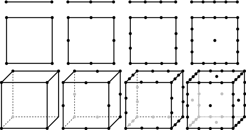
Fig. 1. Degrees of freedom for ${\mathcal{S}}_{r}(I^{n})$ for $r=1,2,3,4$, $n=1,2,3$. Dots indicate the number of degrees of freedom associated to each face.

Theorem 2.2 (Unisolvence).

The degrees of freedom specified in (2.2) are unisolvent for ${\mathcal{S}}_{r}(I^{n})$.

Proof.

First we note that number of degrees of freedom equals the dimension of the space. Indeed, there are $2^{n-d}\binom{n}{d}$ faces of the cube of dimension $d$ (obtained by fixing $n-d$ of the variables to $\pm 1$) and, for $f$ of dimension $d$, $\dim{\mathcal{P}}_{r-2d}(f)=\binom{r-d}{d}$, so the total number of degrees of freedom proposed is precisely $\dim{\mathcal{S}}_{r}(I^{n})$ given by (2.1). It remains to show that if $u\in{\mathcal{S}}_{r}(I^{n})$ and all the quantities in (2.2) vanish, then $u$ vanishes. We do this by induction on $n$, the case $n=1$ being trivial. Let $F$ be a face of $I^{n}$ of dimension $n-1$ and let $U=u|_{F}$. The $U$ is a polynomial in $n-1$ variables with superlinear degree at most $r$, i.e., $U\in{\mathcal{S}}_{r}(F)$. Moreover, if $f$ is any face of $F$ of dimension $d$, and $q\in{\mathcal{P}}_{r-2d}(f)$, then $\int_{f}Uq=\int_{f}uq=0$. Therefore, by the inductive hypothesis, $U$ vanishes. In this way, we see that $u$ vanishes on all its faces, i.e., whenever we fix some $x_{i}$ to $\pm 1$. Therefore

$$u=(1-x_{1}^{2})\cdots(1-x_{n}^{2})\,p$$

for some polynomial $p$. Note that $\deg_{2}u=2n+\deg p$. Therefore $\deg p\leq r-2n$, and we make take $f=I^{n}$ and $q=p$ in (2.2) to find

$$\int_{I^{n}}(1-x_{1}^{2})\cdots(1-x_{n}^{2})\,p^{2}=0.$$

It follows that $p=0$. ∎

In the proof of unisolvence we established that the degrees of freedom associated to a face and its subfaces determine the restriction of $u$ to the face. This is important, since it implies that an assembled serendipity finite element function is continuous.

3. Geometric decomposition

In this section we give a geometric decomposition of ${\mathcal{S}}_{r}(I^{n})$, by which we mean a direct sum decomposition into subspaces associated to the faces. Such a decomposition can be used to derive explicit local bases which are useful for the efficient implementation of the elements, and also for insight.

First we introduce some notation. Let $\Delta_{d}(I^{n})$ denote the set of faces of the $n$-cube of dimension $d$ and $\Delta(I^{n})=\bigcup_{d=0}^{n}\Delta_{d}(I^{n})$ the set of all faces of all dimensions. A face $f\in\Delta_{d}(I^{n})$ is determined by the equations $x_{j}=c_{j}$ for $j\in J$ where $J\subset\mathbb{N}_{n}$ is a set of cardinality $n-d$ and each $c_{j}\in\{-1,1\}$. We define the bubble function for $f$ as

$$b_{f}=\prod_{j\in J^{c}}(1-x_{j}^{2})\prod_{j\in J}(1+c_{j}x_{j}),$$

the unique (up to constant multiple) nontrivial polynomial of lowest degree vanishing on the $(n-1)$-dimensional faces of $I^{n}$ which do not contain $f$. Note that $b_{f}$ is strictly positive on the relative interior of $f$ and vanishes on all faces of $I^{n}$ which do not contain $f$. For $s\geq 0$ we denote by ${\mathcal{P}}_{s}^{f}(I^{n})$ the space of polynomials of degree at most $s$ in the $d$ variables $x_{j}$, $j\in J^{c}$. If $d=0$, then ${\mathcal{P}}_{s}^{f}(I^{n})$ is understood to be $\mathbb{R}$.

To a face $f$ of dimension $d$ we associate the space of polynomials $V_{f}:={\mathcal{P}}_{r-2d}^{f}(I^{n})b_{f}$. By definition, any element $q\in V_{f}$ has the form $q=p\prod_{j\in J}(x_{j}+c_{j})$ where $p\in{\mathcal{P}}_{r}^{f}(I^{n})$, and so $\deg_{2}q\leq r$. Thus $V_{f}\subset{\mathcal{S}}_{r}(I^{n})$. The following theorem states that they do indeed form a geometric decomposition.

Theorem 3.1 (Geometric decomposition of the serendipity space).

Let ${\mathcal{S}}_{r}(I^{n})$ denote the serendipity space of degree $r$, and for each $f\in\Delta_{d}(I^{n})$, let $V_{f}={\mathcal{P}}_{r-2d}^{f}(I^{n})b_{f}$. Then

(3.1) $${\mathcal{S}}_{r}(I^{n})=\sum_{f\in\Delta(I^{n})}V_{f}.$$

Moreover, the sum is direct.

Proof.

Clearly $\dim V_{f}=\dim P_{r-2d}^{f}(I^{n})=\binom{r-d}{d}$, and so (2.1) implies that

$$\dim{\mathcal{S}}_{r}(I^{n})=\sum_{f\in\Delta(I^{n})}\dim V_{f}.$$

Hence, it is sufficient to prove that if $p$ is a monomial with superlinear degree $\leq r$, then $p\in\sum_{f}V_{f}$. Write $p=x_{1}^{\alpha_{1}}\cdots x_{n}^{\alpha_{n}}$ and let

$$J_{0}=\{\,i\in\mathbb{N}_{n}\,|\,\alpha_{i}=0\,\},\quad J_{1}=\{\,i\in\mathbb{N}_{n}\,|\,\alpha_{i}=1\,\},\quad J_{2}=(J_{0}\cup J_{1})^{c},$$

denote the sets indexing the variables in which $p$ is constant, linear, and superlinear, respectively. By assumption, $\sum_{j\in J_{2}}\alpha_{j}\leq r$. Now we expand

$$x_{j}^{\alpha_{j}}=\begin{cases}\frac{1}{2}(1+x_{j})+\frac{1}{2}(1-x_{j}),&j\in J_{0},\\ \frac{1}{2}(1+x_{j})-\frac{1}{2}(1-x_{j}),&j\in J_{1},\\ \frac{1}{2}(1+x_{j})+\frac{(-1)^{\alpha_{j}}}{2}(1-x_{j})+(1-x_{j}^{2})r_{j}(x_{j}),&j\in J_{2},\end{cases}$$

where $\deg r_{j}=\alpha_{j}-2$, and insert these into $p=x_{1}^{\alpha_{1}}\cdots x_{n}^{\alpha_{n}}$. We find that $p$ is a linear combination of terms of the form

(3.2) $$q=\prod_{j\in J^{\prime}}r_{j}(x_{j})(1-x_{j}^{2})\prod_{j\in J^{\prime\prime}\cup J_{0}\cup J_{1}}(1\pm x_{j}),$$

where $J^{\prime}$ and $J^{\prime\prime}$ partition $J_{2}$. Let $f$ be the face given by $1\mp x_{j}=0$, $j\in J^{\prime\prime}\cup J_{0}\cup J_{1}$, where the signs are chosen opposite to those on (3.2). Then $\dim f=\#J^{\prime}$ and $q=rb_{f}$ with $r\in{\mathcal{P}}_{s}^{f}(I^{n})$, $s=\sum_{j\in J^{\prime}}(\alpha_{j}-2)\leq r-2\dim f$. This shows that $q\in V_{f}$ and $p\in\sum_{f}V_{f}$, as desired. ∎

References

- [1] Thomas J. R. Hughes, The finite element method, Prentice Hall Inc., Englewood Cliffs, NJ, 1987, Linear static and dynamic finite element analysis, With the collaboration of Robert M. Ferencz and Arthur M. Raefsky.
- [2] Victor N. Kaliakin, Introduction to approximate solution techniques, numerical modeling, & finite element methods, CRC, 2001, Civil and Environmental Engineering.
- [3] Jan Mandel, Iterative solvers by substructuring for the -version finite element method, Comput. Methods Appl. Mech. Engrg. 80 (1990), no. 1-3, 117–128, Spectral and high order methods for partial differential equations (Como, 1989).
- [4] Gilbert Strang and George J. Fix, An analysis of the finite element method, Prentice-Hall Inc., Englewood Cliffs, N. J., 1973, Prentice-Hall Series in Automatic Computation.
- [5] Barna Szabó and Ivo Babuška, Finite element analysis, A Wiley-Interscience Publication, John Wiley & Sons Inc., New York, 1991.
- [6] O. C. Zinkiewicz, R. L. Taylor, and J. Z. Zhu, The finite element method: its basis and fundamentals, vol. 1, sixth ed., Butterworth-Heinemann, 2005.