Schwarzschild black holes as unipolar inductors: expected electromagnetic power of a merger

Abstract

The motion of a Schwarzschild black hole with velocity $v_{0}=\beta_{0}c$ through a constant magnetic field  $B_{0}$ in vacuum induces a component of the electric field  along the magnetic field, generating a non-zero second Poincare electromagnetic invariant ${}^{*}F\cdot F\neq 0$. This will produce (e.g., via radiative effects and vacuum breakdown) an electric charge density of the order of $\rho_{\rm ind}=B_{0}\beta_{0}/(2\pi eR_{G})$, where $R_{G}=2GM/c^{2}$ is the Schwarzschild radius and $M$ is the mass of the black hole; the charge density $\rho_{\rm ind}$ is similar to the Goldreich-Julian density.

The magnetospheres of moving black holes resemble in many respects the magnetospheres of rotationally-powered pulsars, with pair formation fronts and outer gaps, where the sign of the induced charge changes. As a result, the black hole will generate bipolar electromagnetic jets each consisting of two counter-aligned current flows (four current flows total), each carrying an electric current of the order $I\approx eB_{0}R_{G}\beta_{0}$. The electromagnetic power of the jets is $L\approx(GM)^{2}B_{0}^{2}\beta_{0}^{2}/c^{3}$; for a particular case of merging black holes the resulting Poynting power is $L\approx{(GM)^{3}B_{0}^{2}/(c^{5}R)}$, where $R$ is the radius of the orbit.

In addition, in limited regions near the horizon the first electromagnetic invariant changes sign, so that the induced electric field becomes larger than the magnetic field, $E>B$. As a result, there will be local dissipation of the magnetic field close to the horizon, within a region with the radial extent $\Delta R\approx R_{G}\beta_{0}$.

The total energy loss from a system of merging black holes is a sum of two components with similar powers, one due to the rotation of space-time within the orbit, driven by the non-zero angular momentum in the system, and the other due to the linear motion of the black holes through the magnetic field.

Since the resulting electrodynamics is in many respects similar to pulsars, merging black holes may generate coherent radio and high energy emission beamed approximately along the orbital normal. In addition, merging black holes may produce observable wind-driven cavities.

PACS numbers: 04.30.Tv, 95.85.Sz

I Introduction

Observations of an electromagnetic signal accompanying black hole merger is most desirable, as it will provide crucial information on the location and the physical properties of the event. Two types of electromagnetic  signal can be expected from merging black holes. First, merging black holes induce perturbations in the surrounding gas Armitage and Natarajan (2002); Krolik (2010); Milosavljević and Phinney (2005); van Meter et al. (2010). The resulting electromagnetic signal is then subject to great uncertainty and naturally depends on the complicated non-linear fluid behavior of the system. One of the problems is that at late stages of the merger there should be little gas inside the orbit since the timescale for shrinkage of the binary orbit by gravitational wave radiation becomes shorter than the timescale for mass inflow due to viscose stresses in the disk Milosavljević and Phinney (2005). It is then hard to excite transient dissipative processes in a faraway accretion disk.

Alternatively, external gas can support electric currents that create large scales magnetic fields. Motion of black holes in this externally supplied magnetic field can then lead to electromagnetic extraction of energy. Qualitatively, there are two distinct possibilities for the electromagnetic extraction of energy from spiraling black holes. First, the system of two orbiting black holes possesses non-zero angular momentum, which induces rotation of space time. Rotating space-time can generate electromagnetic outflows, in a manner similar to the classical Faraday disk. This is the physics behind the Blandford & Znajek Blandford and Znajek (1977) process of extracting the rotational power of a black hole. Below we refer to this mechanism as the Faraday disk mechanism. This mechanism has been previously considered in Ref. Lyutikov (2010). For a given magnetic field, the resulting power can be estimated using the Faraday disk scaling, $L_{EM,F}\sim R^{2}B_{0}^{2}c(\Omega R/c)^{2}$, where $R$ is the orbital radius and $\Omega$ is the typical angular velocity of the rotation of the space-time within the black holes’ orbit, $\Omega\sim{(GM)^{3/2}/(c^{2}R^{5/2}})$. The resulting Poynting flux is then

$$L_{EM,F}\approx{G^{3}M^{3}\over c^{5}R}B_{0}^{2}$$ (1)

In a separate, physically distinct process, which we consider in this paper, the linear motion of a Schwarzschild black hole will generate the electric potential drop across the black hole, so that a black hole will effectively operate as a unipolar inductor, in a way somewhat similar to the planet Io moving in Jupiter’s magnetic field  Goldreich and Lynden-Bell (1969). Classically, the motion of a conductor though the magnetic field generates in the frame of a conductor an electric field ${\bf E}=-{\bf v}\times{\bf B}$. This induced electric field will generally have a normal component to the surface of the conductor. As a result, surface charges will be generated; they will produce their own electric field, now with a component parallel to the initial magnetic field. This electric field drives currents along magnetic field lines; dissipation of these currents is responsible for non-thermal radio through X-ray emission of the Jupiter magnetosphere. An important difference of the unipolar induction mechanism considered in the present paper from the classical unipolar inductor is that in the case of a black hole no physical charges are needed to produce $E_{\parallel}$. Parallel electric field appears in complete vacuum due to the curvature of space.

A qualitative estimate of the resulting Poynting power may be obtained from the following reasoning. For a conductor of length $l$ moving with velocity $v_{0}=\beta_{0}c$ through magnetic field $B_{0}$ the resulting potential difference $\Delta\Phi\sim\beta_{0}LB$. If the resulting outflow is relativistic, the electromagnetic power can be estimated as $L_{EM}\sim\Delta\Phi^{2}c=\beta_{0}^{2}B_{0}^{2}l^{2}c$ (see also McWilliams (2010)). In the case of orbiting black hole, estimating $l\sim R_{G}$ (the Schwarzschild radius) and $\beta_{0}=\sqrt{R_{G}/R}$, the expected power of unipolar inductor turns out to be the same as that of the Faraday disk mechanism, Eq. (1).

Thus, the estimates of the electromagnetic powers due to rotation of the space-time and due to linear motion of a black hole with Keplerian velocity turn out to be similar, given by Eq. (1); we view this as a coincidence. Though in both cases the power eventually comes from the inductive electric field, the underlying physics is different in the two case. One mechanism requires non-zero angular momentum, while the other does not. A total energy loss from a system of merging black holes is a sum of two components with similar powers, one due to the rotation of space-time within the orbit, another due to linear motion of the black holes through magnetic field.

Previously, in Refs. Palenzuela et al. (2010a, b); Neilsen et al. (2010) a number of force-free simulations of black hole magnetospheres were performed. In the case of the orbiting black holes the authors mostly studied the electromagnetic power due to linear motion of black hole, and not due to rotation of the space-time within the orbit. The present paper offers explanations and parameter scalings of these numerical simulation.

II Static electromagnetic fields in Schwarzschild metric

Consider vacuum stationary homogeneous electromagnetic fields in Schwarzschild metric. Though the structure of a constant electromagnetic fields in Schwarzschild  metric is well known (Wald, 1974; Hanni and Ruffini, 1976; Ernst, 1976; Beskin, 1997), here we briefly re-derive it here for completeness. Adopting a Schwarzschild metric

$$ds^{2}=-\alpha^{2}dt^{2}+{1\over\alpha^{2}}dr^{2}+r^{2}\left(d\theta^{2}+\sin^{2}\theta d\phi^{2}\right)$$ (2)

where $\alpha=\sqrt{1-2M/r}$, the relevant vacuum Maxwell equations

$$\partial_{\nu}\left(\sqrt{-g}F^{\mu\nu}\right)=0,$$ (3)

($F_{\mu\nu}=A_{[\mu,\nu]}$ is Maxwell tensor) for the non-vanishing components of the vector potential $A_{0}(r,\theta^{\prime})$ and $A_{\phi}(r,\theta)$ (here $\theta^{\prime}$ and $\theta$ are angles with respect to the axes aligned with the electric and magnetic field at infinity) give

$$\alpha^{2}\partial_{r}(r^{2}\partial_{r}A_{0})+{1\over\sin\theta^{\prime}}\partial_{\theta^{\prime}}(\sin\theta^{\prime}\partial_{\theta^{\prime}}A_{0})=0\mbox{}$$

$$r^{2}\partial_{r}\alpha^{2}\partial_{r}A_{\phi}+\sin\theta\partial_{\theta}\left({1\over\sin\theta}\partial_{\theta}A_{\phi}\right)=0.$$ (4)

(In vacuum, the same relations hold for the dual Maxwell tensor ${}^{*}F_{\mu\nu}$; in that case the equations for $A_{0}$ and $A_{\phi}$ switch.) The potentials corresponding to constant fields at infinity are

$$A_{0}=E_{0}(r-2M)\cos\theta^{\prime}\mbox{}$$

$$A_{\phi}={B_{0}\over 2}r^{2}\sin^{2}\theta$$ (5)

The electromagnetic fields

$${\bf E}=(1/\alpha)\nabla A_{0}=E_{0}\left({\cos\theta^{\prime}}{\bf e}_{r}-\alpha\sin\theta^{\prime}{\bf e}_{\theta}\right)\mbox{}$$

$${\bf B}={\nabla\times A_{\phi}{\bf e}_{\phi}}=B_{0}\left({\cos\theta}{\bf e}_{r}-\alpha\sin\theta{\bf e}_{\theta}\right)$$ (6)

where $\nabla$ is a covariant derivative, with a corresponding unit radial vector ${\bf\hat{e}}_{r}=\alpha\partial_{r}$. The structure of the electric and magnetic fields is the same, as follows from the duality transformation in vacuum.

The above relations can be obtained in a more conventional way by using the alternative $3+1$ formulation of the General Relativity Thorne et al. (1986), in which case the Maxwell equations in the more general Kerr metric take the form

$$\nabla\cdot{\bf E}=4\pi\rho\mbox{}$$

$$\nabla\cdot{\bf B}=0\mbox{}$$

$$\nabla\times(\alpha{\bf B})=4\pi\alpha{\bf j}+D_{t}{\bf E}\mbox{}$$

$$\nabla\times(\alpha{\bf E})=-D_{t}{\bf B}$$ (7)

where $D_{t}=\partial_{t}-{\cal L}_{\vec{\beta}}$ is the total time derivative, including Lie derivative along the velocity of the zero angular momentum observers (ZAMOs). For Schwarzschild metric $\vec{\beta}=0$ and in the stationary case $D_{t}\equiv 0$. Electromagnetic fields in Eq. (7) are those measured by a stationary local observer in terms of local time. The fields $\alpha{\bf E}$ and $\alpha{\bf B}$ are those measured by a local observer in terms of Schwarzschild time $t$.

Since we expect that the non-zero charge will eventually be created, we give here the complete Laplace equation for the electric potential $A_{0}$ in presence of non-zero charge density

$$\nabla{1\over\alpha}\nabla A_{0}=4\pi\rho\mbox{}$$

$${1\over r^{2}}\partial_{r}(r^{2}\partial_{r}A_{0})+{1\over\alpha^{2}r\sin\theta^{\prime}}\partial_{\theta}(\sin\theta\partial_{\theta}A_{0})+{1\over\alpha^{2}r^{2}\sin^{2}\theta}\partial_{\phi}^{2}A_{0}=4\pi{\rho\over\alpha}$$ (8)

cf. (Linet, 1976, Eq. 10).

The shape of the field lines (6) is given by

$$\sin\theta=2e^{-2(1-\alpha)}{1-\alpha\over 1+\alpha}{r_{\perp,0}\over M}$$ (9)

where $r_{\perp,0}$ is the radial cylindrical distance from the axis of a given field line at infinity. The last field line that intersects the black hole at $\theta=\pi/2$ has initial $r_{\perp,0}=e^{2}M/2$ and is given by $\sin\theta=2{e^{2\alpha}\over(1+\alpha)}{M\over r}$. Note, that though the surfaces of constant magnetic flux are cylinders $r\sin\theta={\rm constant}$ (corresponding to $A_{\phi}=$ constant), on the horizon the magnetic field  in Schwarzschild coordinates becomes radial. This is naturally impossible at the point $r=2M,\theta=\pi/2$, but at that point the magnetic field  is zero. This seeming inconsistency can be resolved in terms of embedding diagrams Hanni and Ruffini (1976).

By construction fields (6) correspond to $\nabla\cdot{\bf E}=0$, so any local observer would measures zero charge density. On the other hand, judging by the shape of electric field lines in coordinates $r-\theta$, the observer at infinity will infer a dipolar-like charge distribution

$$\rho_{eff}=\nabla_{\rm nc}\cdot{\bf E}=2\left(1-\alpha\right){\cos\theta^{\prime}\over r}E_{0}$$ (10)

Here $\nabla_{\rm nc}$ denotes the non-covariant differentiation with respect to coordinates $r-\theta$. The effective charge is concentrated near the black hole  so at large distances the black hole effectively has a surface charge

$$\sigma_{eff}={1\over 4\pi}\int_{2M}^{\infty}\rho_{eff}dr={\ln(e/2)\over\pi}E_{0}\cos\theta^{\prime}$$ (11)

We stress that there are no physical charges present: the shape of electric field lines in the chosen metric is modified by gravity, not electric charges. Also, the shape of field lines and the value of the effective surface density depends on the choice of coordinates and a given set of observers.

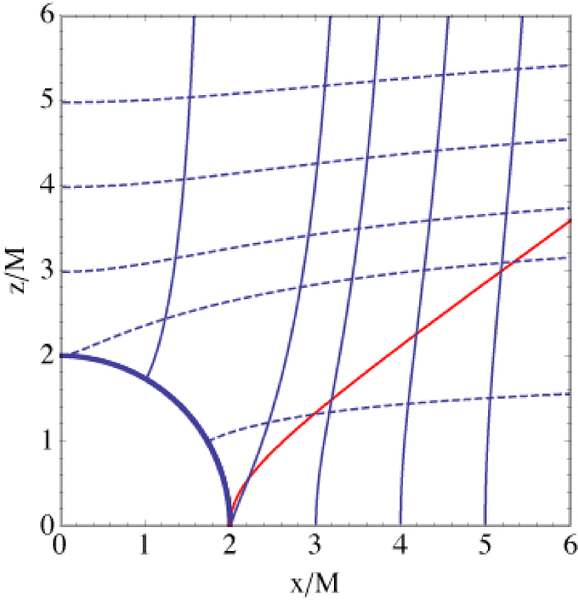
Figure 1: Shape of magnetic (solid lines aligning with $z$ axis) and electric (dashed lines, aligning with $x$ axis) field lines in the $x-z$ plane for vacuum Schwarzschild black hole. Red curve (in the online color image) starting at the point $\theta=\pi/2$, $r=2M$ is the shape of the outer gap, where the sign of the induced charges changes.

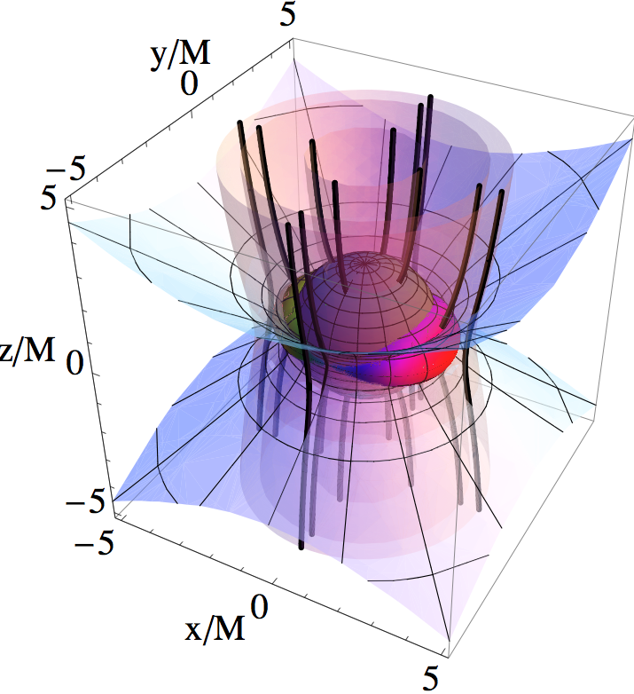
Figure 2: 3D view of the black hole magnetosphere. Magnetic field (thick solid lines together with magnetic surfaces) is along $z$ axis at large distance, the black hole is moving along the $y$ direction. The central sphere of radius $r=2M$ is the Schwarzschild radius. Two limited regions near the equatorial plane approximately aligned with the $x$ axis are bounded by the surfaces $E=B$. On the nearly conical surfaces originating at the magnetic equator the induced charge density is zero. This particular plot is for $\beta_{0}=1/2$.

III black hole in electromagnetic fields orthogonal at infinity.

Let us next assume that in a particular reference frame at large distances from the black hole the magnetic field is along $-{\bf e}_{z}$ direction, while in this reference frame the electric field is zero. A black hole is moving orthogonally to magnetic field with velocity $\beta_{0}=v_{0}/c$ along $y$ direction. In the frame of the black hole, at large distances $r\gg M$, there is then a static electric field ${\bf E}_{0}=-{\bf v}\times{\bf B}_{0}=\beta_{0}B_{0}{\bf e}_{x}$, $E_{0}=\beta_{0}B_{0}$. (In this section we define $B_{0}$ as the value of magnetic field in the frame where black hole is at rest; it is related to the value in the frame where electric field is vanishing by a simple Lorentz transformation). Thus, in the frame of the hole the electric and magnetic fields are given by Eq. (6), where $\theta^{\prime}$ is a polar angle with respect to the $x$ axis, $\cos\theta^{\prime}=\sin\theta\cos\phi$. The electromagnetic invariants are

$$B^{2}-E^{2}=B_{0}^{2}(1-\beta_{0}^{2})+2\left(\beta_{0}^{2}(\cos^{2}\theta\cos^{2}\phi+\sin^{2}\phi)-\sin^{2}\theta\right){B_{0}^{2}M\over r}\mbox{}$$

$${\bf E}\cdot{\bf B}\equiv-{{\rm Det}|F_{\mu\nu}|\over\sqrt{-g}}=-\cos\phi\sin 2\theta\beta_{0}B_{0}^{2}{M\over r}$$ (12)

while the parallel electric field is

$$E_{\parallel}=-\cos\phi\sin 2\theta{M\over r\sqrt{1-2\sin^{2}\theta M/r}}E_{0}$$ (13)

Eqns. (12) highlight two important points. The second Poincare electromagnetic invariants is generally non-zero, ${\bf E}\cdot{\bf B}\not\equiv 0$. The first Poincare invariant changes sign on the surface

$$r={2M\left(\sin^{2}\theta-\beta_{0}^{2}(\cos^{2}\theta\cos^{2}\phi-\sin^{2}\phi)\right)\over 1-\beta_{0}^{2}}$$ (14)

This occurs close to the horizon around points $\{\theta\approx\pi/2,\phi\approx 0,\pi\}$ within a region ${\Delta r\over 2M}\approx\beta_{0}^{2}/(1-\beta_{0}^{2})$, see Fig. 2.

We expect that in astrophysical environment $E_{\parallel}$ will be decreased by pair creation (see §IV). Still, the perpendicular component of the electric field  $E_{\perp}$ becomes larger than the magnetic field at points

$$\left(1-{2M\sin^{2}\theta\over r}\right)^{2}=\beta_{0}^{2}\alpha\left(1-{2M\sin^{2}\theta\sin^{2}\phi\over r}\right)$$ (15)

The region bounded by this surface has a shape similar to the one where $E=B$, Eq. (14), see Fig. 3.

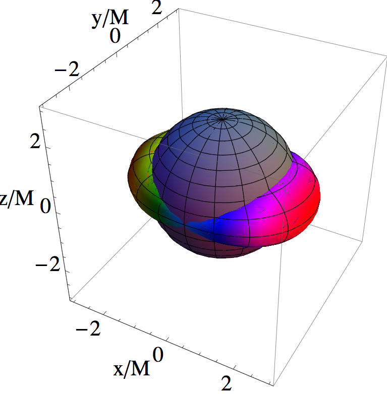
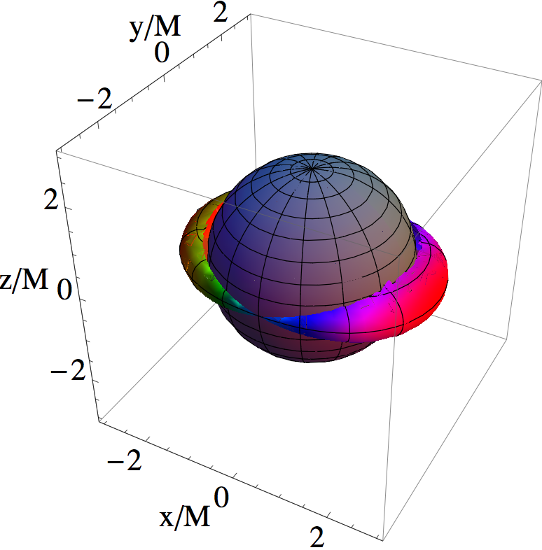
Figure 3: 3D view of the surfaces bounding the regions where $E>B$ (Left Panel) and $E_{\perp}>B$ (Right Panel) for $\beta_{0}=0.5$. The central sphere of radius $r=2M$ is the Schwarzschild radius. False colors (in the online version) in this figure and Figs. 4 and 9 are chosen for presentation purpose only.

Since we expect that a plasma will be generated due to vacuum breakdown, we can define the plasma drift velocity (assuming $\beta_{d}<1$, see below)

$${\vec{\beta_{d}}}={\bf E}\times{\bf B}/B^{2}={\alpha\over 1-2M\sin^{2}\theta/r}\left({\alpha}\sin\theta\sin\phi{\bf e}_{r}+\cos\theta\sin\phi{\bf e}_{\theta}+\cos\phi{\bf e}_{\phi}\right)\beta_{0}$$ (16)

It is directed along $y$ axis at large distances, but becomes complicated near the hole. Most importantly, the value of $v$ is not bound. Close to the points $\theta=\pi/2,\phi=0,\pi$, the velocity diverges as $\beta_{d}\approx\beta_{0}/\alpha$. This is related to the previously mentioned fact that the second electromagnetic invariant changes sign close to these points.

IV Magnetospheres of moving Schwarzschild black holes

IV.1 Induced charge density

In the previous section we showed that the motion of a Schwarzschild black hole through magnetic field in vacuum generates non-zero second Poincare electromagnetic invariant (parallel electric field) and regions where the first Poincare changes sign, $E>B$. In vacuum this would have been the end of the story, so to say. In reality, astrophysical plasmas tolerate neither large parallel electric field, nor regions of $E>B$: any stray particle will be accelerated by electric field and will produce an electron-positron pair via various radiative effects. The resulting pair plasma will try to screen the initial parallel electric field, by producing a charge density required to have ${\bf E}_{\parallel}=0$.

Thus, we expect that around astrophysical black holes moving in external magnetic field  a non-zero charge density will appear, that satisfies the equation (8) with induced electric field

$${\bf E}_{\rm ind}=E_{\parallel}\hat{\bf b}$$ (17)

where

$$\hat{\bf b}={1\over\sqrt{1-(2M/r)\sin^{2}\theta}}\left(-{\cos\theta}{\bf e}_{r}+\alpha\sin\theta{\bf e}_{\theta}\right)$$ (18)

is a unit vector along magnetic field. The corresponding charge density, see Fig. 4

$$\rho_{\rm ind}={1\over 4\pi}\nabla\cdot{\bf E}={\alpha\over\pi}{\left(1+\left(M/r-3/2\right)\sin^{2}\theta\right)\over(1-(2M/r)\sin^{2}\theta)^{2}}\cos\phi\sin\theta{ME_{0}\over r^{2}}$$ (19)

The typical value of charge density $\rho_{0}$ is

$$\rho_{0}={\beta_{0}B_{0}\over 4\pi M}={B_{0}(v_{0}/R_{G})\over 2\pi c}$$ (20)

This reminds the Goldreich-Julian charge density (Goldreich and Julian, 1969) if we substitute $v_{0}/R_{G}\rightarrow\Omega_{eff}$.

At large distance from the black hole  the charge density is

$$\rho_{\rm ind}\approx{(1+3\cos 2\theta)\cos\phi\sin\theta M^{2}\over r^{2}}\rho_{0}$$ (21)

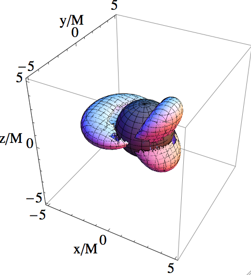
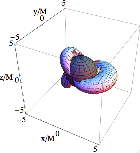
Figure 4: Surfaces of constant charge density $\rho_{\rm ind}=+|{\rm Const}|$ (Left Panel) and $\rho_{\rm ind}=-|{\rm Const}|$ (Right Panel) for ${\rm Const}=2\times 10^{-2}\rho_{0}$ and $\beta_{0}=0.5$.

On the magnetic equator $\theta=\pi/2$ the charge density is

$$\rho_{ind,\theta=\pi/2}=2{\rho_{0}\over\alpha}{M^{2}\over r^{2}}\cos\phi$$ (22)

It diverges on the horizon. The charge density close to the horizon $\rho_{ind,h}$ is

$$\rho_{ind}={\alpha\rho_{0}}{\cos\phi\sin\theta\over\cos^{2}\theta}$$ (23)

It diverges near the equator.

The point $r=2M$, $\theta=\pi/2$ is a special one, as can be seen from the fact that the limit of Eq. (23) for $\theta\rightarrow\pi/2$ does not coincide with the limit $r\rightarrow 2M$ of Eq. (22). This can be traced to the fact that on the one hand, the lines of force must cross horizon orthogonally (e.g.,  Hanni and Ruffini, 1976), yet on the other hand they must lay on cylinders $r\sin\theta={\rm constant}$ (see Eq. (6)). These two conditions are inconsistent at the point $\theta=\pi/2$, $r\rightarrow 2M$. Recall also that the magnetic field is zero at this point, Eq. (6), while experiencing a kink, clearly seen in the embedding diagram (Hanni and Ruffini, 1976).

IV.2 Plasma response

Similarly to the case of rotating neutron stars, two alternative possibilities exist with respect to the dynamical response of the system to the required charge density. First, the overall plasma distribution can provide a static distribution of the required charge density and the system will overall be quiet, without strong electromagnetic outflows. In case of pulsars, this approach is advocated in Ref. Michel (1979). This scenario is supported by the fact that direct PIC simulations of the pulsar magnetospheres so far failed to produced an outflow: the system indeed just relaxes to a nearly steady-state configuration Smith et al. (2001). It is expected that secular instabilities of the resulting charged configurations (e.g., diocotron instability, Pétri et al., 2002) may eventually lead to the formation of the jets (Spitkovsky, priv. comm.).

Alternatively (and this viewpoint is supported by majority of pulsar theorists), static charge configuration cannot be established on magnetic field lines connecting to infinity, resulting in the formation of the wind Goldreich and Julian (1969). Fluid simulation of pulsar magnetospheres support this paradigm Spitkovsky (2006). Since in our case all magnetic field lines are connected to infinity, large parallel electric fields  will lead to plasma outflow, which would qualitatively resemble plasma outflow on the open lines of pulsar magnetospheres.

We accept the paradigm that in the case of black holes, similar to the pulsar magnetospheres, parallel electric fields will lead to vacuum breakdown, generation of primary beam and a dense secondary plasma. In this Section we investigate the resulting electromagnetic structure of the black hole magnetospheres.

IV.3 Pair formation front

A black hole  moving with velocity $v_{0}=\beta_{0}c$ through magnetic field $B_{0}$ creates a potential drop of the order $\Delta\Phi\approx\beta_{0}r_{G}B_{0}$. For example, for a black hole of mass $M=10^{6}M_{\odot}m_{6}$ moving on the orbit $\xi\gg 1$ times larger than the Schwarzschild radius, $R_{\rm orb}=\xi r_{G}$, in a given magnetic field, the resulting potential is $\Phi\approx 5\times 10^{13}\,{\rm V}\left({B\over 1{\rm G}}\right)m_{6}\xi^{-1/2}$. This will result in a particle energy, which is typically much larger than the one required to break the vacuum. For example, in pulsar magnetospheres, the pulsar death line corresponds approximately to $\Phi\approx 10^{9}$ V (e.g.,  Arons and Scharlemann, 1979; Hibschman and Arons, 2001). Though radiative processes and the photon fields around pulsars and around black holes can be substantially different, in case of black holes the available potential is many order of magnitude larger than the one corresponding to the pulsar death line. This should ensure the vacuum breakdown and the formation of the secondary pair plasma in black hole magnetospheres.

For a given parallel electric field, Eq. (12) and a given shape of field lines, Eq. (9), we can calculated the total potential drop along a field line $\Delta\Phi=\int E_{\parallel}ds$, where $ds$ is taken along a given field line. For magnetic field lines that intersect the black hole horizon (those that have $r_{\perp,0}<e^{2}M/2$) the lower limit of integration is on the horizon, while for those field lines than miss the hole the lower limit of integration is at magnetic equator. After a particle gains sufficient energy $e\Delta\Phi_{\rm crit}$ to break the vacuum via radiative effects, a dense flow of the secondary particles will screen the resulting parallel electric field. We can calculate the shape of this so called pair formation front (equipotential surface) by requiring $\int E_{\parallel}ds=e\Delta\Phi_{\rm crit}$, see Fig. (5).

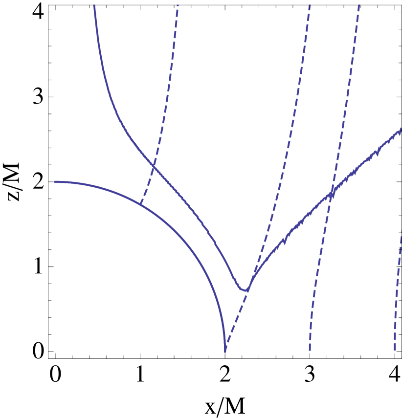
Figure 5: Structure of the equipotential surface in the $x-z$ plane (solid line). It is calculated by requiring that the potential drop along a given field lines equals some fiducial potential $\int E_{\parallel}ds=e\Delta\Phi_{\rm crit}$. Dashed lines are magnetic field lines.

Near the central field line the pair formation front is located at large distances from the black hole  since close the axis the electric field  is small, $E_{\parallel}\approx 2E_{0}\cos\phi{Mr_{\perp}\over r^{2}}$, where $r_{\perp}$ is the distance from the axis. To find the shape of a pair formation at large cylindrical distances, we note that magnetic field are nearly straight, while the parallel electric field bcomes $E_{\parallel}\approx\sin 2\theta\cos\phi(ME_{0}/r)$. A fixed potential drop is then achieved on surfaces satisfying

$$\sin\theta_{PPF}={e\Delta\Phi_{\rm crit}\over 2ME_{0}\cos\phi}.$$ (24)

Formally, the pari formation front extends to infinity.

IV.4 Large scale jets: quadruple current flow

Accepting the paradigm that the plasma will be streaming along magnetic field lines nearly with the speed of light, the charge density (19) will generate a current flow in the black hole magnetosphere. At large distances the sign of parallel electric field  and of the charge density depends on the quantity $\sin\theta\cos\phi$, Eqns. (12,19). Thus, two counter-aligned currents propagating along $z$ axis will be generated (four total separate current), separated the $y-z$ plane, Fig. 6.

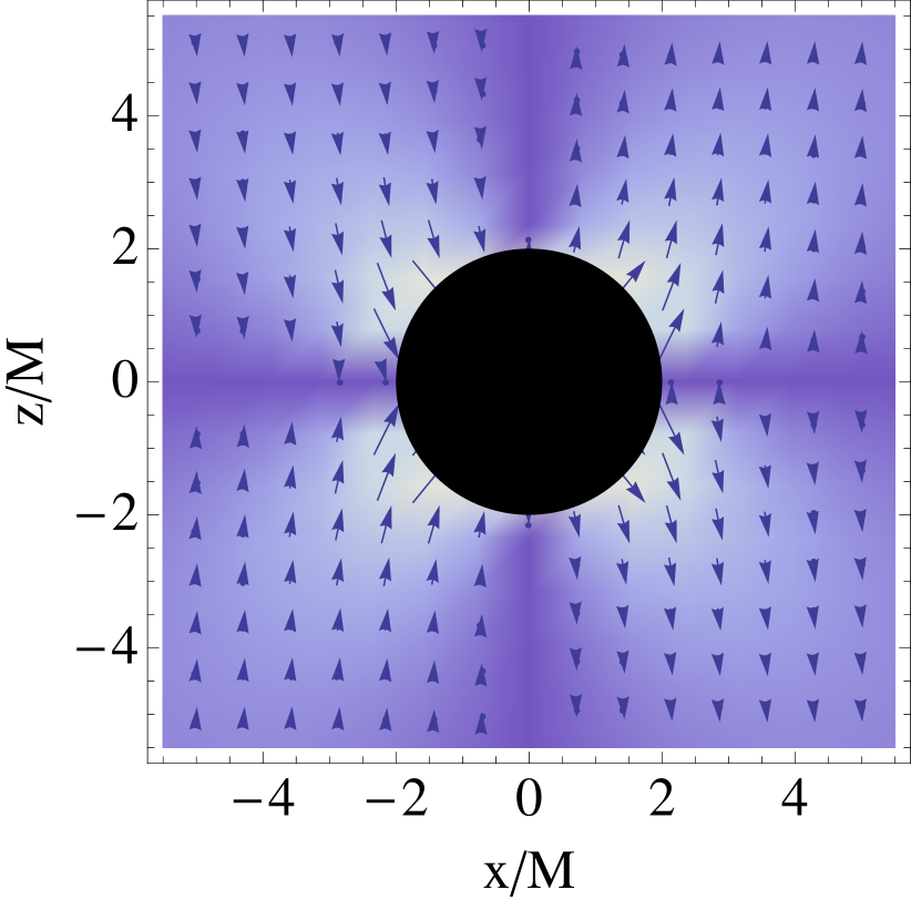
Figure 6: Value and direction of parallel electric field $E_{\parallel}$ in the plane $y=0$. Shadowing intensity is proportional to the absolute value of the electric field. The electric field has opposite direction in the four quadrants; as a result two counter-aligned current flows in each $\pm z$ direction will be generated.

Each quadrant of space carries a total current

$$I\approx r^{2}\int_{-\pi/2}^{\pi/2}d\phi\int_{0}^{\pi/2}\sin\theta d\theta\rho={\pi\over 4}M^{2}\rho_{0}={GM\beta_{0}B_{0}\over 16}$$ (25)

This current will produce toroidal magnetic field (for cylindrical radii $M\ll r_{\perp}\ll z$)

$$B_{\phi}\approx\beta_{0}{Mr_{\perp}^{2}\over 3\pi z^{3}}\cos\phi B_{0}\ll B_{0}$$ (26)

At a given cross-section $z=constant$, the toroidal magnetic field will roughly correspond to two equal counter-aligned current flows.

The regions of space with two counter-aligned currents propagating along $\pm z$ direction (corresponding to semi-spaces $x>0$ and $x<0$) will interact with each other. Since the currents are due to charge-separated flow, the interaction is both electric and magnetic. Oppositely charged currents have charge density per unit length $\lambda\approx M^{2}\rho_{0}$. The total electric force per unit length will be $F_{e}\approx\lambda^{2}/r=M^{4}\rho_{0}^{2}/r$. This electrostatic force will be nearly balanced (but not completely) by the magneto-static repulsive force of two counter-aligned currents $I$, Eq. (25). (The repulsive Lorentz force in this case will be smaller than the attractive Coulomb force by $1-v_{b}/c\ll 1$, where $v_{b}$ is the velocity of the particles from the primary beam.)

IV.5 Outer gaps

On some field lines the charge density changes along a field line, Fig. 7. By analogy with pulsar magnetospheres we will call the surfaces $\rho_{\rm ind}=0$ the “outer gaps”. The condition $\rho_{\rm ind}=0$ is satisfied on surfaces given by

$$r_{og}={2M\sin^{2}\theta\over 3\sin^{2}\theta-2}$$ (27)

The outer gaps touch the horizon at the equator and extend within polar angles $\arcsin\sqrt{2/3}<\theta<\pi-\arcsin\sqrt{2/3}$. At large distances the outer gap becomes a conical surface with $\cos 2\theta=\pm 1/3$, see Fig. 2.

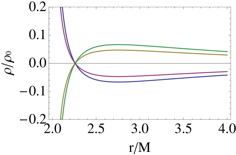
Figure 7: Charge density along magnetic field field lines starting at $\theta=\pi/2$ at different azimuthal angles $\phi=-(3/4)\pi,-\pi,0,\pi/2$ (top to bottom) at large $r$). The zero is at radii satisfying $\frac{4M^{2}e^{\frac{4\sqrt{r-2M}}{\sqrt{r}}}\left(\frac{M}{r}-\frac{3}{2}\right)}{\left(\sqrt{r-2M}+\sqrt{r}\right)^{4}}+1=0$, $r=2.260M$.

In addition, some magnetic field lines have the sign of the induced charge density changing two times along the field lines (this occurs along a narrow annular bunch of magnetic field lines that cross the horizon close to the magnetic equator).

V electromagnetic signals

V.1 Overall power

What electromagnetic signal can be expected from Schwarzschild black holes acting as a unipolar inductors? In a magnetically dominated medium with the effective impedance of free space, $\approx 4\pi/c$, the currents (25) will result in energy loss

$$L_{EM,u}\approx M^{2}E_{0}^{2}=M^{2}B_{0}^{2}\beta_{0}^{2}$$ (28)

The power (28) approximately equals $B_{\phi}^{2}r^{2}c$ with toroidal magnetic field given by the estimate (26). Equivalently, it arises due to initial electric field and the toroidal magnetic field (26) induced by the currents.

In particular, for a binary BH before merger, we can estimate the electric field as

$$E_{0}\sim B_{0}\sqrt{M/R}$$ (29)

where $R$ is the radius of the orbit. The resulting power is then

$$L_{EM,u}={M^{3}B_{0}^{2}\over R}\equiv{(GM)^{3}B_{0}^{2}\over c^{5}R}$$ (30)

where we reinstated the Newton’s constant and the speed of light. This is an estimate of the power lost by a black hole moving through constant magnetic field via unipolar inductor mechanism. It turns out to be of the same order as $L_{EM,F}$, Eq. (1), the power dissipated by the rotation of space with the black holes orbit via the Faraday disk mechanism Lyutikov (2010). Still, we stress that these powers comes from related but physically separate mechanisms: a Faradey-type electromagnetic outflow considered in Lyutikov (2010) and the linearly moving unipolar inductor discussed here (see also McWilliams (2010)). The power (30) is typically much smaller than the power carried away by gravitational waves at the later stages of the merger Lyutikov (2010).

V.2 Estimates of the magnetic field

The general expression for the Poynting power (30) depends on the strength of the magnetic field, which in case of merging astrophysical black holes  must be supported by the accretion disk and thus depend both on the microphysics of the disk dynamo Balbus and Hawley (1991) and the dynamical evolution of the binary black hole-accretion disk system Milosavljević and Phinney (2005); Krolik (2010).

Since the Poynting power (30) is the same as in the case of Faradey-type electromagnetic outflow driven by the rotation of space-time, we can use various estimates of magnetic field  and the merger dynamics discussed in Ref. Lyutikov (2010). Here we briefly restate the points.

Two stages of disk dynamics may be identified. At early times the loss of energy via gravitational radiation is slow enough, so that due to viscous diffusion the inner edge of the disk will be located close to the orbital radius, $R_{\rm d}\approx R$. At later times, for $R_{d}\leq\xi_{d}GM/c^{2},\,\xi_{d}\approx 40-100$ Milosavljević and Phinney (2005); O’Neill et al. (2009), the binary will decouple from the disk, undergoing a merger, while the inner edge of the disk remains fixed at $R_{d}$.

There are several estimates of magnetic field, which generally give similar values Lyutikov (2010). For example, magnetic field can be estimated assuming that a fraction $\eta_{E}$ of the Eddington luminosity is carried by magnetic field, $B^{2}\approx\eta_{E}L_{\rm Edd}/(cR_{d}^{2})$, (where $R_{d}\sim R$ before decoupling and $R\sim\xi_{d}R_{G}$ after decoupling)

$$B=\eta_{E}^{1/2}{(GM)^{1/2}\sqrt{m_{p}}\over\sqrt{\sigma_{T}}R_{d}}\approx 3\times 10^{4}\,{\rm G}\,m_{6}^{-1/2}\eta_{E,-1}^{1/2}\,\left({R_{d}\over R_{G}}\right)^{-1}$$ (31)

Thus, after decoupling magnetic field remains nearly constant within the orbit,

$$B_{d}\sim 300\,{\rm G}\,m_{6}^{-1/2}\eta_{E,-1}^{1/2}\,\xi_{d,2}^{-1}$$ (32)

The total power (30) in this case then becomes

$${L_{EM}\over L_{Edd}}=\eta_{E}{(GM)^{3}\over c^{6}RR_{d}^{2}}\leq\eta_{E}\,\xi_{d}^{-2}$$ (33)

The peak electromagnetic power is typically a fairly small fraction of the Eddington luminosity $L_{EM}\approx 10^{-5}-10^{-3}\,L_{Edd}$ and can realistically be observed at cosmological distances only for merger of very massive black holes, $M\geq 10^{8}M_{\odot}$.

Finally, comparing the power of the Schwarzschild black hole as unipolar inductor, Eq. (1) with the Blandford-Znajek power in a given magnetic field, $L_{BZ}\sim a^{2}B^{2}M^{2}$ ($a$ is the black hole spin parameter), gives

$${L_{EM}\over L_{BZ}}\approx{M\over a^{2}R}$$ (34)

Thus, for fast rotating black holes, $a\sim 1$, the power of the unipolar inductor is subdominant for $R\gg M$. (In addition, since during the merger the inner edge of the disk is at fairly large radii, $\geq 40-100R_{G}$, it is expected that the magnetic field on the black hole is smaller in the case of a merger).

V.3 Expected emission

Eqns (30-33) provide estimates of the total electromagnetic  power produced by a black hole in a form of a Poynting flux due to unipolar induction mechanism. A fraction of this power will be dissipated and converted into the observed radiation. Next, we discuss possible emission signatures. By analogy with pulsars, we expect several types of electromagnetic signal from black holes as unipolar inductors, approximately corresponding to magnetospheric and plerionic emission. In addition, in case of black holes we expect emission from regions with $E>B$.

V.3.1 Magnetospheric-type emission

As we discussed above, the magnetospheres of black holes  moving in magnetic field resemble in many respects the pulsar magnetospheres. Thus we may expect somewhat similar radiative signatures, though the details of the emission mechanisms proposed below must naturally be calculated independently for black hole  magnetospheres. Rotationally-powered pulsars produce, generally speaking, two types of radiation: coherent radio emission and high energy $X$-ray through $\gamma$-ray emission.

As we discussed in §IV.5, the sign of the induced charge density changes as a function of distance from the hole along a set of file lines, Figs. 2,7. One might expect that this will lead to effects qualitatively similar to the ones occurring in the so-called outer gaps in pulsar magnetospheres, where the sign of the Goldreich-Julian density changes Cheng et al. (1986). In particular, recent Fermi observations of pulsars show that high energy $\gamma$-ray emission is generated at the outer gaps Abdo et al. (2010). Similarly, we can expect that merging black holes will produce high energy emission, which will be preferentially beamed along the normal to the orbital plane. One might expect that, similar to pulsars, the emitted high energy power may reach tens of percent of the total electromagnetic power, Eq. (30).

The radiation physics of pulsar outer gaps is not well understood at the moment Hirotani et al. (2003). A particularly important difference between the pulsar and black hole magnetospheres considered here is that in case of pulsars the curvature radiation (in addition to inverse Compton processes) is an important ingredient. Magnetic fields in the magnetospheres of black holes will generally have drastically different - larger - radii of curvature, that would make curvature radiation unimportant (this cane be easily demonstrated following the estimates of the inverse curvature emission given below).

Another, in addition to curvature emission, important ingredient in the dynamics of the pulsar outer gaps is the inverse Compton (IC) emission. It will provide the dominant radiative friction effect to the particles accelerated in the black hole magnetospheres. Let us next estimate its properties. First, balancing the radiation friction force $\approx\gamma^{2}e^{4}U_{\rm ph}/(m_{e}^{2}c^{3})$, where $\gamma$ is the Lorentz factor of a particle and $U_{\rm ph}$ is the radiation field energy density, with the acceleration rate by the induced electric field, $eE_{0}c$, the terminal Lorentz factor becomes

$$\gamma={m_{e}c^{2}\sqrt{E_{0}\over e^{3}U_{\rm ph}}}$$ (35)

Estimating electric field as $E=\beta_{0}B_{0}=\sqrt{R_{G}/R_{\rm orb}}B_{0}$ and relating the radiation field energy density to Eddington luminosity, $U_{\rm ph}=L_{Edd}/(4\pi R_{\rm orb}^{2}c)$, we find

$$\gamma=\left({GMBm_{e}^{2}\sigma_{T}\over e^{3}m_{p}}\right)^{1/2}\xi^{3/4}=6\times 10^{6}\ ,B_{4}^{1/2}m_{6}^{1/2}\xi^{3/4}$$ (36)

where, we remind, $R_{\rm orb}=\xi r_{G}$.

We can then estimate the IC power produce by the leptons with typical density given by Eq. (20) within a typical volume $\approx R_{G}^{3}$,

$$L_{IC}\approx{\beta_{0}\over 2\pi\sqrt{\xi}}{B^{2}R_{G}^{2}c}=10^{40}\,{ergs^{-1}}B_{4}^{2}m_{6}^{2}\xi^{-1}$$ (37)

The typical frequency of IC emission is given by up-scattering of thermal photons of energy emitted at the inner edge of the accretions disk with energy

$$k_{B}T\approx\left({GM\dot{M}\over 8\pi\sigma_{SB}R^{3}}\right)^{1/4}$$ (38)

where $\sigma_{SB}$ is Stefan-Boltzmann constant, $k_{B}$ is Boltzmann constant and $\dot{M}$ is accretion rate. Scaling accretion rate $\dot{M}$ with Eddington luminosity, $\eta_{M}\dot{M}c^{2}=L_{Edd}$, where $\eta_{M}\sim 0.1$ is the accretion efficiency, we find

$$T=\left({m_{p}c^{5}\over 2\eta_{M}\sigma_{T}R^{3}}\right)^{1/4}\approx 120\,{\rm eV}\,m_{6}^{-1/4}\eta_{M}^{-1/4}\xi^{-3/4}$$ (39)

The corresponding IC photon energy is

$$\epsilon\approx\gamma^{2}T=\frac{Bc^{5/4}G^{3/4}{k_{B}}M^{3/4}{m_{e}}^{2}\xi^{3/4}{\sigma_{T}}^{3/4}}{\sqrt[4]{2}e^{3}{m_{p}}^{3/4}\sqrt[4]{{\eta_{M}}}\sqrt[4]{{\sigma_{SB}}}}=800\,{\rm GeV}B_{4}m_{6}^{3/4}\xi^{3/4}\eta_{-1}^{-1/4}$$ (40)

Luminosities (37) at energies (40) can be detected in reasonable time (e.g.,  100 hours of observations) by atmospheric Cherenkov telescopes like HESS and VERITAS only within the few Mpc.

Similarly to the case of pulsars, merging BHs may also produce high brightness coherent radio emission. The parallel electric field (17) will produce a primary beam of density (20) moving with highly relativistic velocity. Pair production by the particles from primary beam will generate secondary plasma with much higher densities. Such momentum distribution of particles may result in various types of plasma instabilities and generation of coherent high brightness radio emission (e.g.,  Lyutikov et al., 1999; Melrose and Gedalin, 1999).

V.3.2 Plerionic-type emission

Most of the power (30) will leave the black hole region in a form of relativistic highly magnetized wind. Even though the instantaneous power (30) is typically much smaller than the Eddington power corresponding to masses $M$, Eq. (33), the total released energy can be substantial as we demonstrate below. Most of the energy is released before decoupling. Indeed, after the decoupling magnetic field is constant within the orbit, Eq. (32), so that the power (30) integrated over the merging orbit with $R\approx\left(R_{d}^{4}-{G^{3}M^{3}t\over c^{5}}\right)^{1/4}$ after decoupling gives

$$E_{\rm d}=\eta_{E}\int{(GM)^{3}B_{d}^{2}\over c^{5}R(t)}dt\approx\eta_{E}L_{\rm Edd}{R_{d}\over c}\approx B_{d}^{2}R_{d}^{3}$$ (41)

Thus, after decoupling the black holes spiraling in a constant magnetic field dissipate approximately the magnetic field energy within the volume of the decoupling radius.

On the other hand the total energy released, before decoupling is

$$E_{\rm tot}\approx\eta_{E}{L_{\rm Edd}R_{0}\over c}=\eta_{E}{GMm_{p}R_{0}\over\sigma_{T}}$$ (42)

where $R_{0}$ is the initial radius where the model becomes applicable. Thus, most of the energy is released at large separations of the black holes.

As an estimate of the initial radius $R_{0}$ where the model is applicable, one can compare the pressure created by the outflow, $\approx L_{EM}/(R_{0}^{2}c)$ with the thermal energy density in the surrounding medium, $\approx n_{\rm ex}m_{p}c_{s}^{2}$ ($n_{\rm ex}$ is number density and $c_{s}$ is the speed of sound in the surrounding medium). This gives

$$R_{0}\approx\left(\eta_{E}{(GM)^{4}\over c^{6}c_{s}^{2}n\sigma_{T}}\right)^{1/5}=10^{-3}\,{\rm pc}\,m_{6}^{4/5}c_{s,7}^{-2/5}n^{-1/5}\,\eta_{E,-1}^{1/5}\mbox{}$$

$$E_{\rm tot}\approx\left({(GM)^{9}m_{p}^{5}\over c^{6}c_{s}^{2}n\sigma_{T}^{6}}\right)^{1/5}=10^{47}\,{\rm erg}\,m_{6}^{9/5}c_{s,6}^{-2/5}\,\eta_{E,-1}^{6/5}n^{-1/5}$$ (43)

This is a substantial amount of energy, especially for mergers of more massive black holes. It can in principal be observed both via direct emission and by appearance of dynamical morphological feature resembling a wind-blown nebular in the central parts of galaxies.

V.3.3 Emission from from regions with $E>B$

Violation of the condition $B>E$ implies large electric field in plasma that cannot be reduced by the relative motion of charges (recall that the drift velocity is independent of the sign of charge). Mass loading (inertia) or dissipation will reduce electric field to $E<B$. It is commonly assumed (mostly for the purposes of numerical simulations Spitkovsky (2006); Palenzuela et al. (2010a, b)) that the regions where $E>B$ will be strongly dissipative due to resistivity.

We can estimate the volume where $E>B$ as $\approx R_{G}^{3}\beta_{0}$. Dissipation of the electromagnetic fields inside the regions $E>B$ will lead to energy flux into those regions $L_{diss}\approx R_{G}^{2}E_{0}B_{0}$ (this estimate neglects the fact that not all the surface of the black hole is covered by the regions with $E>B$, see Fig. 3). Thus, qualitatively, there will be local dissipation of the magnetic energy flux through the Schwarzschild circle. For merging black holes the resulting power

$$L_{diss}\approx R_{G}^{2}\beta_{0}B_{0}^{2}=B_{0}^{2}{(GM)^{5/2}\over c^{4}R^{1/2}}$$ (44)

For $R\gg R_{G}$ this power is somewhat larger than the Poynting power of both the unipolar inductor and the Faraday wheel mechanisms (1), yet the estimates that went into Eq. (44) are likely to be solid upper limits due to the neglect of the geometry of the $E>B$ regions, which, in fact, does not cover most of the black hole surface for $\beta_{0}\ll 1$. In addition, a fraction of this power will be swallowed by the black hole, while the escaping part will be heavily redshifted and unlikely to be observed.

VI Force-free magnetospheres of Schwarzschild black holes

We have argued above that the parallel electric fields created by the black hole motion lead to vacuum break down, generation of dense plasma that in turn screens the parallel component of the electric field. If the matter energy-density is much smaller that the energy-density of the magnetic field, the plasma behavior will be controlled by magnetic field, while nearly massless charge carriers provide the currents demanded by the dynamics and ensure ${\bf E}\cdot{\bf B}=0$ condition. This is called the force-free limit Gruzinov (1999). Using the $3+1$ formulation of the General Relativity Thorne et al. (1986), Eq. (7) , taking the total time derivative of the constraint ${\bf E}\cdot{\bf B}=0$ and eliminating $D_{t}{\bf E}$ and $D_{t}{\bf B}$ using Maxwell equations, one arrives at the corresponding Ohm’s law in Kerr metric

$${\bf j}={\left({\bf B}\cdot\nabla\times(\alpha{\bf B})-{\bf E}\cdot\nabla\times(\alpha{\bf E})\right){\bf B}+\alpha(\nabla\cdot{\bf E}){\bf E}\times{\bf B}\over 4\pi\alpha B^{2}}$$ (45)

Note that this expression does not contain function $\vec{\beta}$. Eq. (45) is a non-linear equation for the time-dependent structure of magnetospheres of Kerr black holes. In the stationary, $\nabla\times(\alpha{\bf E})=0$, axisymmetric case Eq. (45) and Maxwell’s equations (7) reduce to the Grad-Shafranov equation in Schwarzschild metric Beskin (1997) for the $A_{\phi}$ component of the vector potential. In our case, the lack of a cyclic variable prevents the reduction of Eq. (45) to a single equation.

VII Discussion

The electro-dynamics of Schwarzschild black holes moving through constant magnetic field resembles in many respect the pulsar magnetospheres. The motion of a black hole in vacuum both generates non-zero electric field along the magnetic field, and, in addition, produces regions where $E>B$. Similarly to the case of rotationally powered pulsars, the non-zero parallel electric field will lead to vacuum breakdown, generation of pair plasma and production of large-scale electric currents. Magnetospheres of moving black holes will have pair formation fronts and outer gaps, where the sign of the induced charge density changes. There is an important difference between pulsars and black hole: in case of pulsars the parallel electric field is produced by real surface charges Goldreich and Julian (1969), while in case of black holes the parallel electric field is a pure vacuum effect, resulting from the curvature of the space-time.

In case of merging black holes we expect two kinds of electromagnetic outflows: those originating in the close vicinity of the black holes due to unipolar induction mechanism and those originating within the orbit due to the rotation of space-time. Both types of jets have approximately the same power. There is a clear thought experiment where the two effects (due to rotation of space-time and due to linear motion of a black hole) differ. Consider a linear motion of a black hole through magnetic field. The effect discussed in this paper will appear, while the one discussed in Ref. Lyutikov (2010) would not. On the other hand, consider a rotating massive ring: in this case the effect considered in Ref. Lyutikov (2010) will appear, but one considered in this paper would not.

The power of a unipolar inductor is taken from the energy of the linear motion of the BH. Thus, there is an effective friction force exerted by the magnetic field onto the black hole. Qualitatively, there are two ways to create a Poynting flux: (i) in vacuum due to changing electromagnetic fields; (ii) in plasma by generating a current-carrying plasma outlfow. In vacuum there is no energy loss by a black hole: even though the magnetic fields are disturbed by the passage of a black hole, there is no wave emission, as can be seen from the fact that in the frame of the black hole the electromagnetic fields are stationary.

In the case of plasma, no time-dependence is necessary in order to produce a Poynting flux: presence of plasma allows one to chose from all the possible reference frames a one special frame, where the electric field is zero. Only in that special frame there is no Poynting flux, all other frames will have Poynting flux. Mathematically, in case of plasma the stress-energy tensor is diagonalizable, while this is generally not true in vacuum. Overall, the system under consideration is very similar to pulsars, in vacuum aligned rotator does not spin-down, but in reality parallel electric fields generate currents that carries electromagnetic energy, extracted from rotation.

Any attempt to simulate numerically the magnetospheres of moving black holes using MHD-type (fluid) codes will face a problem of non-zero ${\bf E}\cdot{\bf B}\neq 0$ and the regions with $E>B$. Both these conditions violate a commonly used fluid assumptions. Pair production resulting from ${\bf E}\cdot{\bf B}\neq 0$ will eventually ensure that ${\bf E}\cdot{\bf B}\approx 0$ in the bulk of the plasma. Thus, one possible way to simulate the black hole magnetospheres  (again following the work on pulsar magnetospheres) is to assume that the regions where the ideal approximation is violated are sufficiently small, so that in the bulk the condition ${\bf E}\cdot{\bf B}=0$ is satisfied. In the highly magnetized limit the dynamics then reduces to the force-free limit §VI. But experience in modeling pulsar magnetospheres  Spitkovsky (2006) tells us that in the highly magnetized limit the system would evolve towards violations of the ideal condition ${\bf E}\cdot{\bf B}=0$ by creating current sheets, where the magnetic field reverses, and, in addition, would spontaneously create regions with $E>B$. Resolving current sheets, or finding a proper prescription for treating them was a major obstacle in numerical simulations of pulsar magnetospheres. The appearance of regions with $E>B$ required introduction of artificial resistivity and demonstrating that the final outcome is largely independent of these ad hoc numerical procedures). This was the approach taken in Ref. Palenzuela et al. (2010a, b); Neilsen et al. (2010) who performed a number of force-free simulations of black hole magnetospheres. Our results are generally in agreement with Refs Palenzuela et al. (2010a, b); Neilsen et al. (2010).

Finally, we note that in the standard model of particle physics the non-zero second Poincare electromagnetic invariant leads to the appearance of sources of topological axial vector currents that can lead to the local violation of the baryon and lepton numbers through the triangle anomaly (which is responsible, e.g., for the two photon decay of $\pi^{0}$). The triangle anomaly violates baryon number through a nonperturbative effect ’t Hooft (1976); Rubakov and Shaposhnikov (1996). In case of a black hole moving through a constant magnetic field, there is a non-zero divergence of the electromagnetic topological current $J_{\nu}$

$$J_{\nu}=A^{\mu}({{}^{*}}F_{\mu\nu})\mbox{}$$

$$J_{0}={\bf A}\cdot{\bf B}=0\mbox{}$$

$$J_{i}={\bf E}\times{\bf A}+{A_{0}\over\alpha}{\bf B}\mbox{}$$

$$J_{\mu;\mu}=-{7\over 4}\sin 2\theta\cos\phi B_{0}E_{0}{M\over r}={7\over 4}{\bf E}\cdot{\bf B}$$ (46)

Note that the helicity, the time component of the topological current, is zero; the anomaly appears due to the 3-divergence of the spacial components of $J_{\nu}$. We leave a more detailed investigation of the implications for the standard model of particle physics to a future work.

I would like to thank Sergei Khlebnikov, Sergei Komissarov, Luis Lehner, Jonathan McKinney for discussions.

Appendix A Black hole magnetospheres in Kerr-Schild coordinates

Interpretation of results in General relativity is often a non-trivial exercise. The results of the main part of the article were obtained in Schwarzschild coordinates. Schwarzschild coordinates have a singularity on the horizon, which often makes interpretation of the results problematic. To avoid the singularity the Kerr-Schild coordinates are often used instead. In this appendix we repeat the previous calculations in the Kerr-Schild coordinates and show that qualitatively the above-derived results generall hold.

The Kerr-Schild metric is given by

$$ds^{2}=-\alpha^{2}dt^{2}+{4M\over r}dtdr+\left(1+{2M\over r}\right)dr^{2}+r^{2}\left(d\theta^{2}+\sin^{2}\theta d\phi^{2}\right)$$ (47)

The vacuum Maxwell equations (3) then gives equation for $A_{\phi}$ the same as in Schwarzschild coordinates, Eq. (4). Thus, in Kerr-Schild coordinates the flux function corresponding to constant field at infinity is A_ϕ$=(B_{0}/2)r^{2}\sin^{2}\theta$.

Using the covariant $\nabla$ operator with ${\bf\hat{e}}_{r}={1\over\sqrt{1+2M/r}}\partial_{r}$ we can then find the electromagnetic fields and the charge density

$${\bf E}=\sqrt{1+{2M\over r}}\nabla A_{0}=E_{0}\left({\cos\theta^{\prime}}{\bf e}_{r}-{1\over\sqrt{1+2M/r}}\sin\theta^{\prime}{\bf e}_{\theta}\right)\mbox{}$$

$${\bf B}={\nabla\times A_{\phi}{\bf e}_{\phi}}=B_{0}\left({\cos\theta}{\bf e}_{r}-{1\over\sqrt{1+2M/r}}\sin\theta{\bf e}_{\theta}\right)\mbox{}$$

$$\rho_{\rm ind}=\frac{E_{0}M\sin\theta\cos\phi\left(\left(\frac{M}{r}+\frac{3}{2}\right)\sin^{2}(\theta)+\frac{M}{r}+1\right)}{\pi\sqrt{\frac{2M}{r}+1}\left(\frac{2M\cos^{2}\theta}{r}+1\right)^{2}}$$ (48)

Qualitatively, the results in the Kerr-Schild metric look very similar to the ones in Schwarzschild metric. The only noticeable difference is the location of the $E=B$ surface, which in the case of the Kerr-Schild metric is given by

$$r=\frac{2M\left(\sin^{2}\theta-\beta_{0}^{2}\left(\cos^{2}\theta\cos^{2}\phi+\sin^{2}\phi\right)\right)}{1-\beta_{0}^{2}},$$ (49)

see Fig. (8).

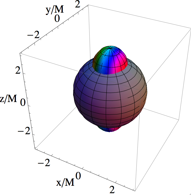
Figure 8: Shape of regions where $E=B$ in Kerr-Schild metric for $\beta_{0}=0.5$; compare with Fig. 3.

References

- Armitage and Natarajan (2002) P. J. Armitage and P. Natarajan, ApJ Lett. 567, L9 (2002), eprint arXiv:astro-ph/0201318.
- Krolik (2010) J. H. Krolik, Astrophys. J. 709, 774 (2010), eprint 0911.5711.
- Milosavljević and Phinney (2005) M. Milosavljević and E. S. Phinney, ApJ Lett. 622, L93 (2005), eprint arXiv:astro-ph/0410343.
- van Meter et al. (2010) J. R. van Meter, J. H. Wise, M. C. Miller, C. S. Reynolds, J. Centrella, J. G. Baker, W. D. Boggs, B. J. Kelly, and S. T. McWilliams, ApJ Lett. 711, L89 (2010), eprint 0908.0023.
- Blandford and Znajek (1977) R. D. Blandford and R. L. Znajek, MNRAS 179, 433 (1977).
- Lyutikov (2010) M. Lyutikov, ArXiv e-prints (2010), eprint 1010.6254.
- Goldreich and Lynden-Bell (1969) P. Goldreich and D. Lynden-Bell, Astrophys. J. 156, 59 (1969).
- McWilliams (2010) S. T. McWilliams, ArXiv e-prints (2010), eprint 1012.2872.
- Palenzuela et al. (2010a) C. Palenzuela, T. Garrett, L. Lehner, and S. L. Liebling, Phys. Rev. D 82, 044045 (2010a), eprint 1007.1198.
- Palenzuela et al. (2010b) C. Palenzuela, L. Lehner, and S. L. Liebling, Science 329, 927 (2010b), eprint 1005.1067.
- Neilsen et al. (2010) D. Neilsen, L. Lehner, C. Palenzuela, E. W. Hirschmann, S. L. Liebling, P. M. Motl, and T. Garret, ArXiv e-prints (2010), eprint 1012.5661.
- Wald (1974) R. M. Wald, Phys. Rev. D 10, 1680 (1974).
- Hanni and Ruffini (1976) R. S. Hanni and R. Ruffini, Nuovo Cimento Lettere 15, 189 (1976).
- Ernst (1976) F. J. Ernst, Journal of Mathematical Physics 17, 54 (1976).
- Beskin (1997) V. S. Beskin, Soviet Physics Uspekhi 40, 659 (1997).
- Thorne et al. (1986) K. S. Thorne, R. H. Price, and D. A. MacDonald, Black holes: The membrane paradigm (Black Holes: The Membrane Paradigm, 1986).
- Linet (1976) B. Linet, Journal of Physics A Mathematical General 9, 1081 (1976).
- Goldreich and Julian (1969) P. Goldreich and W. H. Julian, Astrophys. J. 157, 869 (1969).
- Michel (1979) F. C. Michel, Astrophys. J. 227, 579 (1979).
- Smith et al. (2001) I. A. Smith, F. C. Michel, and P. D. Thacker, MNRAS 322, 209 (2001).
- Pétri et al. (2002) J. Pétri, J. Heyvaerts, and S. Bonazzola, AAP 387, 520 (2002).
- Spitkovsky (2006) A. Spitkovsky, ApJ Lett. 648, L51 (2006), eprint arXiv:astro-ph/0603147.
- Arons and Scharlemann (1979) J. Arons and E. T. Scharlemann, Astrophys. J. 231, 854 (1979).
- Hibschman and Arons (2001) J. A. Hibschman and J. Arons, Astrophys. J. 554, 624 (2001), eprint arXiv:astro-ph/0102175.
- Balbus and Hawley (1991) S. A. Balbus and J. F. Hawley, Astrophys. J. 376, 214 (1991).
- O’Neill et al. (2009) S. M. O’Neill, M. C. Miller, T. Bogdanović, C. S. Reynolds, and J. D. Schnittman, Astrophys. J. 700, 859 (2009), eprint 0812.4874.
- Cheng et al. (1986) K. S. Cheng, C. Ho, and M. Ruderman, Astrophys. J. 300, 500 (1986).
- Abdo et al. (2010) A. A. Abdo, M. Ackermann, M. Ajello, W. B. Atwood, M. Axelsson, L. Baldini, J. Ballet, G. Barbiellini, M. G. Baring, D. Bastieri, et al., Astrophys. J. Suppl. 187, 460 (2010), eprint 0910.1608.
- Hirotani et al. (2003) K. Hirotani, A. K. Harding, and S. Shibata, Astrophys. J. 591, 334 (2003), eprint arXiv:astro-ph/0212043.
- Lyutikov et al. (1999) M. Lyutikov, R. D. Blandford, and G. Machabeli, MNRAS 305, 338 (1999), eprint astro-ph/9806363.
- Melrose and Gedalin (1999) D. B. Melrose and M. E. Gedalin, Astrophys. J. 521, 351 (1999).
- Gruzinov (1999) A. Gruzinov, ArXiv Astrophysics e-prints (1999), eprint astro-ph/9902288.
- ’t Hooft (1976) G. ’t Hooft, Physical Review Letters 37, 8 (1976).
- Rubakov and Shaposhnikov (1996) V. A. Rubakov and M. E. Shaposhnikov, Soviet Physics Uspekhi 39, 461 (1996), eprint arXiv:hep-ph/9603208.