Sparse Partitioning: Nonlinear regression with binary or tertiary predictors, with application to association studies

Abstract

This paper presents Sparse Partitioning, a Bayesian method for identifying predictors that either individually or in combination with others affect a response variable. The method is designed for regression problems involving binary or tertiary predictors and allows the number of predictors to exceed the size of the sample, two properties which make it well suited for association studies.

Sparse Partitioning differs from other regression methods by placing no restrictions on how the predictors may influence the response. To compensate for this generality, Sparse Partitioning implements a novel way of exploring the model space. It searches for high posterior probability partitions of the predictor set, where each partition defines groups of predictors that jointly influence the response.

The result is a robust method that requires no prior knowledge of the true predictor–response relationship. Testing on simulated data suggests Sparse Partitioning will typically match the performance of an existing method on a data set which obeys the existing method’s model assumptions. When these assumptions are violated, Sparse Partitioning will generally offer superior performance.

and

tt1Supported by an EPSRC doctoral fellowship. t2Supported in part by NIH ENDGAME Grant U01 HL084706 and NIH Grant P50 HG02790.

Introduction

In recent years association studies have surged in popularity, driven by the ability to interrogate the genome in ever-increasing detail [McCarthy et al. (2008)]. The common aim of these studies is to detect genomic variants that are linked with a particular phenotype. It is hoped that detecting such variants will bring us closer to understanding the biological processes at work.

So far these studies have had mixed results. While variants with strong effects are picked up fairly readily [e.g., The Wellcome Trust Case Control Consortium (2007)], there is speculation that more subtle associations are being missed [Cordell (2009)]. This suggests the need to develop more sophisticated tools that are able to explore beyond the obvious [Stephens and Balding (2009)].

Formally, an association study can be viewed as a regression problem consisting of $n$ data points (the samples) and $N$ predictors (the variants). In this paper we consider the case when each predictor takes either two or three unique values. This is common in association studies. For example, a predictor might record presence or absence of a mutation, or whether a variant is in a neutral, amplified or deleted state. We also allow for “large $p$, small $n$ problems” in which the number of predictors exceeds the sample size. Again, this is often the case with association studies, owing to the abundance of genetic variants available to examine.

Currently available regression tools can be characterized by how they permit predictors to influence the response. For example, many fit an additive model, which overlooks the possibility that interactions between predictors might affect the response. The methods which permit interactions will generally specify the type of interactions they allow. A key factor affecting performance is whether the data set being examined conforms to the restrictions the method imposes. Sparse Partitioning tries to avoid placing restrictions on the underlying model relationship. This should enable it to maintain power in scenarios where other methods might fail.

Section 1 describes some of the existing methods suitable for processing high-dimensional data. Sections 2 and 3 briefly outline the Sparse Partitioning methodology. Sections 4 and 5 test the performance of Sparse Partitioning compared to existing methods, while Section 6 concludes the paper. Additional details are provided in the Appendix and supplementary material.

1 Existing methods

The task of a regression method is to infer how the predictors influence the response. Let the vector $\mathbf{Y}$ (size $n\times 1$) contain the response values and the matrix $\mathbf{X}$ (size $n\times N$) contain the predictors. For the $i$th data point, $Y_{i}$ denotes its response, while $X_{i,1},\ldots,X_{i,g},\ldots,X_{i,N}$ denote its predictor values. If we write the regression model as $l(\mathbb{E}(\mathbf{Y}))=f(\mathbf{X})$, where $l$ is a specified link function, the aim is to deduce properties of $f(\mathbf{X})$, the “underlying relationship.” In particular, we wish to identify the subset of predictors that contribute toward $f(\mathbf{X})$.

Consider writing the underlying relationship as

$$f(\mathbf{X})=f_{1}(X_{G_{1,1}},\ldots,X_{G_{1,s_{1}}})+\cdots+f_{K}(X_{G_{K,1}},\ldots,X_{G_{K,s_{K}}}).$$

Under this representation, $f(\mathbf{X})$ is influenced by additive contributions from groups of interacting predictors. $f_{k}$ describes the contribution of predictors $G_{k,1},\ldots,G_{k,j},\ldots,G_{k,s_{k}}$ to $f(\mathbf{X})$. In this paper, additivity is not considered an interaction. Therefore, the predictors in each group are said to interact with each other, but not to interact with a predictor in a different group. For the most general relationship, all predictors feature in one group. In practice, however, we suspect $f(\mathbf{X})$ is far simpler.

We have distinguished existing methods based on two features of their underlying relationships: whether they permit more than one group of predictors to contribute to $f(\mathbf{X})$ and whether they permit interactions between contributing predictors. Figure 1 demonstrates the four possibilities, using the case when the predictors are binary and the response is continuous.

1.1 One group, maximum group size one

$$f(\mathbf{X})=f_{1}(X_{G_{1,1}}).\vspace*{-2pt}$$

The simplest assumption supposes the response is influenced by only one predictor. Most methods in this category are equivalent to performing a maximum likelihood test comparing a null hypothesis, $f(\mathbf{X})=$ constant, with an alternative, $f(\mathbf{X})=f_{1}(X_{g})$. Single is our implementation of such a method. Considering that these methods can only detect an associated predictor by its marginal effect, they are surprisingly successful. They are also extremely fast to run and therefore very popular [e.g., Stranger et al. (2007)].

		ONE GROUP		MULTIPLE GROUPS
		OF PREDICTORS		OF PREDICTORS
NO INTERACTIONS		$\mathbf{Y}=\alpha+\beta X_{g}$ e.g., Single		$\mathbf{Y}=\alpha+\sum_{1}^{N}\beta_{g}X_{g}$ e.g., SSS
INTERACTIONS		$\mathbf{Y}=f(X_{G_{1}},\ldots,X_{G_{s}})$ e.g., Pairs, CART, RF		$\mathbf{Y}=f_{1}(X_{G_{1,1}},\ldots,X_{G_{1,s_{1}}})+\cdots+$ $f_{K}(X_{G_{K,1}},\ldots,X_{G_{K,s_{K}}})$ e.g., Logic, MARS, Sparse Partitioning

Figure 1: Regression methods can be categorized according to two features of their underlying relationship. This table shows the four possibilities, for the case of binary predictors and a continuous response. Explanations of the existing methods, Single, Pairs, CART, RF, SSS, Logic and MARS, are provided in the main text.

Bayesian alternatives are possible [e.g., Balding (2006)] and useful if certain predictors are thought a priori more likely to be associated. Otherwise they will generally produce the same results as classical methods.

1.2 One group, maximum group size greater than one

$$f(\mathbf{X})=f_{1}(X_{G_{1,1}},\ldots,X_{G_{1,{s_{1}}}}).\vspace*{-2pt}$$

Even for very high-dimensional problems ($>$500,000 predictors) it is possible to test exhaustively all pairwise models [cf. Marchini, Donnelly and Cardon (2005)]. The method Pairs is our extension of Single, performing a maximum likelihood test for each pair of predictors. While the method could be extended further to consider three or four way interactions, this is often infeasible due to computation time.

A second method in this category is CART [Classification and Regression Trees; Breiman et al. (1984)]. CART differs from Pairs in not insisting on the full interaction model for associated predictors. For example, a CART model containing two associated predictors might have only 3 degrees of freedom, even though there are 4 unique vector values present. Random Forest [Breiman (2004)] offers a stochastic interpretation of this method, constructing a large number of trees in a quasi-random fashion and summarizing their properties.

1.3 More than one group, maximum group size one

$$f(\mathbf{X})=f_{1}(X_{G_{1,1}})+\cdots+f_{K}(X_{G_{K,1}}).\vspace*{-2pt}$$

This underlying relationship allows more than one predictor to be causal, but restricts the causal predictors to contributing additively. When there are more predictors than samples, the standard multiple regression model will become over-saturated and fail.

The classical solution, adopted by Variable Subset Selection, Lasso and Ridge Regression [described in Hastie, Tibshirani and Friedman (2001)], is to introduce a penalty term that limits the number of contributing predictors. However, this penalty term can appear quite arbitrary. An alternative is offered by Bayesian methods [Wang et al. (2005); Zhang et al. (2005); Hoggart et al. (2008)]. These methods allow our preference for sparse models to be reflected in the prior distribution. We picked Shotgun Stochastic Search [Hans, Dobra and West (2007)] to represent this category of methods in the simulation studies.

1.4 More than one group, maximum group size greater than one

$$f(\mathbf{X})=f_{1}(X_{G_{1,1}},\ldots,X_{G_{1,s_{1}}})+\cdots+f_{K}(X_{G_{K,1}},\ldots,X_{G_{K,s_{K}}}).\vspace*{-2pt}$$

Allowing both interactions and multiple groups of predictors to contribute to the underlying relationship has the potential of most accurately describing the true model. However, both decisions increase the size of the model space and so the difficulty of identifying the true model.

Logic Regression [Ruczinski, Kooperberg and LeBlanc (2003)] and Multivariate Adaptive Regression Splines are two of the few methods in this class. Both methods place restrictions on the permitted functions which reduce the size of the model space; Logic insists on Boolean operators, while MARS uses products of hinge functions. Sparse Partitioning falls into this category, but places no restriction on the types of functions allowed.

2 Formulating the regression as a partitioning

In order to describe Sparse Partitioning’s methodology, it is convenient to formulate the regression problem as a search for high scoring partitions. Consider how the underlying relationship groups predictors:

$$f(\mathbf{X}) = f_{1}(X_{G_{1,1}},\ldots,X_{G_{1,s_{1}}})+\cdots+f_{K}(X_{G_{K,1}},\ldots,X_{G_{K,s_{K}}})$$

$$= f_{1}({X}_{\mathbf{G}_{1}})+\cdots+f_{K}({X}_{\mathbf{G}_{K}}).\vspace*{-2pt}$$

The disjoint sets $\mathbf{G}_{1},\mathbf{G}_{2},\ldots,\mathbf{G}_{K}$ index groups of associated predictors. If we let $\mathbf{G}_{0}$ index the “null group”—the group of predictors in no way associated with the response—then $\mathbb{G}=\{\mathbf{G}_{0},\mathbf{G}_{1},\mathbf{G}_{2},\ldots,\mathbf{G}_{K}\}$ defines a partitioning of $\{1,2,\ldots,N\}$.

In the representation above, predictors are not allowed to feature in more than one nonnull group. To avoid this restriction, while at the same time maintaining a partitioning, the predictor set is expanded to contain $C$ copies of each predictor and $N$ is increased accordingly. For the remainder of this paper, we describe the method supposing $C=1$, then explain the changes required when this is not the case.

A partition can also be described by the vector $\mathbf{I}=(I_{1},I_{2},\ldots,I_{N})$, where $I_{g}$ indicates to which group predictor $g$ belongs. This notation will be useful later on and also reminds us that the ordering within groups is not important. Figure 2 gives an example of a simple partitioning and the underlying relationship to which it refers.

$\mathbf{I}$ $=$ $(\overbrace{11}^{\mathbf{G}_{1}}\overbrace{00}^{\mathbf{G}_{0}}\overbrace{2}^{\mathbf{G}_{2}})$ $f(\mathbf{X})$ $=$ $f_{1}(X_{1},X_{2})+f_{2}(X_{5})$

$\Rightarrow$

For binary predictors and a continuous response: $\mathbf{Y}=\alpha_{0}+\alpha_{1,1}X_{1}(1-X_{2})+\alpha_{1,2}(1-X_{1})X_{2}$ $+\,\alpha_{1,3}X_{1}X_{2}+\alpha_{2,1}X_{5}$$\alpha_{1,2}(1\,X_{1})X_{2}$

Figure 2: An example of a partitioning for a problem containing five binary predictors (each valued 0 or 1) and a continuous response.

The focus of Sparse Partitioning is to determine properties of the partitioning defined by the underlying relationship. Our main desire is to identify which predictors are not in the null group. However, it is also useful to know whether predictors feature in the same nonnull group, indicating interactions. The advantage of formulating the problem in terms of partitions is that the model space is likely too vast to hope to detect accurately the explicit underlying relationship (i.e., determine $\mathbf{f}=\{f_{1},f_{2},\ldots,f_{K}\}$ as well as $\mathbb{G}$). Fortunately, we are usually more interested in detecting which predictors are involved, rather than exactly how they contribute (the latter can be saved for follow-up analysis).

3 Sparse Partitioning methodology

Sparse Partitioning is a Bayesian methodology, so it follows the usual steps of deciding a prior, calculating the likelihood, then computing the posterior distribution of models through use of Bayes formula:

$$\mathbb{P}(\mathrm{Model}|\mathrm{Data})\propto\mathbb{P}(\mathrm{Model})\times\mathbb{P}(\mathrm{Data}|\mathrm{Model}).$$

Each model is defined by $\{\mathbb{G},\mathbf{f}\}$, a partition and a corresponding set of functions. However, $\mathbf{f}$ is considered a nuisance parameter, so we are interested in determining the marginal posterior $\mathbb{P}(\mathbb{G}|\mathrm{Data})$.

3.1 Prior

$$\mathbb{P}(\mathrm{Model})=\mathbb{P}(\mathbb{G},\mathbf{f})=\mathbb{P}(\mathbb{G})\times\mathbb{P}(\mathbf{f}|\mathbb{G}).\vspace*{-2pt}$$

The prior for the partition is based on our belief in $p_{g}$, the probability that predictor $g$ is associated with the response. Therefore, $\mathbb{P}(\mathbb{G})=\mathbb{P}(\mathbf{I})$ is constructed such that $\sum_{\mathbf{I}:I_{g}\neq 0}\mathbb{P}(\mathbf{I})=p_{g}$. Two partitions containing the same associations are given equal weight. When multiple copies of each predictor are permitted, $p_{g}$ equals the probability that at least one copy of predictor $g$ is associated. Sparse Partitioning keeps fixed the values of $p_{g}$, however, it is straightforward to allow them to vary if more detailed prior information is available.

Given $\mathbf{G}_{k}$, the relevant information of function $f_{k}$ can be described by the values it assigns each node (unique vector value) of $X_{\mathbf{G}_{k}}$. For the example in Figure 2, $\mathbf{f}$ can be described by $\bolds{\alpha}=(\alpha_{0},\alpha_{1,1},\alpha_{1,2},\alpha_{1,3},\alpha_{2,1})$. Therefore, the prior on $\mathbf{f}$ is equivalent to a prior on $\bolds{\alpha}$, for which Sparse Partitioning uses a multivariate normal distribution.

3.2 Likelihood

The likelihood is determined by the regression model. When the response is continuous (e.g., a quantitative trait), Sparse Partitioning supposes the residuals are normally distributed. When the response is binary (e.g., a case-control experiment with affected and unaffected patients), Sparse Partitioning uses a logit link function. The marginal likelihood is obtained by integrating across the function parameters:

$$\mathbb{P}(\mathrm{Data}|\mathbb{G})=\int_{\mathbf{f}}\mathbb{P}(\mathrm{Data}|\mathbf{f},\mathbb{G})\mathbb{P}(\mathbf{f}|\mathbb{G})\,d\mathbf{f}=\int_{\bolds{\alpha}}\mathbb{P}(\mathrm{Data}|\bolds\alpha,\mathbb{G})\mathbb{P}(\bolds\alpha|\mathbb{G})\,d\bolds{\alpha}.\vspace*{-2pt}$$

3.3 Posterior

Explicit calculation of $\mathbb{P}(\mathbb{G}|\mathrm{Data})$ would require an exhaustive search of the space of partitions, which is infeasible even for reasonably sized problems. Therefore, Sparse Partitioning uses Markov Chain Monte Carlo (MCMC) techniques to estimate statistics of this posterior distribution. Within each MCMC iteration, two sampling stages are used: the first proposes, in turn, a change to each component of $\mathbf{I}$; the second proposes a change to one element of $\mathbb{G}$. The bulk of Sparse Partitioning’s processing time is spent sampling from the posterior distribution. Therefore, it is convenient that the two stages can be parallelized with an almost linear speed-up.

Full details of the methodology are provided in Appendix and Sections 1, 2 and 3 of the Supplementary Material [Speed and Tavaré (2010)].

4 Simulation studies

In total, ten simulation studies were carried out, designed to test various aspects of Sparse Partitioning’s performance and make comparisons with existing methods. This section presents results from the first study. Further details of the methods used to simulate data and the results from the remaining nine studies are provided in Section 4 of the Supplementary Material [Speed and Tavaré (2010)].

Typically, each simulated data set consisted of 100 samples, each of 1000 predictors, three of which were causal for the response. Each regression method was asked to identify its top three associations and was then scored by how many causal predictors it correctly identified. Empirical estimates were obtained by averaging over 100 data sets.

The first study examined the case of (uncorrelated) binary predictors and a continuous response. Each scenario concentrated on a particular underlying relationship (Models I, II or III) for a particular frequency of the causal predictors (0.05, 0.1, 0.2, 0.4 or random). The first model was designed so that each causal predictor contributed additively, the second featured a multiplicative interaction, while the third involved a “weird” interaction (see Table 1).

Table 1: The first simulation study considered three different underlying relationships

Model	Underlying relationship
I	$Y=X_{1}+1.5X_{2}-2X_{3}$
II	$Y=1.5X_{1}\times X_{2}+X_{3}$
III	$Y=f(X_{1},X_{2})+X_{3};$
	$f(0,0)=0$, $f(1,0)=1$, $f(0,1)=2$, $f(1,1)=-1$

Figure 3 presents results from the first study. Each plot relates to a different underlying relationship. Within each plot, the lines display the average number of causal predictors correctly identified by each method for different frequencies of the causal predictors. Figure 4 provides an alternative interpretation of these results, reporting how often each method successfully detected 0, 1, 2 or 3 causal predictors for each scenario.

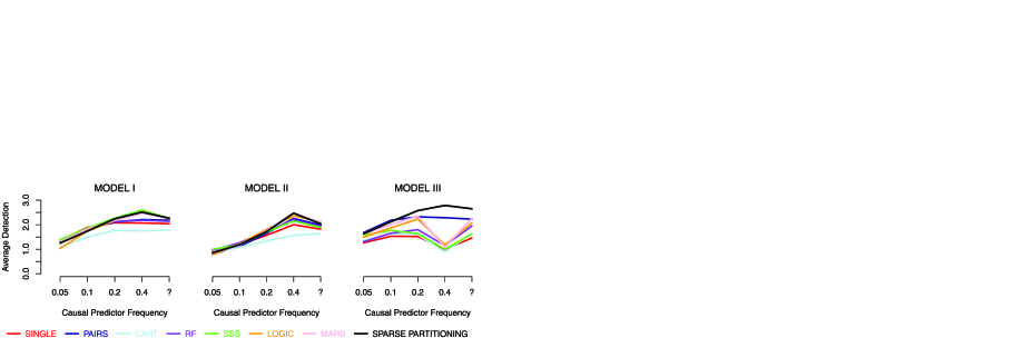
Figure 3: Each plot considers a different underlying relationship (described in the main text). Within each plot, the lines report the average number of causal predictors correctly detected by each method for different causal predictor frequencies (“?” denotes random).

Under Model I, SSS, Logic, MARS and Sparse Partitioning were the four best performing methods across different frequencies, pulling clear of Single, Pairs and RF as the causal predictor frequency increased. Under Model II, this order was essentially maintained, with the exception of SSS, which dropped into the second tier of performers. However, under Model III, Sparse Partitioning has emerged on top, comprehensively beating six of its rivals, with only Pairs coming close.

Sparse Partitioning has performed best in this simulation study, proving itself most robust across the different models. It has triumphed under Model III, when the underlying relationship assumptions of all other methods have been violated. Note that its generality has not prevented it from at least matching the performance of the existing methods under Models I and II.

Figure 4: Each group of eight vertical bars compares the methods for a particular underlying relationship and causal predictor frequency (“?” denotes random). Within each bar, the lengths of the shaded sections (from top to bottom) indicate the proportion of time the method correctly detected 0, 1, 2 and 3 causal predictors. For example, the lengths of the darkest gray bars show how often each method successfully identified all three causal predictors. For all scenarios, the ordering of methods is the same (from left to right): Single, Pairs, CART, RF, SSS, Logic, MARS and Sparse Partitioning.

5 Application to real data sets

We applied Sparse Partitioning to four previously analyzed association studies: the first looked at expression data for 109 individuals in the HapMap project (http://hapmap.ncbi.nlm.nih.gov); the second and third examined data sets from the “2010 Project” (http:// walnut.usc.edu/2010), a large-scale study of the plant Arabidopsis thaliana; the fourth used data provided by the Flint laboratory at the University of Oxford (http://www.well.ox.ac.uk/flint-2). Extended versions of all results are provided in Figures 12–16 of the Supplementary Material [Speed and Tavaré (2010)].

5.1 HapMap data

Dr. Antigone Dimas kindly provided us with a sample of 109 individuals, each typed for 1,186,075 Single Nucleotide Polymorphisms (SNPs) and measured for expression levels of 2682 genes [Dimas (2009)]. We applied Sparse Partitioning to the four genes for which Dr. Dimas found strongest evidence for an interaction, copying her decision to consider only SNPs within one million base pairs (1 Mbp) of each gene. Figure 5 presents the results for MTHFR, the third of these genes, located approximately 11.8 Mbp along Chromosome 1. For each SNP in the 2 Mbp region, the top plot displays the $p$-value obtained by Single, while the bottom plot reports the posterior probability of association from Sparse Partitioning (circles correspond to run one result, triangles to run two). The solid vertical line marks the location of the gene, while the two dashed vertical lines mark the locations of the SNPs declared interacting by Dr. Dimas. The dashed horizontal lines provide estimates of the 5, 25 and 50% significance thresholds for the top association of each method, calculated using permutation tests.

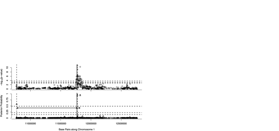
Figure 5: Analysis of expression levels of MTHFR using HapMap data. The top plot shows results from Single, the bottom plot shows results from two runs of Sparse Partitioning. Full details are provided in the main text.

Sparse Partitioning found three promising SNPs, rs2286139, rs2643888 and rs2279703, with posterior probabilities of association 0.57, 0.96 and 0.96, respectively. It is no coincidence that the second and third hits have matching probabilities. Before analysis, Sparse Partitioning searches for highly correlated predictors, as is often the case with fine-scale genetic data. SNP rs2643888 was found to be highly correlated with SNP rs2279703, with matching values for 106 of the 109 individuals. Therefore, the former SNP was removed from analysis, and subsequently given the same posterior estimates as the latter. Sparse Partitioning returned a posterior probability of interaction of 0.42 between SNPs rs2286139 and rs2643888/rs2279703 (indicated by the horizontal arrows), offering some support for Dr. Dimas’ findings of an interaction.

5.2 2010 project: Pilot data

The project’s pilot data set looked at 95 accessions, genotyped for 5419 SNPs and measured for ten phenotypic traits. We focused on the tenth phenotype, expression levels of the FRIGIDA gene. We decided to remove eight accessions whose genotypes were either almost identical to remaining accessions or were flagged as suspicious by principal component analysis. Using methods similar to the original analysis [Zhao et al. (2007)], we first adjusted the phenotype to correct for confounding due to population structure and relatedness of accessions. By contrast, we chose not to impute missing values, meaning approximately 10% of the genotypes were supplied to Sparse Partitioning as unobserved.

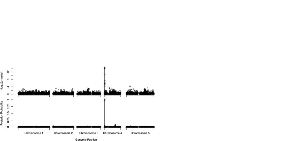
Figure 6: Analysis of expression levels of FRIGIDA for Arabidopsis thaliana. The top plot shows results from Single, the bottom plot shows results from two runs of Sparse Partitioning. Full details are provided in the main text.

Figure 6 compares the $p$-values obtained from Single to the posterior probabilities of association of Sparse Partitioning. Our method identified just one strong association, coinciding with the third strongest hit of Single and suggesting that, in this case, the simple underlying relationship of Single might be appropriate. For both methods the strong associations lay very close to the FRIGIDA region, marked by a solid vertical line, suggesting the results are accurate.

A possible concern is that Sparse Partitioning’s generality might lead to overfitting on occasions when simple models are more appropriate. Here that does not appear to be the case, with Sparse Partitioning declaring only one strong association. We repeated the analysis using imputed data, which allowed us to compare the prediction accuracy of each method via leave-one-out cross-validation. The linear model containing only the top hit from Single explained 44% of the variance, agreeing closely with Sparse Partitioning’s estimate of 42% variance explained.

5.3 2010 project: Release 3.04

We examined how Sparse Partitioning would deal with a problem encountered in the 2010 project’s most recent paper [Atwell et al. (2010)]. The expression level of the FLC gene is known to be affected by polymorphisms in the FRIGIDA region [Johanson et al. (2000); Shindo et al. (2005)]. Atwell et al. performed a one-SNP-at-a-time association study using FLC expression as the response. Its analysis produced results similar to our analysis by Single, shown in the top plot of Figure 7. While some SNPs within the FRIGIDA region (which is marked by a vertical line) achieved genome-wide significance, two stronger groups of associations were detected approximately 200 kbp and 1 Mbp to the right. Prior knowledge would suggest these downstream associations are spurious. When Atwell et al. repeated the analysis, but this time including in the regression model two alleles of the FRIGIDA gene known to affect FLC, the downstream associations vanished, increasing suspicion that they were false positives. For the rest of this section, we assume this to be the case.

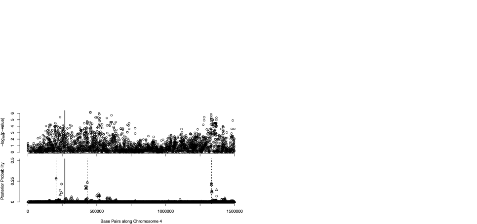
Figure 7: Analysis of expression levels of FLC for Arabidopsis thaliana. The top plot shows results from Single, the bottom plot, which has a truncated $y$-axis, shows results from two runs of Sparse Partitioning. Full details are provided in the main text.

The project’s latest data release provides typing for 214,553 SNPs across five chromosomes. We picked the 3509 SNPs located within the first 1.5 Mbp of Chromosome 4. As this subset was a biased selection (e.g., it contained over two-thirds of those SNPs with marginal $p$-values less than $10^{-4}$), it was necessary to reflect this when choosing the prior probability of association for Sparse Partitioning. In the event, we settled upon a prior probability of 1 in 3500.

We used imputed data for this analysis, as the increased SNP density allowed missing values to be inferred more reliably. Similar to the analysis of Atwell et al., we decided to correct only for relatedness, as discussions with members of the Nordborg group convinced us that adjusting for population structure risked removing too much true signal. The bottom plot of Figure 7 shows the results of Sparse Partitioning. The dashed vertical lines indicate the three regions where our method found most evidence of association. While two false positives remained, Sparse Partitioning gave greatest recognition to the FRIGIDA region, identifying a possible association approximately 60 kbp upstream of the gene.

In this example, we had knowledge of the true causal region, allowing us to identify the false associations. The concern is that this example is one of many, and that most times we will not know the correct answer. In these cases, the best we can hope is that a method acknowledges the true and false positives, but recognizes the uncertainty. This is what Sparse Partitioning has done here. Furthermore, our method more precisely identified peaks than Single which should speed up the verification process.

5.4 Mouse data

Jon Krohn, from Professor Jonathan Flint’s group at the University of Oxford, kindly provided us with CD4 counts for 1274 “heterogeneous stock” mice [Solberg et al. (2006)], along with genotypic values for 770 SNPs covering the length of Chromosome 5. Krohn had previously analyzed this data set using Bagphenotype, software designed by Dr. William Valdar (http://www.unc.edu/~wvaldar/bagphenotype.html). The response values were continuous, while the predictors were tertiary. Only a tiny proportion of genotypes (0.1%) were missing, so we saw no need to impute values and instead left them as unobserved. In addition, we were provided with the gender of each mouse, which we coded as a binary variable and included in the set of predictors.

As the chromosomal region was a subsection of a genome-wide study, we decided a prior probability of association of 1 in 10,000 was appropriate for each SNP. There is overwhelming prior knowledge that CD4 counts are linked to gender [e.g., Maini et al. (1996)], so we decided upon a prior probability of 0.5. We run Sparse Partitioning allowing three copies of each predictor ($C=3$). As Figure 8 demonstrates, the top hits from Single, SNPs CEL-5_106584673 and rs13478460, which due to linkage disequilibrium are almost identical, persisted in Sparse Partitioning. In addition, our method declares associated SNP rs13478156. As indicated by the horizontal arrows, Sparse Partitioning found evidence of interactions between gender and the top SNPs. To test the effect of our prior choices, we repeated the analysis with prior probabilities {$10^{-4}$, 0.1}, {$10^{-3}$, 0.5} and {$10^{-3}$, 0.1}, and obtained very similar results on each occasion (results not shown).

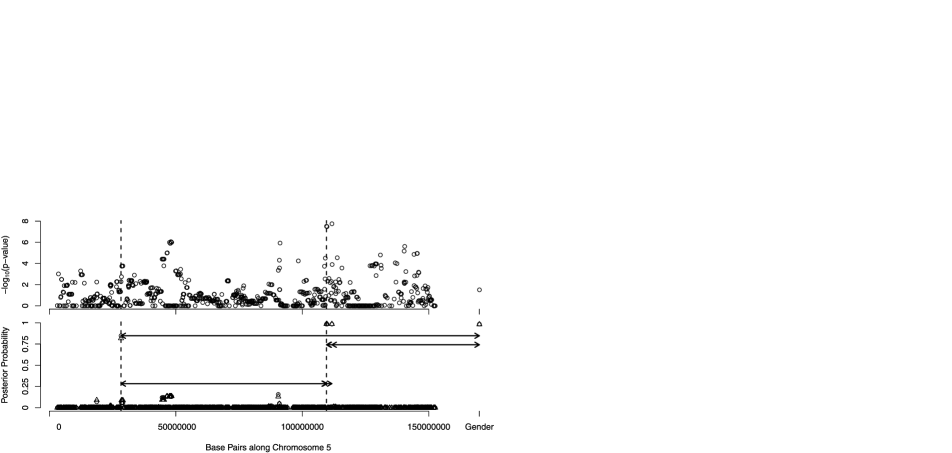
Figure 8: Analysis of CD4 count in mice. The top plot shows results from Single, the bottom plot shows results from two runs of Sparse Partitioning. Full details are provided in the main text.

Maximum likelihood tests offer justification for why rs13478156 was found by Sparse Partitioning, but largely overlooked by Single. The supplementary material provides plots for two sets of tests. The first set compares, for each SNP, the pairwise interaction with gender against a null model of no association. We find that the top hits of Single remain the most significant hits here. However, these tests provide only limited information about the strength of the interaction terms. Therefore, the second set compares the pairwise interaction model against the additive model for that SNP and gender. We see that the interaction between rs13478156 and gender is highly significant. This supports Sparse Partitioning’s claim that this SNP acts in a gender specific way, which also agrees with findings from Krohn’s analysis.

This data set demonstrated the advantage of allowing multiple copies of each predictor. When Sparse Partitioning is run without this option (results for $C=1$ are shown in the supplementary material), the best fitting partition features three associated predictors in a single nonnull group. The posterior estimates of pairwise interactions cannot be trusted because the method is unable to distinguish between, say, a single three-way interaction and a pair of two-way interactions. Allowing multiple copies of predictors requires only a small increase in computation time, so we recommend this option is used.

6 Discussion

It is fairly easy to design a regression method that is finely tuned for a specific underlying relationship and then demonstrate its superior power on data sets which obey this model. If one were presented only with the results of the Model III simulations, it would be easy to think that Sparse Partitioning is such a method. We have tried to show this is not case. We believe that Sparse Partitioning offers a robust alternative to existing methods. It fares equally well under simple models, but comes into its own as the model becomes more complex.

6.1 Prospects for nonlinear regression

Nonlinear regression methods are competing over a fairly small share of the market, bounded on the one side by the performance of methods such as Single and on the other by the strength of signal present in the data. Despite these limitations, there remains a demand for such methods. There are many examples where standard linear methods fail to explain a satisfactory percent of the variation, so it is quite possible that nonadditive systems are at work. Sparse Partitioning should not be viewed as a search for interactions, but rather as a regression method which bears interactions in mind. Even for situations in which it cannot pinpoint an interaction with certainty, its detection power should benefit for having considered their existence.

6.2 Generality

Sparse Partitioning’s strength derives from the generality of its underlying relationship. Therefore, it is perhaps a surprise that the method does not appear to suffer in situations where this relationship is overly complicated. The results in Section 4 suggest there is no inherent disadvantage to using such a general underlying relationship. While Sparse Partitioning will almost certainly overfit the true model at some points in the MCMC sampling, its posterior estimates are based on model averages, rather than the single highest scoring model visited. For this reason, it should not matter if a nonassociated predictor is occasionally declared associated, as these errors are likely to be spread thinly across the noncausal predictors. Additionally, as Sparse Partitioning seeks only to estimate marginal posterior probabilities, using an underlying relationship too general should not upset the Bayesian mechanics. The prior probability that a predictor is associated remains constant (equal to $p_{g}$) regardless of the size of the model space. Even if excessive generality does affect some aspects of the posterior distribution, the marginal posterior probabilities should remain correct.

6.3 Diagnosis

The only way to calculate the posterior distribution exactly is through an exhaustive search of the space of partitions. Unfortunately, this is feasible for only the smallest data sets, so instead Sparse Partitioning is forced to explore the model space in a stepwise fashion. In this respect, Sparse Partitioning’s search holds an advantage over deterministic algorithms. When deciding which model in the neighborhood to visit next, Sparse Partitioning is not forced to move to the highest scoring model. Instead it is able to try a lower scoring move, in the hope that this is a gateway to a higher scoring region.

The drawback of this stochasticity is the variability it introduces into Sparse Partitioning’s results. The analysis in Section 5 provides some tips for gauging Sparse Partitioning’s performance. It is sensible to compare the results with those of Single, as we would expect very strong associations to be found by both methods. Repeating the analysis with a new random seed will highlight obvious lack of convergence, as should examination of trace plots. Additionally, if time permits, repeating the analysis with the response values permuted will provide significance thresholds under a model of no true associations.

6.4 Limitations

The processing time required for each iteration scales linearly with $N$. We speculate that the number of iterations required for convergence scales approximately with the 1.5th power of $N$ (based on the stepwise nature of Sparse Partitioning’s search) and exponentially with the number of true associations (based on the growth of the model space).

As a rule of thumb, we consider Sparse Partitioning suitable for problems with no more than 20,000 predictors, or cases where $N/n<100$. This is not to say that Sparse Partitioning cannot be applied on, say, a genome-wide scale, but it may be necessary to filter the predictors first. We suggest picking, for example, the highest 10% of hits from Single. Of course, this is not ideal. It is certainly possible that true associations are concealed within the remaining 90% of predictors. But considering standard practice involves picking, perhaps, the top 100 hits of Single for further analysis, the ability to consider instead the top few thousand hits should offer a significant advantage. As we experienced in Section 5, it is important to realize when we have selected a biased subset of predictors and reflect this in the prior probability of association. The easiest solution is to pick the priors as if analyzing the complete set of predictors.

We have identified situations in which Sparse Partitioning will struggle. Examples were found in Simulation Studies Five and Ten (see Supplementary Material). The latter was an almost unavoidable situation because the true relationship heavily contradicted our prior beliefs. The former demonstrated the drawback of treating tertiary predictors as categorical variables, when in fact their values have a natural ordering. We suspect that this problem can be overcome by application of a Bayesian version of Projection Pursuit [described in Hastie, Tibshirani and Friedman (2001)] that we are now developing.

Additionally, consider the case in which the response is influenced by an interaction of two predictors, but the inclusion of neither predictor on its own significantly improves the model fit. For one of these predictors to have a realistic chance of being included in a nonnull group, the improvement in fit must offset the penalty of inclusion implied by $\mathbb{P}(\mathbb{G})$. Because of the single-step nature of Sparse Partitioning’s search, it is unlikely that either predictor will appear in the current model, which is required for the method to consider their interaction. For our method to be successful in this case, it would have to permit two-step moves or resort to an exhaustive search.

Sparse Partitioning can be used when the predictors are continuous, provided a suitable transformation exists. For example, we have applied our method to copy number values, by first reducing each continuous measurement to one of three classes (neutral, increased or decreased). In the same way, we hope our method can be applied to a whole range of problems.

Appendix: Details of Bayesian Framework

The regression model is written as $l(\mathbb{E}(\mathbf{Y}))=f(\mathbf{X})$, where $l$ is a specified link function and $f(\mathbf{X})$ is the “underlying relationship.” Without loss of generality, the underlying relationship can be expressed as the sum of functions of groups of associated predictors:

$$f(\mathbf{X})=f_{1}({X}_{\mathbf{G}_{1}})+f_{2}({X}_{\mathbf{G}_{2}})+\cdots+f_{K}({X}_{\mathbf{G}_{K}}).$$

The disjoint sets $\mathbf{G}_{1}$, $\mathbf{G}_{2},\ldots,\mathbf{G}_{K}$ index groups of associated predictors. Let $\mathbf{G}_{0}$, the “null group,” index the predictors not associated. Therefore, $\mathbb{G}=\{\mathbf{G}_{0},\mathbf{G}_{1},\mathbf{G}_{2},\ldots,\mathbf{G}_{K}\}$ partitions $\{1,2,\ldots,N\}$. Equivalently, the partition can be described by the vector $\mathbf{I}=(I_{1},I_{2},\ldots,I_{N})$, where $I_{g}$ indicates to which group the $g$th predictor belongs. Only unique partitions are considered, so the ordering of elements within groups is irrelevant, as is the ordering of nonnull groups.

A single model will be $\{\mathbb{G},\mathbf{f}\}$, a partition and a corresponding set of functions $\{f_{1},f_{2},\ldots,f_{K}\}$. The model space will be all such permissible pairs. If we wish to allow predictors to feature in more than one group of associations, the predictor set is expanded to contain $C$ copies of each predictor. An alternative approach is to keep one copy of each predictor, but relax the condition on disjoint groups. However, we felt this approach created a greater amount of duplication within the space of underlying relationships, making it more challenging to define a prior. The description of the method supposes $C=1$, with the alternative case discussed when necessary.

We are interested in the posterior distribution of $\mathbb{G}$ and $\mathbf{f}$, given the observed values for $\mathbf{X}$ and $\mathbf{Y}$. To be fully Bayesian, we must also consider the distribution of the predictors, which can be written as $\mathbb{P}(\mathbf{X}|\varepsilon)$, for some parameter vector $\varepsilon$:

$$\mathbb{P}(\mathbb{G},\mathbf{f},\varepsilon|\mathbf{X},\mathbf{Y})\propto\mathbb{P}(\mathbb{G},\mathbf{f},|\mathbf{X},\mathbf{Y})\times\mathbb{P}(\varepsilon|\mathbb{G},\mathbf{f},\mathbf{X},\mathbf{Y}).$$

If we assume $\varepsilon$ is unaffected by $\mathbb{G}$ and $\mathbf{f}$ [Gelman et al. (2004)], its posterior can be ignored in the calculation of $\mathbb{P}(\mathbb{G},\mathbf{f}|\mathbf{X},\mathbf{Y})$. Similarly, as we only wish to estimate properties of the posterior distribution of partitions, we treat the functions as nuisance parameters:

$$\mathbb{P}(\mathbb{G}|\mathbf{X},\mathbf{Y}) \propto \mathbb{P}(\mathbb{G}|\mathbf{X})\times\mathbb{P}(\mathbf{Y}|\mathbf{X},\mathbb{G})$$

$$= \mathbb{P}(\mathbb{G}|\mathbf{X})\times\int_{\mathbf{f}}\mathbb{P}(\mathbf{Y}|\mathbf{f},\mathbf{X},\mathbb{G})\mathbb{P}(\mathbf{f}|\mathbf{X},\mathbb{G})\,d\mathbf{f},$$

with $\mathbb{P}(\mathbb{G}|\mathbf{X})$ reducing to $\mathbb{P}(\mathbb{G})$, as we suppose the prior distribution of $\mathbb{G}$ does not depend on the observed values of the predictors.

.5 Partition prior, $\mathbb{P}(\mathbb{G})$

The prior for the partition is constructed so the probability that predictor $g$ is associated equals $p_{g}$. For partition $\mathbf{I}$, we can define the equivalence class $[\mathbf{I}]$ containing all partitions that declare the same predictors associated. To ensure the marginal probability that predictor $g$ is associated equals $p_{g}$, we desire

$$\mathbb{P}([\mathbf{I}])=\sum_{\mathbf{I}^{\prime}\in[\mathbf{I}]}\mathbb{P}(\mathbf{I}^{\prime})=\prod_{j:I_{j}=0}(1-p_{j})\prod_{j:I_{j}\neq 0}p_{j}=\prod_{j\in\mathbf{G}_{0}}(1-p_{j})\prod_{j\notin\mathbf{G}_{0}}p_{j},$$

because then

$$\mathbb{P}(I_{g}\neq 0) = \sum_{\mathbf{I}:I_{g}\neq 0}\mathbb{P}(\mathbf{I})=\sum_{[\mathbf{I}]:I_{g}\neq 0}\biggl{(}\prod_{j:I_{j}=0}(1-p_{j})\prod_{j:I_{j}\neq 0}p_{j}\biggr{)}$$

$$= p_{g}\prod_{j\neq g}[(1-p_{j})+p_{j}],$$

equaling $p_{g}$, as required.

Assigning equal weighting to members of $[\mathbf{I}]$, we can calculate $\mathbb{P}(\mathbf{I})$ explicitly by counting the size of each equivalence class. If $\mathbf{I}$ declares $s=N-|\mathbf{G}_{0}|$ predictors associated, then the size of $[\mathbf{I}]$ will be the number of ways $s$ elements can be partitioned. Unrestricted, this would equal the $s$th Bell number. Instead, Sparse Partitioning limits each partition to no more than $K$ nonnull groups, each containing at most $S$ elements. These “truncated” Bell numbers, $B(s,K,S)$, can be calculated in a recursive fashion. Let $a_{j}$ denote the number of groups of size $j$ for $j=1,2,\ldots,S$. Then

$$B(s,K,S|a_{1},a_{2},\ldots,a_{S-1},a_{S})$$

$$\qquad=B(s,K,S|a_{1}-1,a_{2},\ldots,a_{S-1},a_{S})$$

$$\qquad\quad{}+B(s,K,S|a_{1}+1,a_{2}-1,\ldots,a_{S-1},a_{S})(a_{1}+1)$$

$$\qquad\quad{}+\cdots+B(s,K,S|a_{1},a_{2},\ldots,a_{S-1}+1,a_{S}-1)(a_{S-1}+1),$$

with boundary condition

$$B(0,K,S|a_{1},a_{2},\ldots,a_{S-1},a_{S})=\cases{1,&\quad if $a_{j}=0$ $\forall j$,\cr 0,&\quad otherwise.}$$

Equally weighting each member of $[\mathbf{I}]$ places a high probability ($1-|[\mathbf{I}]|^{-1}$) on the existence of interactions, even though few interactions have so far been found and verified. It would be straightforward to alter the partition weightings. For example, we could choose to favor partitions containing fewer interactions. However, the lack of known interactions must largely be due to how hard they are to identify, coupled with how rarely they are searched for. Therefore, we are satisfied that a uniform weighting is a reasonable choice.

Sparse Partitioning requires that $K$ and $S$ are set in advance, to allow sufficient memory to be allocated and pre-calculation of $B(s,K,S)$. Theoretically, $K$ and $S$ should be no smaller than $N$, to ensure the two most extreme underlying relationships are possible (either $N$ groups of size one or one group of size $N$). In practice, these values would require vast amounts of unnecessary computation. Therefore, we suggest $K$ and $S$ are set to the smallest values possible, without impacting the direction of the MCMC chain.

The calculation of $\mathbb{P}(I_{g}\neq 0)$ assumes $K\times S\geq N$, as the last summation supposes all $2^{N}$ equivalence classes are achievable. When this condition does not hold, the error involved can be calculated for the case that all prior probabilities are equal:

$$\mathbb{P}(I_{g}\neq 0) = p_{g}\sum_{s=0}^{KS-1}\pmatrix{N-1\cr s}p_{g}^{s}(1-p_{g})^{N-1-s}\biggl{/}\sum_{s=0}^{KS}\pmatrix{N\cr s}p^{s}_{g}(1-p_{g})^{N-s}$$

$$= p_{g}\mathbb{P}\bigl{(}s\leq KS-1\mid s\sim\mathbb{B}(p_{g},N-1)\bigr{)}/\mathbb{P}\bigl{(}s\leq KS\mid s\sim\mathbb{B}(p_{g},N)\bigr{)}.$$

Using a normal approximation for each binomially distributed variable, we obtain

$$\mathbb{P}(I_{g}\neq 0)=p_{g}\Phi\biggl{(}\frac{KS-1/2-(N-1)p_{g}}{\sqrt{p_{g}(1-p_{g})(N-1)}}\biggr{)}\biggl{/}\Phi\biggl{(}\frac{KS+1/2-Np_{g}}{\sqrt{p_{g}(1-p_{g})N}}\biggr{)},$$

where $\Phi$ is the cumulative probability function for a standard normal. For small $p_{g}$, the value of $\mathbb{P}(I_{g}\neq 0)$ is affected most by the prior mean, $Np_{g}$. We suggest setting $K=4$ and $S=4$. Entering these values into the equation above, we find that the actual prior probability of association used by Sparse Partitioning lies within 1% of the desired value, $p_{g}$, even when the prior mean is as high as 9.

When multiple copies of predictors are allowed ($C>1$), the prior probability of association for each copy of predictor $g$ is set to $1-\sqrt[C]{(1-p_{g})}$. This ensures the probability that one or more copies of predictor $g$ are associated remains equal to $p_{g}$. Allowing multiple copies of predictors creates an element of duplication within the space of partitions. For example, a partition in which two copies of a predictor feature in the same nonnull group effects the same underlying relationship as the partition obtained when one of these copies is removed. As a result, the prior weighting for this underlying relationship is increased. However, for small values of $p_{g}$ this effect will be negligible. As with $K$ and $S$, it is necessary to specify $C$ in advance. Its value has minimal effect on computation time, so we recommend a conservative setting, such as $C=3$.

.6 Function prior, $\mathbb{P}(\mathbf{f}|\mathbb{G})$

To ensure identifiability of the functions, one value of $X_{\mathbf{G}_{k}}$ is considered the base value and its mapping is absorbed into the overall intercept (denoted by $\alpha_{0}$). Therefore, $f_{k}$ has degree of freedom one less than $d_{k}$, the number of unique values (nodes) of $X_{\mathbf{G}_{k}}$. Let $V_{k,1},V_{k,2},\ldots,V_{k,d_{k}-1}$ be dummy binary variables that distinguish the remaining $d_{k}-1$ nodes; these map to $\alpha_{k,1},\alpha_{k,2},\ldots,\alpha_{k,d_{k}-1}$, respectively. The underlying relationship can be written in standard regression form:

$$f(\mathbf{X}) = \alpha_{0}+(\alpha_{1,1}V_{1,1}+\cdots+\alpha_{1,{d_{1}-1}}V_{1,{d_{1}-1}})$$

$${}+\cdots+(\alpha_{K,1}V_{K,1}+\cdots+\alpha_{K,{d_{K}-1}}V_{K,{d_{K}-1}}).$$

All the relevant information of the functions is contained in the vector $\bolds{\alpha}=\{\alpha_{0},\alpha_{1,1},\ldots,\alpha_{1,d_{1}-1},\ldots,\alpha_{K,1},\ldots,\alpha_{K,d_{K}-1}\}$, of size $D=1+\sum(d_{k}-1)$. Sparse Partitioning assigns independent normal priors with mean 0 to each element of $\bolds{\alpha}$. These can be viewed as a penalty on smoothness, but one which accepts that with categorical predictors there is no ordering to the nodes. This agrees with a belief in parsimony, which prefers simple functions to complicated ones.

In the continuous response case the variance of these normal priors is $\sigma^{2}/r$; in the binary response case the variance is $1/r$. In both cases, the choice of $r$ controls the extent by which smoothness is applied. Typically we set $r$ to 1.

.7 Likelihood, $\mathbb{P}(\mathbf{Y}|\mathbf{f},\mathbf{X},\mathbb{G})$

When the response is continuous, the link function is the identity and the residuals are assumed to be independent draws from a normal distribution with mean zero and variance $\sigma^{2}$:

$$\mathbb{P}(\mathbf{Y}|\mathbf{f},\mathbf{X},\mathbb{G}) = \int_{\sigma^{2}}\mathbb{P}(\mathbf{Y}|\sigma^{2},\mathbf{f},\mathbf{X},\mathbb{G})\mathbb{P}(\sigma^{2})\,d\sigma^{2}$$

$$= \int_{\sigma^{2}}(2\pi\sigma^{2})^{-n/2}\exp\biggl{\{}-\frac{1}{2\sigma^{2}}\bigl{(}\mathbf{Y}-f(\mathbf{X})\bigr{)}^{T}\bigl{(}\mathbf{Y}-f(\mathbf{X})\bigr{)}\biggr{\}}\sigma^{-2}\,d\sigma^{2}.$$

This integral incorporates a prior for $\sigma^{2}$ of the form $\sigma^{-2}$, which reflects a preference for smaller variances. It does not matter that this prior is improper as it is common to all models.

When the response is binary, a logit link function is used, $l(a)=\log(\frac{a}{1-a})$:

$$\mathbb{P}(\mathbf{Y}|\mathbf{f},\mathbf{X},\mathbb{G})=\prod_{i}[l^{-1}f(X_{i.})]^{Y_{i}}[1-l^{-1}f(X_{i.})]^{(1-Y_{i})}.$$

.8 Marginal likelihood, $\mathbb{P}(\mathbf{Y}|\mathbf{X},\mathbb{G})$

$$\mathbb{P}(\mathbf{Y}|\mathbf{X},\mathbb{G}) = \int_{\mathbf{f}}\mathbb{P}(\mathbf{Y}|\mathbf{f},\mathbf{X},\mathbb{G})\mathbb{P}(\mathbf{f}|\mathbf{X},\mathbb{G})\,d\mathbf{f}$$

$$= \int_{\bolds{\alpha}}\mathbb{P}(\mathbf{Y}|\bolds{\alpha},\mathbf{X},\mathbb{G})\mathbb{P}(\bolds{\alpha}|\mathbf{X},\mathbb{G})\,d\bolds{\alpha}.$$

With a continuous response, $\mathbb{P}(\mathbf{Y}|\mathbf{X},\mathbb{G})$ can be calculated explicitly. When the response is binary, Sparse Partitioning uses a Laplace approximation. Let $W(\bolds{\alpha})=\mathbb{P}(\mathbf{Y}|\bolds{\alpha},\mathbf{X},\mathbb{G})\mathbb{P}(\bolds{\alpha}|\mathbf{X},\mathbb{G})$ and $w(\bolds{\alpha})=\log(W(\bolds{\alpha}))$:

$$w(\bolds{\alpha})\approx w(\bolds{\alpha}^{\prime})+(\bolds{\alpha}-\bolds{\alpha}^{\prime})^{T}\frac{dw(\bolds{\alpha}^{\prime})}{d\bolds{\alpha}}+\frac{1}{2}(\bolds{\alpha}-\bolds{\alpha}^{\prime})^{T}\frac{d^{2}w(\bolds{\alpha}^{\prime})}{d\bolds{\alpha}^{2}}(\bolds{\alpha}-\bolds{\alpha}^{\prime}).$$

If $\hat{\bolds{\alpha}}$ is the maximum likelihood estimate of $w(\bolds{\alpha})$, then

$$W(\bolds{\alpha})\approx W(\hat{\bolds{\alpha}})\exp\biggl{\{}-\frac{1}{2}(\bolds{\alpha}-\hat{\bolds{\alpha}})^{T}\biggl{(}-\frac{d^{2}w(\hat{\bolds{\alpha}})}{d\bolds{\alpha}^{2}}\biggr{)}(\bolds{\alpha}-\hat{\bolds{\alpha}})\biggr{\}}.$$

Therefore,

$$\mathbb{P}(\mathbf{Y}|\mathbf{X},\mathbb{G})\approx\mathbb{P}(\mathbf{Y}|\hat{\bolds\alpha},\mathbf{X},\mathbb{G})\mathbb{P}(\hat{\bolds\alpha}|\mathbf{X},\mathbb{G})(2\pi)^{D/2}\biggl{|}-\frac{d^{2}w(\hat{\bolds\alpha})}{d\bolds{\alpha}^{2}}\biggr{|}^{-1/2}.$$

Alternatively, Sparse Partitioning allows the user to select a probit link function, in which case a latent variable representation of the likelihood can be used [Albert and Chib (1993)]. Essentially, each binary response is replaced by a continuous “pseudo response.” The regression model is then treated as if it were linear, except the new response values are resampled once per iteration.

When there are two or more functions present, the marginal likelihood will be affected (very slightly) by which node is considered the base value for each function. For consistency, the node removed is chosen according to a defined rule (and is the zero vector of $X_{\mathbf{G}_{k}}$ if available). In addition, before analysis begins, continuous response values are transformed to have mean 0 and variance 1 to reduce variability caused by the choice of base value.

Software

Sparse Partitioning has been implemented and is available at http://www.compbio.group.cam.ac.uk/software.html.

References

- Albert and Chib (1993) Albert, J. and Chib, S. (1993). Bayesian analysis of binary and polychotomous response data. J. Amer. Statist. Assoc. 88 669–679. \MR1224394
- Atwell et al. (2010) Atwell, S., Huang, Y., Vilhjálmsson, B., Willems, G., Horton, M. and Li, Y. (2010). Genome-wide association study of 107 phenotypes in Arabidopsis thaliana inbred lines. Nature 465 627–631.
- Balding (2006) Balding, D. (2006). A tutorial on statistical methods for population association studies. Nat. Rev. Genet. 7 781–791.
- Breiman (2004) Breiman, L. (2004). Random Forests. Machine Learning 45 5–32.
- Breiman et al. (1984) Breiman, L., Friedman, J., Olshen, R. and Stone, C. (1984). Classification and Regression Trees. Wadsworth, Belmont, CA. \MR0726392
- Cordell (2009) Cordell, H. (2009). Detecting gene-gene interactions that underlie human diseases. Nat. Rev. Genet. 10 392–404.
- Dimas (2009) Dimas, A. (2009). The role of regulatory variation in sculpting gene expression across human populations and cell types. Ph.D. thesis, Darwin College, Univ. Cambridge.
- Gelman et al. (2004) Gelman, A., Carlin, J., Stern, H. and Rubin, D. (2004). Bayesian Data Analysis. Chapman and Hall/CRC, Boca Raton, FL. \MR2027492
- Hans, Dobra and West (2007) Hans, C., Dobra, A. and West, M. (2007). Shotgun stochastic search for “large ” regression. J. Amer. Statist. Assoc. 102 507–516. \MR2370849
- Hastie, Tibshirani and Friedman (2001) Hastie, T., Tibshirani, R. and Friedman, J. (2001). The Elements of Statistical Learning. Springer, New York. \MR1851606
- Hoggart et al. (2008) Hoggart, C., Whittaker, J., De Iorio, M. and Balding, D. (2008). Simultaneous analysis of all SNPs in genome-wide and re-sequencing association studies. PLoS Genet. 4 e10000130.
- Johanson et al. (2000) Johanson, U., West, J., Lister, C., Michaels, S., Amasino, R. and Dean, C. (2000). Molecular analysis of FRIGIDA, a major determinant of natural variation in Arabidopsis flowering time. Science 290 344–347.
- Maini et al. (1996) Maini, M., Gilson, R., Chavda, N., Gill, S., Fakoya, A., Ross, E., Phillips, A. and Weller, I. (1996). Reference ranges and sources of variability of CD4 counts in HIV-seronegative women and men. Genitourin. Med. 72 27–31.
- Marchini, Donnelly and Cardon (2005) Marchini, J., Donnelly, P. and Cardon, L. (2005). Genome-wide strategies for detecting multiple loci that influence complex diseases. Nat. Genet. 37 413–417.
- McCarthy et al. (2008) McCarthy, M., Abecasis, G., Cardon, L., Goldstein, D., Little, J., Ioannidis, J. and Hirschhorn, J. (2008). Genome-wide association studies for complex traits: Consensus, uncertainty and challenges. Nat. Rev. Genet. 10 356–369.
- Ruczinski, Kooperberg and LeBlanc (2003) Ruczinski, I., Kooperberg, C. and LeBlanc, M. (2003). Logic regression. J. Comput. Graph. Stat. 12 475–511. \MR2002632
- Shindo et al. (2005) Shindo, C., Aranzana, M., Lister, C., Baxter, C., Nicholls, C., Nordborg, M. and Dean, C. (2005). Role of FRIGIDA and FLOWERING LOCUS C in determining variation in flowering time of Arabidopsis thaliana. Plant Physiol. 138 1163–1173.
- Solberg et al. (2006) Solberg, L., Valdar, W., Gauguier, D., Nunez, G., Taylor, A., Burnett, S., Arboledas-Hita, C., Hernandez-Pliego, P., Davidson, S., Burns, P., Bhattacharya, S., Hough, T., Higgs, D., Klenerman, P., Cookson, W., Zhang, Y., Deacon, R., Rawlins, J., Mott, R. and Flint, J. (2006). A protocol for high-throughput phenotyping, suitable for quantitative trait analysis in mice. Mamm. Genome 17 129–146.
- Speed and Tavaré (2010) Speed, D. and Tavaré, S. (2010). Supplement to “Sparse Partitioning: Nonlinear regression with binary or tertiary predictors with application to association studies.” DOI: 10.1214/10-AOAS411SUPP.
- Stephens and Balding (2009) Stephens, M. and Balding, D. (2009). Bayesian statistical methods for genetic association studies. Nat. Rev. Genet. 10 681–690.
- Stranger et al. (2007) Stranger, B., Forrest, M., Dunning, M., Ingle, C., Beazley, C. and Thorne, N. (2007). Relative impact of nucleotide and copy number variation on gene expression phenotypes. Science 315 848–853.
- The Wellcome Trust Case Control Consortium (2007) The Wellcome Trust Case Control Consortium (2007). Genome-wide association study of 14,000 cases of seven common diseases and 3,000 shared controls. Nature 447 661–678.
- Wang et al. (2005) Wang, H., Zhang, Y., Li, X., Masinde, G., Mohan, S., Baylink, D. and Xu, S. (2005). Bayesian shrinkage estimation of quantitative trait loci parameters. Genetics 170 465–480.
- Zhang et al. (2005) Zhang, M., Montooth, K., Wells, M., Clark, A. and Zhang, D. (2005). Mapping multiple quantitative trait loci by Bayesian classification. Genetics 169 2305–2318.
- Zhao et al. (2007) Zhao, K., Aranzana, M., Kim, S., Lister, C., Shindo, C., Tang, C., Toomajian, C., Zheng, H., Dean, C., Marjoram, P. and Nordborg, M. (2007). An Arabidopsis example of association mapping in structured samples. PLoS Genet. 3 e4.