Sublattice asymmetry and spin-orbit interaction induced out-of-plane spin polarization of photoelectrons

Abstract

We study theoretically the effect of spin-orbit coupling and sublattice asymmetry in graphene on the spin polarization of photoelectrons. We show that sublattice asymmetry in graphene not only opens a gap in the band structure but in the case of finite spin-orbit interaction it also gives rise to an out-of-plane spin polarization of electrons close to the Dirac point of the Brillouin zone. This can be detected by measuring the spin polarization of photoelectrons and therefore spin resolved photoemission spectroscopy can reveal the presence of a band gap even if it is too small to be observed directly by angle resolved photoemission spectroscopy because of the finite resolution of measurements or because the sample is $p$-doped. We present analytical and numerical calculations on the energy and linewidth dependence of photoelectron intensity distribution and spin polarization.

I Introduction

There is growing evidence that in addition to its extraordinary electronic propertiesgraphene-1 , graphene might also be an exciting material for spintronics, a technology that would be based on the spin of electrons rather than on their charge. The impetus to study spin-related phenomena in graphene comes from two directions: i) the experiments of Tombros et al (Ref. tombros, ) showed that it was possible to inject spin into mono- and few layers graphene and measure spin signals in a spin-valve setup, and ii) the recent observationvarykhalov ; giant of band splitting in graphene due to spin-orbit interaction (SOI). Although the intrinsic SOIkane is expected to be weak in graphene (not exceedinghuertas-1 ; ISO-calcs ; gmitra ; abdelouahed $\approx 50\mu{\rm eV}$), the breaking of the inversion symmetry by an external electric field or by the presence of a substrate can result in a substantial externally induced SOI. In particular, Varykhalov et al (Ref. varykhalov, ) reported a spin-orbit interaction induced band splitting of $\approx 13\,{\rm meV}$ in a quasi-free-standing graphene on Ni(111)/Au substrate. The spin-orbit coupling was identified as Rashba-type SOIkane ; rashba (RSOI) and it was attributed to the high nuclear charge of the gold atoms that were intercalated between the Ni substrate and the graphene layer to break the strong carbon-nickel bonds and make the graphene layer quasi-free-standing. The fact that gold intercalation can decouple graphene from the nickel substrate was also supported by density functional calculationsho-kang and that it may induce sizeable Rashba-type SOI was indicated by the computations of Ref. abdelouahed, . Furthermore, gold intercalation was used to decouple graphene grown on Ru(0001) substrateruthenium-gap where a band-gap opening at the Dirac-point of the graphene band structure was observed as well. The appearance of the gap was ascribed to the breaking of the symmetry of the two carbon sublattices in graphene. A gap opening in the graphene band structure was also found when the strong nickel-graphene bonds were passivated by potassium intercalationgruneis . Besides metal surfaces (for a review see Ref. metal-review, ), intensive research effort, both theoreticalseungchul ; qi ; pankratov and experimental (see e.g. Refs. giant, ; qi, ; gierz-gold, ; riedl, ; siegel, , earlier developments are reviewed in Ref. sic-review, ), is directed towards studying graphene on SiC substrate. These experiments show therefore that substrates can induce SOI and/or open a band gap in monolayer graphene.

Angle-resolved photoemission spectroscopy (ARPES) is an important experimental technique that provides direct information on the bulk and surface electronic band structure of solid state materials [see e.g. Refs. arpes-hightc, ; arpes-metal, ]. ARPES has also become a major tool to study graphene on various substratesvarykhalov ; giant ; ruthenium-gap ; gruneis ; gierz-gold ; siegel ; zhou ; bostwick-1 ; bostwick-2 ; pletikosic ; sprinkle ; sic-gap ; s-polar By also measuring the spin polarization of the photoelectrons (the so called spin-resolved ARPES or SARPES techniquesarpes-1 ) and using a sophisticated data analysis methodsarpes-2 one may observe band splittings smaller than the intrinsic linewidth of regular ARPES experiments, providing a powerful tool to measure spin resolved electronic bandstructure. Indeed, SARPES measurements were used in the experiments of Refs. varykhalov, ; giant, to investigate the spin dependent band splitting in graphene.

Our work is motivated by the fact that, as mentioned above, substrates can induce RSOI and/or open band gap in monolayer graphene. Therefore the interplay of the two effects, i.e. the RSOI and sublattice asymmetry induced band gap opening may be important in some systems. We note that small band-gaps (by which we mean a few tens of ${\rm meV}$) are not easily detected by ARPES because of the finite experimental resolution ($10-50\,{\rm meV}$) and because of the finite intrinsic linewidth in the measurements. We theoretically demonstrate that broken carbon sublattice symmetry coupled with RSOI induces a finite out-of plane spin polarization in monolayer graphene, therefore SARPES measurements could detect small band gaps even if conventional ARPES can not. We study the constant-energy angular maps and the spin-resolved momentum distribution curves (MDC)sarpes-1 ; sarpes-2 of photoelectrons as a function of initial state energy and line-broadening for finite RSOI and sublattice asymmetry induced band-gaps. Our work is therefore complementary to Ref. falko, in which a similar study was published for zero SOI and also to Ref. kuemmeth, which focused on the effect of RSOI on photoelectrons but the sublattice asymmetry was not considered and the dependence of the MDC-s on initial state energy and line broadening was not discussed in details.

The rest of the paper is organized in the following way: first, in Section II we show that if both RSOI and sublattice asymmetry are present then the quasiparticles in monolayer graphene acquire a non-zero out-of-plane spin polarization in a part of the Brillouin zone. We then show in Section III how the spin polarization of quasiparticles (both in and out-of plane) is related to the spin polarization of photoelectrons. Using these results in Section IV we present a numerical study on the initial-state energy and intrinsic line broadening dependence of fixed-energy ARPES angular maps and spin-resolved MDC’s and we point out the signatures of sublattice asymmetry. Finally, in Section V we discuss the possible experimental relevance of our work and give a short summary. Some details of the calculations in Section III can be found in Appendix A.

II RSOI and sublattice asymmetry in graphene monolayer

In a previous publicationsajat we showed that starting from the tight-binding Hamiltonian suggested in Ref kane, to describe RSOI in monolayer graphene one can arrive at the following Hamiltonian in the continuum limit at the ${K}$ point of the Brillouin zone (BZ):

$${H}_{RSO}=\left(\begin{smallmatrix}0&v_{F}\hat{p}_{-}&0&-v_{\lambda}\hat{p}_{+}\\ v_{F}\hat{p}_{+}&0&3i\lambda_{R}&0\\ 0&-3i\lambda_{R}&0&v_{F}\hat{p}_{-}\\ -v_{\lambda}\hat{p}_{-}&0&v_{F}\hat{p}_{+}&0\end{smallmatrix}\right).$$ (1)

[The BZ of graphene with the high symmetry points ${\Gamma}$, ${K}$ and ${K}^{\prime}$ is shown in Fig. 1(a).] $H_{RSO}$ in Eq. (1) is written in the basis $\{|A\uparrow\rangle,|B\uparrow\rangle,|A\downarrow\rangle,|B\downarrow\rangle\}$ ($\{A,B\}$ denoting the two triangular sublattice of graphene’s honeycomb lattice and $\{\uparrow,\downarrow\}$ is the basis in spin Hilbert space). The parameters appearing in the Hamiltonian (1) are as follows: $v_{F}=3\gamma_{0}a_{0}/(2\hbar)$, where $a_{0}$ is the bond length between the carbon atoms, $\gamma_{0}$ is the hopping amplitude between next neighbour carbon atoms, $v_{\lambda}=3\lambda_{R}a_{0}/(2\hbar)$, where $\lambda_{R}$ gives the strength of the RSOI in the tight-binding model of Ref kane, . Furthermore, $\hat{p}_{\pm}=\hat{p}_{x}\pm i\hat{p}_{y}$ and $\hat{p}_{x},\hat{p}_{y}$ are momentum operators. The Hamiltonian (1) differs from the Hamiltonian put forward in Ref. rashba, by the terms $v_{\lambda}\hat{p}_{\pm}$. Like the terms $\pm 3i\lambda_{R}$ they appear because of the spin-orbit interaction and they lead to trigonal warping of the bands at low energies, i.e. close to the ${K}$ point of the BZ. Note that for wavenumbers far from ${K}$ point there is another kind of trigonal deformation of the bands, which is a lattice effect [see e.g. in Fig. 6(b)]. It turns out that one can understandsajat all the salient features of the spin polarization at low energies already without taking into account the $v_{\lambda}\hat{p}_{\pm}$ term because it gives higher order corrections in the wave vector $\mathbf{k}=(k_{x},k_{y})$ [measured from the ${K}$ point]. Therefore in our analytical calculations we use the following Hamiltonian:

$$H_{RSO,AB}=\left(\begin{smallmatrix}\frac{\Delta}{2}&v_{F}\hat{p}_{-}&0&0\\ v_{F}\hat{p}_{+}&-\frac{\Delta}{2}&3i\lambda_{R}&0\\ 0&-3i\lambda_{R}&\frac{\Delta}{2}&v_{F}\hat{p}_{-}\\ 0&0&v_{F}\hat{p}_{+}&-\frac{\Delta}{2}\end{smallmatrix}\right)\;.$$ (2)

where the terms $\pm\Delta/2$ account for a possible breaking of the symmetry of the sublattices $A$ and $B$.

The eigenvalues of Hamiltonian (2) are:

$$\varepsilon_{\mu\nu}({\bf k})=\frac{\mu}{2}\sqrt{4v_{F}^{2}\hbar^{2}k^{2}+\Delta^{2}+18\lambda_{R}^{2}-\nu 18\mathcal{N}(k)}\;,$$ (3)

where $k=|\mathbf{k}|$ and

$$\mathcal{N}(k)=|\lambda_{R}|\sqrt{\frac{4}{9}v_{F}^{2}\hbar^{2}k^{2}+\lambda_{R}^{2}}\;.$$ (4)

The index $\mu=1(-1)$ corresponds to conductance (valance) bands, whereas $\nu=1$ for the low energy bands touching at $\mathbf{k}=0$ (for $\Delta=0$) and $\nu=-1$ for the spin split bandskane ; rashba ; kuemmeth [a schematic of the band structure is shown in Fig. 1(b)]. In the case of $AB$ asymmetry, i.e. for $\Delta\neq 0$ a gap opens in the spectrum at the Dirac-point ($\mathbf{k}=0$).

The RSOI leads to a particular spin polarization of the bandskane ; kuemmeth . The expectation value of the three components of the quasiparticle spin in an eigenstate $|\Psi^{\mu,\nu}(\mathbf{k})\rangle$ of the Hamiltonian (2) can be calculated as:

$${}^{\mu,\nu}\langle S_{x,y,z}\rangle={\rm Tr}\left(Q^{\mu,\nu}\hat{S}_{x,y,z}\right)\;.$$ (5)

Here $Q^{\mu,\nu}({\bf k})=|\Psi^{\mu,\nu}(\mathbf{k})\rangle\langle\Psi^{\mu,\nu}(\mathbf{k})|$ is a $4\times 4$ projector and a convenient way to calculate these projectors can be found in Appendix A. The operator $\hat{S}_{x,y,z}$ is given by $\hat{S}_{x,y,z}=\frac{\hbar}{2}(I_{2}\otimes{\sigma}_{x,y,z})$ where $I_{2}$ is the $2\times 2$ identity matrix acting in the pseudospin space and $\sigma_{x,y,z}$ are Pauli matrices acting in the quasiparticles’ spin space. The expectation values of the spin components are found to be (in units of $\frac{\hbar}{2}$):

$${}^{\mu,\nu}\langle S_{x}\rangle=\nu\frac{-2\hbar v_{F}k_{y}\lambda_{R}}{3\mathcal{N}(k)}\;,\quad^{\mu,\nu}\langle S_{y}\rangle=\nu\frac{2\hbar v_{F}k_{x}\lambda_{R}}{3\mathcal{N}(k)}\;,$$ (6)

and

$${}^{\mu,\nu}\langle S_{z}\rangle=\mu\nu\frac{\Delta\lambda_{R}^{2}}{2\mathcal{N}(k)|\varepsilon_{\mu\nu}({\bf k})|}\;.$$ (7)

The $x$ and $y$ components of the spin polarization are independent of the sublattice asymmetry [Eqs. (6)] and we obtain the same results as in Refs. kane, ; rashba, ; kuemmeth, ; sajat, i.e. the in-plane component of the spin shows rotational symmetry around the ${K}$ point, it is perpendicular to the wavevector ${\bf k}$ and its magnitude depends on $k$, vanishing at $\mathbf{k}=0$. One can see from Eq. (7) that compared to the case of equivalent sublattices ($\Delta=0$) where the spin has only in-plane components for all bandskane ; rashba ; kuemmeth ; sajat , the interplay of sublattice asymmetry and RSOI leads to finite $z$ spin polarization of electrons in the vicinity of the ${K}$ point. For the $\nu=1$ bands exactly in the ${K}$ point ($\mathbf{k}=0$) the spins are fully polarized and perpendicular to the graphene sheet: ${}^{\mu,1}\langle S_{z}\rangle=\mu=\pm 1$, while for the $\nu=-1$ bands the spin $z$ component points into the opposite direction as in the $\nu=1$ bands and it can be significantly smaller: ${}^{\mu,-1}\langle S_{z}\rangle=-\mu\Delta/\sqrt{\Delta^{2}+36\lambda_{R}^{2}}$. (We note that ${}^{\mu,\nu}\langle S_{z}\rangle$ is the expectation value of the spin $z$ component averaged over a unit cell and not on individual carbon atoms within the unit cell, which was discussed in Ref. ming-hao, .) At the ${K}^{\prime}$ point, the other (inequivalent) point of the graphene BZ where the valence and conductance bands touch for $\Delta=0$, the spin polarization is exactly opposite than at the ${K}$ point, as required by the time-reversal symmetry.

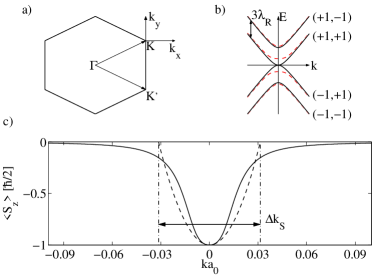
Figure 1: a) Schematic of the hexagonal Brillouin zone of graphene with the $\mathbf{\Gamma}$ point and vectors $\mathbf{K}$, $\mathbf{K}^{\prime}$ pointing to the corresponding corners of the Brillouin zone. The coordinate system that we use in the momentum space is also shown. b) Schematic of the energy bands near the ${K}$ point of the BZ, as obtained from Eq. (3) for $\Delta=0$ (solid) and $\Delta\neq 0$ (dashed). The energy splitting between the spin-split bands is $3\lambda_{R}$ for $\Delta=0$. If $\Delta\neq 0$, a band gap of $\Delta$ opens at $\mathbf{k}=0$. The ($\mu,\nu$) indeces corresponding to a given band are also indicated. c) solid [dashed] line: expectation value of the $z$ component of the spin as a function of $k=|\mathbf{k}|$ (in units of the carbon-carbon bond length $a_{0}$) in the upper valance band ($\mu=-1$, $\nu=1$) calculated from Eq. (7) [Eq. (8)]. The interplay of sublattice asymmetry and RSOI leads to a finite $\langle S_{z}\rangle$. The width of the peak, as defined in the figure, is independent of the asymmetry parameter $\Delta$ [see text below Eq. (8)].

Expanding the right hand side of Eq. (7) assuming that $\hbar v_{F}k\ll\lambda_{R}$ we find for the $\nu=1$ bands:

$${}^{\mu,1}\langle S_{z}\rangle\approx\mu\left(1-\frac{2\hbar^{2}v_{F}^{2}k^{2}}{9\lambda_{R}^{2}}\right)$$ (8)

which one can use to give an estimate of the wavenumber range where the spin $z$ component is non-zero. Fig. 1(c) shows the $z$ polarization computed using Eq. (7) and its approximation from Eq. (8). Estimating the width of the peak by the $k$ values where Eq. (8) becomes zero we find $\Delta k_{S}=3\sqrt{2}\lambda_{R}/\hbar v_{F}$, which is independent of the asymmetry parameter $\Delta$. Taking $v_{F}\approx 10^{6}{\rm m/s}$ and e.g. $\lambda_{R}\approx 20\,{\rm meV}$ we find that $\Delta k_{S}\approx 0.01{\rm\AA^{-1}}$.

III Theoretical description of SARPES for Graphene

In this and the next section we will analyze the effects of sublattice asymmetry on the SARPES spectra performing both analytical and numerical calculations. As in most of the relevant graphene literaturefalko ; kuemmeth ; shirley , we assume that the emitted photoelectrons can be characterized by a simple plane wave of momentum $\mathbf{p}$, spin $\sigma$ and energy $E_{\mathbf{p},\sigma}=\frac{\mathbf{p}^{2}}{2m_{e}}$ (however, see e.g. Ref. s-polar, for the limitations of this assumption). The flux of photoelectrons emitted from an initial state of momentum $\hbar(\mathbf{K}+\mathbf{k})$, energy $\varepsilon_{\mu\nu}(\mathbf{k})$ in band $(\mu,\nu)$ is found to be

$$\begin{split}{}^{\mu,\nu}I\propto&{\rm Tr}\;\bigg{(}\widetilde{Q}^{\mu,\nu}({\bf k})\bigg{)}\;\\ &\delta_{\mathbf{p}_{\parallel}/\hbar-(\mathbf{K}+\mathbf{k}+\mathbf{G}),\mathbf{0}}\;\delta(\hbar\omega+\varepsilon_{\mu\nu}(\mathbf{k})-E_{{\bf p},\sigma}-W)\;.\end{split}$$ (9)

[Some details of the calculations leading to Eq. (9) and Eq. (14) below are given in Appendix A.] Here $\widetilde{Q}^{\mu,\nu}({\bf k})$ is a $2\times 2$ projector onto the photoelectron spinor:

$$\widetilde{Q}_{ij}^{\mu,\nu}({\bf k})=\sum\limits_{k=2i-1}^{2i}\sum\limits_{l=2j-1}^{2j}\left(UQ^{\mu,\nu}({\bf k})U^{\dagger}\right)_{kl},$$ (10)

where $Q^{\mu,\nu}$ was introduced after Eq. (5) and the unitary matrix $U$ is given by

$$U=\left(\begin{smallmatrix}1&0&0&0\\ 0&e^{-{\rm i}{\bf G}{\boldsymbol{\tau}}}&0&0\\ 0&0&1&0\\ 0&0&0&e^{-{\rm i}{\bf G}{\boldsymbol{\tau}}}\end{smallmatrix}\right)\;.$$ (11)

Here $\mathbf{G}$ is an arbitrary reciprocal lattice vector and $\boldsymbol{\tau}$ is a vector pointing from lattice site $B$ to site $A$ in the unit cell of graphene. In the following we will always take ${\bf G}={\bf 0}$, since we will concentrate on one BZ. The Kronecker delta in Eq. (14) expresses momentum conservation ($\mathbf{p}_{\parallel}$ is the component of the momentum of photoelectrons parallel with the graphene surface). Finally, the Dirac delta function in Eq. (14) ensures the energy conservation ($W$ being the work function of graphene). We do not address the question of dynamical processes that lead to energy broadening but use a phenomenological approach by introducing a Lorentzian $\delta(\varepsilon)\rightarrow\frac{\Gamma^{2}}{\varepsilon^{2}+\Gamma^{2}}$ (see Ref. lorentzian, ) in the figures of Section IV with the parameter $\Gamma$ representing the value of the broadening. To keep the formulae uncluttered we suppress henceforth the Kronecker and Dirac delta functions expressing the momentum and energy conservation, they should be understood to appear on the right hand side of Eqs. (12)-(15c) below.

Using the explicit form of the quasiparticle spinors, calculations detailed in Appendix A yield

$${}^{\mu,\nu}I\propto\left(1-\frac{v_{F}\hbar k_{y}(\mathcal{N}(k)-\nu\lambda_{R}^{2})}{\mathcal{N}(k)\varepsilon_{\mu\nu}({\bf k})}\right).$$ (12)

As in previous theoretical worksfalko ; kuemmeth ; shirley (which however did not consider either RSOIshirley ; falko or sublattice asymmetrykuemmeth ) we find a strongly anisotropic photoelectron intensity [see e.g. numerical results in Fig. 2(a)] which originates from sublattice interferencefalko and therefore it is presentintensity-pattern even if $\lambda_{R}=0$. Such anisotropy was observed experimentallyvarykhalov ; giant ; zhou ; bostwick-1 ; bostwick-1 ; sic-gap too. Indeed, Eq. (12) for large wave numbers ($\hbar v_{F}k\gg|\lambda_{R}|$) can be approximated by

$${}^{\mu,\nu}I\propto\left(1-\frac{v_{F}\hbar k_{y}}{\varepsilon_{\mu\nu}({\bf k})}\right)$$ (13)

from where it is easy to see that the intensity is minimal in the region where $k_{y}\gg|k_{x}|,|\Delta|/(\hbar v_{F}),|\lambda_{R}|/(\hbar v_{F})$ and $\mu k_{y}>0$. (By introducing the parametrization $(k_{x},k_{y})=k\,(\sin\theta,\cos\theta)$ one can see that ${}^{\mu,\nu}I$ takes a similar form to the result of Ref. kuemmeth, , though in our notation the indices ${\mu,\nu}$ have slightly different meaning.) Since the intensity of photoelectrons tends to vanish in this region, the authors of Refs. giant, ; kuemmeth, called this region a dark corridor. For $\mathbf{k}\rightarrow 0$, in contrast, the intensity is isotropic. [We note that as the recent experiment of Gierz et al showed [Ref. (s-polar, )], the angular distribution of photoelectron intensity also depends on the energy and polarization of the incident light. Our calculations should be relevant for $p$-polarized incident light.]

In terms of $\widetilde{Q}^{\mu,\nu}$, the expectation value of an operator $\hat{O}$ which gives the result of a measurement on photoelectrons coming from band $(\mu,\nu)$ is given by

$${}^{\mu,\nu}\langle O\rangle({\bf p})=\bigg{.}{\rm Tr}\;\bigg{(}\hat{O}\widetilde{Q}^{\mu,\nu}({\bf k})\bigg{)}\;\bigg{/}\;{\rm Tr}\;\bigg{(}\widetilde{Q}^{\mu,\nu}({\bf k})\bigg{)}.\\$$ (14)

We make use of Eq. (14) to calculate the photoelectron spin-polarization vector $(\mathcal{P}_{x},\mathcal{P}_{y},\mathcal{P}_{z})=\frac{2}{\hbar}(\langle\hat{s}_{x}\rangle,\langle\hat{s}_{y}\rangle,\langle\hat{s}_{z}\rangle)$ where the operator $\hat{s}_{x,y,z}=\sigma_{x,y,z}$ acts on the photoelectron spin. Using Eqs. (14) and (12) we find for the components of the polarization that

$${}^{\mu,\nu}\mathcal{P}_{x}\propto\frac{\nu\lambda_{R}\left(\frac{3}{2}\lambda_{R}^{2}+\frac{2}{3}v_{F}\hbar k_{y}\left(v_{F}\hbar k_{y}-\varepsilon_{\mu\nu}({\bf k})\right)\right)-\frac{3}{2}\lambda_{R}\mathcal{N}(k)}{\mathcal{N}(k)\varepsilon_{\mu\nu}({\bf k})-v_{F}\hbar k_{y}(\mathcal{N}(k)-\nu\lambda_{R}^{2})},$$ (15a)

$${}^{\mu,\nu}\mathcal{P}_{y}\propto\nu\;\frac{\frac{2}{3}v_{F}\hbar k_{x}\;\lambda_{R}\left(\varepsilon_{\mu\nu}({\bf k})-v_{F}\hbar k_{y}\right)}{\mathcal{N}(k)\varepsilon_{\mu\nu}({\bf k})-v_{F}\hbar k_{y}(\mathcal{N}(k)-\nu\lambda_{R}^{2})},$$ (15b)

and

$${}^{\mu,\nu}\mathcal{P}_{z}\propto\nu\;\frac{\frac{1}{2}\Delta\lambda_{R}^{2}}{\mathcal{N}(k)\varepsilon_{\mu\nu}({\bf k})-v_{F}\hbar k_{y}(\mathcal{N}(k)-\nu\lambda_{R}^{2})}.$$ (15c)

It is immediately clear from Eq. (15c) that similarly to Bloch electrons, photoelectrons also acquire a finite $z$ polarization due to the interplay of sublattice asymmetry and RSOI. The magnitude of ${}^{\mu,\nu}\mathcal{P}_{z}$ is largest at the Dirac point for the $\nu=1$ bands where it reaches the value of unity. For the $\nu=-1$ bands the photoelectron polarization is smaller: ${}^{\mu,-1}\mathcal{P}_{z}(k=0)=-\Delta/\sqrt{\Delta^{2}+36\lambda_{R}^{2}}$. In fact, as the density plot in Fig. 2(c) shows for the upper valence band, ${}^{-1,1}\mathcal{P}_{z}(\mathbf{k})$ is finite everywhere in the dark corridor and is very small outside it (the plots for other bands are similar and thus not shown).

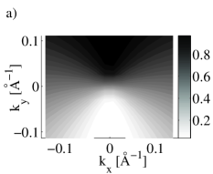
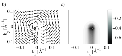
Figure 2: a) intensity distribution; b) and c) spin-polarization of photoelectrons emanating from the upper valance band ($\mu=-1$, $\nu=1$) for momentums close to the ${K}$ point. In b) vector plot of the in-plane component of the spin polarization is shown. In c) density plot of the $z$ component of spin indicates the regions in the BZ where the out-of-plane polarization is finite. We used $\Delta=40\;{\rm meV}$, $\lambda_{R}=66\;{\rm meV}$ in these calculations.

This suggests that in a constant energy SARPES measurement the easiest way to observe the finite $z$ polarization is to use energies close to the Dirac point, otherwise one would have to collect data from the dark corridor, which is difficult due to the low photoelectron intensity and spin-detector efficiency.

Regarding the in-plane component of the photoelectron spin, Ref. kuemmeth, has found that in the case of equivalent sublattices it exhibits a rather peculiar behavior, especially in and close to the dark corridor, where the photoelectron spin is rotated with respect to the quasiparticle spin. Moreover, Ref. kuemmeth, also showed that the in-plane spin polarization of photoelectrons is not zero in the ${K}$ point even though the mean spin of Bloch electrons is zero there [see Eqs. (6)]. We find from Eqs. (15a) and (15b) that the breaking of the $AB$ symmetry does not alter significantly this picture of the in-plane polarization, thus we will only briefly discuss it. An example of the photoelectron in-plane spin polarization is shown in Fig. 2(b) for the upper valence band. One can clearly observe that the spins are rotated in the dark corridor (at $k_{y}<0$, $k_{x}\approx 0$, see Fig. 2(a) where the intensity map is shown for the same band). In contrast to the in-plane spin of quasiparticles, the corresponding spin component of photoelectrons therefore does not show rotational symmetry around the ${K}$ point.

The opening of a small gap at the Dirac point due to the $AB$ symmetry breaking effect of a substrate is not easy to detect in an ARPES measurements because of the finite energy resolution of the experiments and because of the energy broadening of the bands. In the next section we investigate the possibility of detecting the sublattice asymmetry through photoelectron spin polarization. To this end we compute the intensity maps and spin polarization distributions of photoelectrons at given energies.

IV Numerical (S)ARPES calculations

In this section we discuss the results of numerical calculations of constant-energy intensity maps and spin polarizations along certain directions in the BZ. In Ref. sajat, we showed that the Hamiltonian of monolayer graphene for finite RSOI is formally the same as the Hamiltonian of bilayer graphene, if certain weak hopping amplitudes in the latter system can be neglected. The aim of this section is twofold. Firstly, we point out both the similarities and the differences in the constant energy ARPES intensity maps of monolayer graphene with RSOI and bilayer graphene. Secondly, we show photoelectron spin polarization calculations along certain directions in the BZ (spin-resolved MDCs) and relate them to the fixed energy ARPES intensity maps. In the calculation of spin-resolved MDCs we assume that the background is small and disregard its influence on the lineshapessarpes-1 . Since the $AB$ asymmetry does not break the particle-hole symmetry of the Hamiltonian, we only show calculations for energies in the valence bands. We assume strong RSOI and use $\lambda_{R}=66\,{\rm meV}$ corresponding to $\approx 200\,{\rm meV}$ spin-splitting of the bandsgiant .

We start the discussion with intensity maps taken at energies close to the Dirac point. In the derivation of Eq. (12) we neglected those terms in the graphene Hamiltonian which cause trigonal warping of the bands for low energies if RSOI is finite [see the discussion below Eq. (1)]. This approximation is useful to understand the main features of the spin-polarization but for strong RSOI the neglected terms do cause a noticeable change in the fixed-energy intensity maps. In the calculations shown below therefore we take these terms into account as well.

Figure 3: Constant energy (S)ARPES calculations close to the Dirac point. a) and b): schematic band structure at the ${K}$ point of the BZ for zero and finite sublattice asymmetry, respectively. Dashed lines indicate a constant energy cross-section at $E=-37\,{\rm meV}$ where the photoelectron intensity maps in c) and d) are obtained. c) and d): constant energy intensity maps for $\Delta=0$ and $\Delta=40\,{\rm meV}$, respectively. The dashed lines indicate the direction in $\mathbf{k}$ space along which the spin polarization curves in e) and f) are calculated. e) and f): the $x$ (dashed), $y$ (dashed-dotted) and $z$ (solid) component of the photoelectron spin polarization for cross sections shown in c) and d), respectively. (left axis). The dotted lines indicate the intensity profile along the same cross-section (right axis). Subfigures in the left [right] column correspond to sublattice anisotropy parameter $\Delta=0$ [$\Delta=40\;{\rm meV}$]. Other parameters of the figure are $\lambda=66\,{\rm meV}$ and $\Gamma=12.5\,{\rm meV}$.

In Figs. 3(c) and 3(d) only a small broadening of the lines is assumed. Because of the strong RSOI ($\lambda_{R}=66\,{\rm meV}$), small $\Gamma$ and low energy ($E=-37\rm{meV}$) the photoelectrons come predominantly from the upper valence band. One can observe the following important features: similarly to monolayer graphene with zero RSOI (Refs. shirley, ; falko, ) there is a characteristic angular variation in the intensity which is due to sublattice interference and particularly in Fig. 3(c) one can see a low intensity region (the ”dark corridor“) around $k_{x}\approx 0$ and $k_{y}<0$. Nevertheless, as a consequence of spin-pseudospin entanglementkuemmeth at these low energies the intensity distribution is more isotropic in the case of finite RSOI than it is for $\lambda_{R}=0$. Fig. 3(d) shows that the main effect of finite sublattice asymmetry on the intensity maps is that it reduces the intensity anisotropy clearly seen in Fig. 3(c). Comparing e.g. Fig. 3(c) and Fig. 4(c) one can also notice that in the former figure there is a slight trigonal distortion in the intensity contour. This distortion, which is caused by the terms $v_{\lambda}\hat{p}_{\pm}$ in the Hamiltonian (1), can only be seen for strong RSOI and close to the charge neutrality point. Note, that it is different from the trigonal distortion observable for energies far from the Dirac point (see Fig. 6) which is a lattice effect.

Figs. 3(e) and 3(f) show the spin polarization as a function of momentum along the direction indicated by dashed line in Figs.  3(c) and 3(d), respectively. As evidenced by the peaks in the $x$ polarization component $\mathcal{P}_{x}$ [and also noted in Ref. kuemmeth, ], in contrast to Bloch electrons, the spin polarization of photoelectrons is not necesseraly transversal to the momentum $\mathbf{k}$. One can also see that $\mathcal{P}_{y}$ changes sign as the $k_{x}=0$ line is crossed. The out-of-plane component of the photoelectron spin is zero if no sublattice asymmetry is assumed [Fig. 3(f)] but $\mathcal{P}_{z}$ is finite if $\Delta\neq 0$, as in Fig. 3(e). This means that through SARPES measurements in systems where RSOI is nonzero the $AB$ asymmetry can be detected even if the sample is slightly $p$-doped, i.e. states around the Dirac-point are not directly available by ARPES.

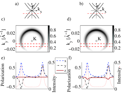
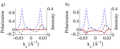
Figure 4: Constant energy (S)ARPES calculations for low energies and small broadening $\Gamma$. a) and b): schematic band structure at the ${K}$ point of the BZ for zero and finite sublattice asymmetry, respectively. Dashed lines indicate a constant energy cross-section at $E=-110\;{\rm meV}$ where the photoelectron intensity maps in c) and d) are obtained. c) and d): constant energy intensity maps for $\Delta=0$ and $\Delta=40\;{\rm meV}$, respectively. The dashed line at $k_{y}=-0.007{\rm\AA^{-1}}$ [$k_{y}=-0.014{\rm\AA^{-1}}$] indicate the direction in $\mathbf{k}$ space along which the spin polarization curves in subfigures e) and f) [ g) and h) ] are calculated. e) and g) [ f) and h) ]: the $x$ (dashed), $y$ (dashed-dotted) and $z$ (solid) component of the photoelectron spin polarization for the two cross sections shown in c) [ d)] (left axis). The dotted lines indicate the intensity profile along the same cross-section (right axis). Subfigures in the left [right] column correspond to sublattice anisotropy parameter $\Delta=0$ [$\Delta=40\;{\rm meV}$]. Other parameters of the figure are $\lambda=66\;{\rm meV}$ and $\Gamma=16.7\;{\rm meV}$.

In Fig. 4 the constant energy maps are calculated at $E=-110\,{\rm meV}$, i.e. not in the close vicinity of the charge neutrality point. As the schematic figures  4(a) and  4(b) show, because of the large spin-splitting (and a small broadening of $\Gamma=16.7\;{\rm meV}$) assumed, all the photoelectrons would still originate from the same band as in the previous case. The intensity maps in Figs. 4(c) and (d) resemble closely the corresponding maps of monolayer graphene (see e.g. Fig. 2 in Ref. falko, ). In particular, one can observe an almost complete suppression of intensity in the dark corridor and the disappearance of the trigonal distortion of the intensity maps, apparent in Figs. 3(c) and (d). Furthermore, comparing Fig. 4(c) and Fig. 4(d) one can see that the presence of a small asymmetry gap [$\Delta=40\,{\rm meV}$ in Fig. 4(d)] would be practically undetectable in an ARPES measurement at this energy. Nevertheless, as Fig. 4(f) and Fig. 4(h) show, if $\Delta\neq 0$ there is a small but finite $z$ polarization component. Comparison of Fig. 4(f) and Fig. 4(h) illustrates the feature shown in Fig. 2(c): $\mathcal{P}_{z}(\mathbf{k})$ is largest in the dark corridor, therefore in a constant energy measurement it is larger if the direction in the $\mathbf{k}$ space is chosen such that it is closer to the dark corridor [ Fig. 4(f) is calculated for $k_{y}=-0.007{\rm\AA^{-1}}$ with maximal polarization of $\mathcal{P}_{z}^{max}=-0.12$, whereas $k_{y}=-0.14{\rm\AA^{-1}}$ in Fig. 4(h) and $\mathcal{P}_{z}^{max}=-0.17$]. Note, that even in the case of Fig. 4(h) the curve is not actually calculated in the dark corridor, the ARPES intensity peaks (shown by dotted line) for this cross-section are roughly $40\%$ of the maximum intensity that can be found at this energy [black arc close to the upper edge of Fig. 4(d)]. On the other hand, the in-plane components of the spin polarization are practically the same for the $\Delta=0$ [Figs. 4(e), 4(g)] and $\Delta\neq 0$ [Figs. 4(f), 4(h)] cases.

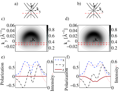
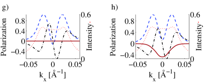
Figure 5: The effects of the broadening parameter $\Gamma$ on the (S)ARPES spectra. As in Fig. 4, all calculations are for $E=-110\,{\rm meV}$. a) and b): the same as in Fig. 4. c) and d): constant energy intensity maps for $\Delta=0$ and $\Delta=40\;{\rm meV}$, respectively. The dashed line at $k_{y}=-0.007{\rm\AA^{-1}}$ [$k_{y}=-0.014{\rm\AA^{-1}}$] indicate the direction in $\mathbf{k}$ space along which the spin polarization curves in subfigures e) and f) [g) and h)] are calculated. e) and g) [ f) and g) ]: the $x$ (dashed), $y$ (dashed-dotted) and $z$ (solid) component of the photoelectron spin polarization for the two cross-sections shown in c) [ d) ] (left axis). The dotted lines indicate the intensity profile along the same cross-section (right axis). Subfigures in the left [right] column correspond to sublattice anisotropy parameter $\Delta=0$ [$\Delta=40\;{\rm meV}$]. Other physical parameters of the figure are $\lambda=66\;{\rm meV}$ and $\Gamma=83.5\;{\rm meV}$.

In ARPES measurements the energy broadening is often quite substantial. To see the effects of broadening on the SARPES spectra we repeated the calculations shown in Fig. 4 for a larger broadening parameter. The results for $\Gamma=83.5\;{\rm meV}$ are presented in Fig. 5. Although the ARPES fixed energy contours are significantly blurred due to the large $\Gamma$, [Figs. 5(c) and 5(d)] the broadening would actually lead to a bigger out-of-plane spin polarization amplitude see Figs. 5(f) and 5(h)], hence it would make the detection of the $z$ spin polarization easier [c.f Figs. 4(f) and 4(h)]. This happens because for large broadening electrons having energies closer to the Dirac point can also contribute and they have larger spin $z$ component. Other noticeable feature in Figs. 5(e)-5(h) compared to Figs. 4(e)-4(h) is that one can clearly see that $\mathcal{P}_{y}$ changes sign three times for small $k_{x}$ values. This is not apparent in e.g. Figs. 4(e) and 4(f) because of the small amplitude of these oscillations there.

Finally, we consider the constant-energy intensity maps and spin polarizations at energy $E=-660\,{\rm meV}$, i.e. quite far from the Dirac point. For these calculations we used the tight-binding Hamiltonian of Ref. kane, . Since this energy is larger than the spin splitting $3\lambda_{R}=200\,{\rm meV}$ used in our calculations, both valence bands contribute to the ARPES and SARPES spectra. We assume for simplicity that the broadening $\Gamma$ is the same for both bands and present calculations with two different $\Gamma$s, the first one being much smaller than the spin-splitting of the bands, while the second one is comparable to it.

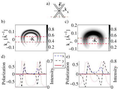
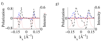
Figure 6: Constant energy (S)ARPES calculations far from the Dirac point. a): schematic band structure at the ${K}$ point. Dashed line indicates a constant energy cross-section at $E=-660\;{\rm meV}$ where the photoelectron intensity maps in b) and c) are obtained. b) and c): constant energy intensity maps for $\Gamma=50\;{\rm meV}$ and $\Gamma=134\;{\rm meV}$, respectively. The dashed lines at $k_{y}=0.035{\rm\AA^{-1}}$ [$k_{y}=-0.035{\rm\AA^{-1}}$] indicate the direction in $\mathbf{k}$ space along which the spin polarization curves in subfigure d) and e) [ f) and g) ] are calculated. d) and f) [e) and g)]: the $x$ (dashed), $y$ (dashed-dotted) and $z$ (solid) component of the photoelectron spin polarization for the two cross sections shown in b) [ c) ] (left axis). The dotted lines indicate the intensity profile along the same cross-section (right axis).

As $E\gg\Delta$ in this case, the ARPES and SARPES spectra are practically the same for $\Delta=0$ or $\Delta\neq 0$, therefore we only show results for $\Delta=0$.

If the broadening is moderate, as in Fig. 6(b), there are two discernible ringlike patterns, each corresponding to photoemission from states in one of the two bands. The rings show slight trigonal distortion, but in contrast to Fig. 3(c), this is a lattice effect and would also be observablefalko for $\lambda_{R}=0$. The double ringlike pattern is reminiscent of the intensity maps found for bilayer graphene at high energiesfalko ; bilayer-arpes , but an important difference is that in Fig. 6(b) both rings have approximately the same intensity. The similarities between the ARPES maps of the two systems are due to the similar bandstructures (for a discussion of the relation between the Hamiltonians of monolayer graphene with RSOI and bilayer graphene see Ref. sajat, ). The difference in the intensity patterns stems from the fact that there are four carbon atoms in the unit cell of bilayer while there are only two in monolayer graphene therefore the transition matrix elements in the photoemission calculations are different.

If the broadening is substantial, as in Fig. 6(c) , the two rings are no longer easily discernible (and they may even completely overlap). Nevertheless, as the dashed-dotted curves in Figs. 6(e) and 6(g) demonstrate, the $y$ component of the spin polarization changes sign as a function of $k_{x}$ roughly in the middle of the intensity peak (dotted line). This is an indication that two bands are involved in the photoemission, as the sign of ${}^{\mu,\nu}\mathcal{P}_{y}$ is different for the $\nu=1$ and $\nu=-1$ bands [see Eq. (15b)]. Furthermore, comparison of Figs. 6(e) and 6(g) [Figs. 6(d) and 6(f)] shows that the overall shape and the number of sign changes in ${}^{\mu,\nu}\mathcal{P}_{y}$ do not depend on whether it is calculated for a positive or negative $k_{y}=const$ value [see Fig. 6(b) or 6(c) for the cross-sections along which Figs. 6(d)-6(g) were obtained]. In contrast, for ${}^{\mu,\nu}\mathcal{P}_{x}$ the number of sign changes in the low intensity region (small $|k_{x}|$ values) is affected by the choice of the $k_{y}$, as e.g the comparison of Figs. 6(e) and 6(g) can illustrate.

V Discussion and Summary

We would first briefly comment on the experimental relevance of our results. As mentioned in the Introduction, a significant spin-orbit coupling was found in gold intercalated Ni(111)/graphene systemvarykhalov and the SOI was attributed to the presence of the gold atoms. Spin-resolved MDCs were not shown however in Ref. varykhalov, . Subsequently, Ref.ruthenium-gap, proved that gold intercalation can decouple graphene from the Ru(0001) surface as well. Another notable recent development is that gold intercalation has also been used for the Si face of SiC substrategierz-gold where the strong covalent bonds between the SiC(0001) and the first graphitic layer were suppressed by this method resulting in a slightly p-doped graphene that was only weakly influenced by the substrate. SARPES measurements were not published in Refs. ruthenium-gap, ; gierz-gold, , though it would be interesting to know if gold can induce SOI in these systems as well. The Ru(0001)/gold/graphene system appears to be particularly interesting from our point of view because ARPES measurement indicate a band gap $>100\,{\rm meV}$, so that if RSOI is non-zero in this system then a finite out-of-plane polarization of photoelectrons should be measurable. A qualitatively similar polarization to the one predicted by this model, with an ”abrupt rotation of the spin“ at the $K$ point of the BZ was measured when thallium was deposited on Si(111) surfacesakamoto , though Ref. sakamoto, explained the effect by the presence of a local effective magnetic field. Finally, we note that Ref. giant, reported a large and anisotropic spin splitting in graphene, including a nonzero out-of plane polarization component, but the origin of this effect seems to be unclear at the moment.

In summary, we studied the effect of RSOI and substrate induced sublattice asymmetry on the spin polarization of quasiparticles and of photoelectrons in graphene. The breaking of $AB$ sublattice symmetry opens a gap in the band structure of graphene at the $K$ point of the BZ. If RSOI is finite, the interplay of the two effects induces a non-zero out-of-plane component of spin polarization of quasiparticles in part of the BZ. RSOI also affects the intensity and spin distribution of photoelectrons, hence it can be studied with the (S)ARPES technique. For strong RSOI, the fixed-energy intensity maps taken at low energies, close to the $K$ point of the BZ, show a characteristic trigonal deformation. This deformation of the intensity map survives the switching-on of an $AB$ symmetry breaking potential given by the asymmetry parameter $\Delta$, as long as $\Delta$ is much smaller than the RSOI induced band splitting. Our spin-resolved MDCs calculations also show that an important sign of the simultaneous presence of RSOI and sublattice asymmetry is if non-zero out-of-plane photoelectron spin polarization can be measured. It is important however, especially if $\Delta$ and RSOI are small, to choose the energy at which the spin-resolved MDCs are taken as close as possible to the Dirac-point, because for energies far from it the out-of-plane polarization remains finite only in the ”dark corridor”, where the low photoelectron intensity would hinder the observation of this effect. A carefully chosen cross-section in the momentum space or a large intrinsic energy broadening may, however, facilitate the observation of the spin $z$ polarization in MDCs even at higher energies. Meanwhile, the in-plane components of photoelectron polarization remain qualitatively the same regardless of whether $\Delta$ is zero or not. If the fixed-energy intensity map is obtained at energies larger than the energy separation of two spin-split bands and their intrinsic energy broadening $\Gamma$ is small compared to their RSOI induced energy splitting, then the resulting ARPES calculation shows a double ring-like structure. For large $\Gamma$, the two rings may not be discernible any more, but SARPES measurements can nevertheless reveal the true band structure because of the sign-changes in the polarization components.

VI Acknowledgments

This work was supported by the Marie Curie ITN project NanoCTM (FP7-PEOPLE-ITN-2008-234970), the Hungarian Science Foundation OTKA under the contracts No. 75529 and No. 81492 and the European Union and the European Social Fund have provided financial support to the project under the grant agreement TÁMOP 4.2.1./B-09/1/KMR-2010-0003. A.K. also acknowledges the support of EPSRC.

Appendix A Outline of the theoretical SARPES calculations

Here we briefly describe the calculation leading to Eq. (14). The Hamiltonian of the interaction between the Bloch electrons and the electromagnetic field in dipole approximationshirley is given by

$$\hat{H}_{int}\propto-\frac{\hbar}{{\rm i}}{\boldsymbol{A}\nabla}\;,$$ (16)

where ${\bf A}={\bf A_{0}}e^{{\rm i}({\bf qr}-\omega t)}$ is the vector potential. The transition probability between an initial Bloch electron state $|{\bf k},(\mu,\nu)\rangle$ and a photoelectron state $|{\bf p},\sigma\rangle$ will be proportional to $|\left(H_{int}\right)_{\textbf{k},(\mu,\nu)}^{\textbf{p},\sigma}|^{2}\,\,\delta(\hbar\omega+\varepsilon_{\mu\nu}(\mathbf{k})-E_{{\bf p},\sigma}-W)$, where the photoexcitation matrix element is

$$\left(H_{int}\right)_{\textbf{k},(\mu,\nu)}^{\textbf{p},\sigma}=\langle{\bf p},\sigma|\hat{H}_{int}|{\bf k},(\mu,\nu)\rangle.$$ (17)

Explicit expression for $\left(H_{int}\right)_{\textbf{k},(\mu,\nu)}^{\textbf{p},\sigma}$ can obtained by assuming that the wavefunction of a photoelectron given by a plane wave $|{\bf p},\sigma\rangle\propto e^{{\rm i}\bf pr/\hbar}|\sigma\rangle$ and the wavefunction of a Bloch electron is

$$\begin{split}|{\bf k},(\mu,\nu)\rangle&=\frac{1}{\sqrt{\mathcal{N}({\bf k})}}\sum\limits_{j=\{A,B\},\sigma^{\prime}=\{\uparrow,\downarrow\}}\Bigg{[}\\ &\psi_{j\sigma^{\prime}}^{\mu\nu}({\bf k})\;|\sigma^{\prime}\rangle\left[\frac{1}{\sqrt{N}}\sum\limits_{n=1}^{N}e^{{\rm i}(\textbf{k+K})\textbf{R}^{j}_{n}}\Phi({\bf r-R}^{j}_{n})\right]\Bigg{]}\;.\end{split}$$ (18)

Here ${\bf R}^{j}_{n}$ are vectors pointing to sublattice sites $j=\{A,B\}$ in unit cell $n$, $N$ is the number of unit cells in the sample, $\psi_{j\sigma^{\prime}}^{\mu\nu}({\bf k})$ are the amplitudes of Bloch electrons on sublattice $j$ with momentum ${\bf k}$ and spin $\sigma^{\prime}$ and finally, $\Phi(\mathbf{r})$ is a $p_{z}$ atomic orbital. The photoexcitation matrix element then reads:

$$\left(H_{int}\right)_{\textbf{k},(\mu,\nu)}^{\textbf{p},\sigma}\propto\sqrt{N}\Phi_{p}({\bf Ap})\bigg{(}\psi_{A\sigma}^{\mu}({\bf k})+e^{{\rm i}{\bf G}{\boldsymbol{\tau}}}\psi_{B\sigma}^{\mu}({\bf k})\bigg{)}.$$ (19)

In Eq. (19) $\Phi_{\mathbf{p}}$ is the Fourier transform of the atomic orbital $\Phi(\mathbf{r})$, and ${\bf G}=m_{1}{\bf b_{1}}+m_{2}{\bf b_{2}}$ is a reciprocal lattice vector which is given in terms of primitive lattice vectors $\mathbf{b}_{1}=(2\pi/a_{0},2\pi/\sqrt{3}\,a_{0})$, $\mathbf{b}_{2}=(2\pi/a_{0},-2\pi/\sqrt{3}\,a_{0})$ and integers $m_{1}$, $m_{2}$. Furthermore, ${\boldsymbol{\tau}}\equiv{\bf R^{B}_{n}-R^{A}_{n}}$ and ${\bf p}_{\parallel}$ is the projection of momentum $\bf p$ onto the plane of graphene. By defining

$$|\Phi_{\bf p}^{(\mu,\nu)}\rangle=\sum_{\sigma=\{\uparrow,\downarrow\}}\left(H_{int}\right)_{\textbf{k},(\mu,\nu)}^{\textbf{p},\sigma}|{\bf p},\sigma\rangle,$$ (20)

the expectation value of an operator $\hat{O}$ with respect to the photoelectron state emanating from an initial Bloch state of momentum $\hbar(\mathbf{K}+\mathbf{k})$, energy $\varepsilon_{\mu\nu}(\mathbf{k})$ in band $(\mu,\nu)$ can be calculated as

$$\begin{split}{}^{\mu,\nu}\langle O\rangle({\bf p})=&\frac{\langle\Phi_{\bf p}^{(\mu,\nu)}|\hat{O}|\Phi_{\bf p}^{(\mu,\nu)}\rangle}{\langle\Phi_{\bf p}^{(\mu,\nu)}|\Phi_{\bf p}^{(\mu,\nu)}\rangle}\times\\ &\delta_{\bf p_{\parallel}/\hbar-(K+k+G),0}\,\delta(\hbar\omega+\varepsilon_{\mu\nu}(\mathbf{k})-E_{{\bf p},\sigma}-W).\end{split}$$ (21)

Eq. (14) then follows from Eqs. (19) and (21). We note that a convenient way of calculating the projectors $Q^{\mu,\nu}({\bf k})$ which are necessary to evaluate Eqs. (9) and (14) [see Eq. (10)] is to make use of the following: if one denotes by $E_{j}$, $j=1\dots n_{d}$, $n_{d}\leq N$ the distinct eigenvalues of a $N\times N$ hermitian matrix $H$, then the projector onto the $\eta$th eigenstate is given by the expression

$$Q^{\eta}=\frac{\prod\limits_{\eta\neq j}\left(H-E_{j}\hat{I}\right)}{\prod\limits_{\eta\neq j}\left(E_{\eta}-E_{j}\right)}\;,$$ (22)

which does not necessitates the calculation of the eigenvectors. In the mathematical literature the projectors $Q^{\eta}$ are known as Frobenius covariantsfrob-cov . In terms of the projectors $Q^{j}$ and eigenvalues $E_{j}$ the matrix $H$ is given by $H=\sum_{j=1}^{n_{d}}E_{j}Q^{j}$.

References

- (1) A. K. Geim and K. S. Novoselov, Nature Mater. 6, 183 (2007).
- (2) N. Tombros, Cs. Jozsa, M. Popinciuc, H. T. Jonkman and B. J. van Wees, Nature 448, 571 (2007).
- (3) A. Varykhalov, J. Sánchez-Barriga, A. M. Shikin, C. Biswas, E. Vescovo, A. Rybkin, D. Marchenko, and O. Rader, Phys. Rev. Lett. 101, 157601 (2008).
- (4) I. Gierz, J. H. Dil, F. Meier, B. Slomski, J. Osterwalder, J. Henk, R. Winkler, C. R. Ast, K. Kern, arXiv:1004.1573v2 (unpublished).
- (5) C. L. Kane and E. J. Mele, Phys. Rev. Lett. 95, 226801 (2005).
- (6) D. Huertas-Hernando, F. Guinea, and A. Brataas, Phys. Rev. B 74, 155426 (2006).
- (7) H. Min, J. E. Hill, N. A. Sinitsyn, B. R. Sahu, L. Kleinman, and A. H. MacDonald, Phys. Rev. B 74, 165310 (2006) Y. Yao, F. Ye, X.-L. Qi, S.-C. Zhang, and Z. Fang, ibid. 75, 041401 (2007); J. C. Boettger, and S. B. Trickey, ibid. 75, 121402 (2007).
- (8) M. Gmitra, S. Konschuh, C. Ertler, C. Ambrosch-Draxl, and J. Fabian, Phys. Rev. B 80, 235431 (2009); S. Konschuh, M. Gmitra, and J. Fabian, Phys. Rev. B 82, 245412 (2010).
- (9) S. Abdelouahed, A. Ernst, J. Henk, I. V. Maznichenko, and I. Mertig, Phys. Rev. B 82, 125424 (2010).
- (10) E. I. Rashba, Phys. Rev. B 79, 161409 (2009).
- (11) M. H. Kang, S. Ch. Jung, and J. W. Park, Phys. Rev. B 82, 085409 (2010).
- (12) C, Enderlein, Y. S. Kim, A. Bostwick, E. Rotenberg, and K. Horn, New Journal of Physics 12, 033014 (2010).
- (13) A. Grüneis and D. V. Vyalikh, Phys. Rev. B 77, 193401 (2010).
- (14) J. Wintterlin and M. L. Bocquet, Surface Science 603, 1841 (2009).
- (15) Seungchul Kim, Jisoon Ihm, Hyoung Joon Choi, and Young-Woo Son, Phys. Rev. Lett. 100, 176802 (2008).
- (16) Y. Qi, S. H. Rhim, G. F. Sun, M. Weinert, and L. Li, Phys. Rev. Lett. 105, 085502 (2010).
- (17) O. Pankratov, S. Hensel, and M. Bockstedte, Phys. Rev. B 82, 121416(R) (2010).
- (18) I. Gierz, T. Suzuki, R. Th. Weitz, D. S. Lee, B. Krauss, Ch. Riedl, U. Starke, H. Höchst, J. H. Smet, Ch. R. Ast, and K. Kern, Phys. Rev. B 81, 235408 (2010).
- (19) C. Riedl, C. Coletti, T. Iwasaki, A. A. Zakharov, and U. Starke, Phys. Rev. Lett. 103, 246804 (2009).
- (20) D. A. Siegel, C. G. Hwang, A. V. Fedorov, and A. Lanzara, Phys. Rev. B 81, 241417(R) (2010).
- (21) U. Starke and C. Riedl, J. Phys.:Condens. Matter 21, 134016 (2009).
- (22) A. Damascelli, Z. Hussain, and Zhi-Xun Shen, Rev. Mod. Phys. 75, 473 (2003).
- (23) J. Braun, Rep. Prog. Phys. 59, 1267 (1996).
- (24) S. Y. Zhou, G.-H. Gweon, J. Graf, A. V. Fedorov, C. D. Spataru, R. D. Diehl, Y. Kopelevich, D.-H. Lee, S. G. Louie, and A. Lanzara, Nat. Phys. 2, 595 (2006).
- (25) A. Bostwick, T. Ohta, T. Seyller, K. Horn, and E. Rotenberg, Nat. Phys. 3, 36 (2007).
- (26) A. Bostwick, T. Ohta, J. McChesney, K. V. Emtsev, T. Seyller, K. Horn, and E. Rotenberg, New J. Phys. 9, 385 (2007).
- (27) I. Pletikosić, M. Kralj, P. Pervan, R. Brako, J. Coraux, A. T. N’Diaye, C. Busse, and T. Michely, Phys. Rev. Lett. 102, 056808 (2009).
- (28) M. Sprinkle, D. Siegel, Y. Hu, J. Hicks, A. Tejeda, A. Taleb-Ibrahimi, P. Le Févre, F. Bertran, S. Vizzini, H. Enriquez, S. Chiang, P. Soukiassian, C. Berger, W. A. de Heer, A. Lanzara, and E. H. Conrad, Phys. Rev. Lett. 103, 226803 (2009).
- (29) S. Y. Zhou, G.-H. Gweon, A. V. Fedorov, P. N. First, W. A. de Heer, D.-H. Lee, F. Guinea, A. H. Castro Neto and A. Lanzara, Nature Materials 6, 770 (2007).
- (30) I. Gierz, J. Henk, H. Höchst, Ch. R. Ast, and K. Kern, arXiv:1010.1618 (unpublished).
- (31) J. Hugo Dil, J. Phys.:Condens. Matter 21, 403001 (2009).
- (32) F. Meier, J. H. Dil, and J. Osterwalder, New Journal of Physics 11, 125008 (2009).
- (33) M. Mucha-Kruczyński, O. Tsyplyatyev, A. Grishin, E. McCann, V. I. Fal’ko, A. Bostwick, and E. Rotenberg, Phys. Rev. B 77, 195403 (2008).
- (34) F. Kuemmeth, and E. I. Rashba, Phys. Rev. B 80, 241409(R) (2009).
- (35) Fig.1(d) of Ref. falko, shows for the intensity pattern at a fixed energy covering several Brilloiun zones. A constant energy cross-section of the calculations shown in Fig. 2(a) at energies away from the Dirac point (so that for this energy ) would give a very similar result to the one in Fig.1(d) of Ref. falko, . Note however, that because of the different choice of the coordinate system, our () corresponds to () in Ref. falko, .
- (36) P. Rakyta, A. Kormányos, and J. Cserti, Phys. Rev. B 82, 113405 (2010).
- (37) Ming-Hao Liu and Ching-Ray Chang, Phys. Rev. B 80, 241304(R) (2010).
- (38) E. L. Shirley, L. J. Terminello, A. Santoni, and F. J. Himpsel, Phys. Rev. B 51, 13614 (1995).
- (39) In Ref. falko a slightly different broadening function was considered: . We found that our choice is more convenient for the spin polarization calculations, the full width at half maximum of the functions, which is of importance here, is the same for both choices.
- (40) T. Ohta, A. Bostwick, Th. Seyller, K. Horn, and E. Rotenberg, Science 313, 951 (2006).
- (41) K. Sakamoto, T. Oda, A. Kimura, K. Miyamoto, M. Tsujikawa, A. Imai1, N. Ueno, H. Namatame, M. Taniguchi, P. E. J. Eriksson, and R. I. G. Uhrberg, Phys. Rev. Lett 102, 096805 (2009).
- (42) R. A. Horn et al., Topics in Matrix Analysis, Cambridge University Press, Cambridge, UK, 1991.