High Performance Gravitational $N$-body Simulations on a Planet-wide Distributed Supercomputer

Abstract

We report on the performance of our cold-dark matter cosmological $N$-body simulation which was carried out concurrently using supercomputers across the globe. We ran simulations on 60 to 750 cores distributed over a variety of supercomputers in Amsterdam (the Netherlands, Europe), in Tokyo (Japan, Asia), Edinburgh (UK, Europe) and Espoo (Finland, Europe). Regardless the network latency of 0.32 seconds and the communication over 30.000 km of optical network cable we are able to achieve $\sim 87$% of the performance compared to an equal number of cores on a single supercomputer. We argue that using widely distributed supercomputers in order to acquire more compute power is technically feasible, and that the largest obstacle is introduced by local scheduling and reservation policies.

1 Introduction

Some applications for large scale simulations require a large amount of compute power. This is often hard to acquire on a single machine. Combining multiple supercomputers to do one large calculation can lift this limitation, but such wide area computing is only suitable for certain algorithms. And even then the political issues, like arranging the network, acquiring the compute time, making reservations, scheduling runtime and synchronizing the run start, and technical limitations are profound. Earlier attempts based on interconnecting PC clusters were quite successful inteugrid ; Gualandris2007 ; Manos ; Bal20083 ; QCGEscience2009 , but lacked the raw supercomputer performance required for our application.

Running simulations across multiple supercomputers has been done a few times before IWay ; paragon ; arthropod ; CosmoGrid , though the performance of simulations across three or more supercomputers has not yet been measured in detail. Here we report on the performance of our parallel astronomical simulations which use up to 4 supercomputers and predict the performance for simulations which use 5 or more supercomputers.

In our experiments we use an international infrastructure of supercomputers. These machines include an IBM Power6 supercomputer located at SARA in Amsterdam (the Netherlands) and three Cray XT-4 supercomputers located at the Edinburgh Parallel Computing Centre in Edinburgh (United Kingdom), the IT Center for Science in Espoo (Finland) and the Center For Computational Astrophysics in Tokyo (Japan). The Edinburgh site is equipped with a 1 Gbps interface while the other three sites are equipped with a 10 Gbps interface. We achieved a peak performance of 0.610 TFLOP/s and a sustained performance of 0.375 TFLOP/s using 120 cores distributed over 4 sites. To provide a comparison with the international tests we also run the code over up to 5 sites on a Dutch grid of PC clusters. Our wide area simulations are realized with the development of a software environment for Simulating the Universe Structure formation on Heterogeneous Infrastructures, or SUSHI for short.

2 Overview of SUSHI

Our code is based on the GreeM cosmological $N$-body integrator, which was originally developed for special-purpose GRAPE hardware 2005PASJ…57..849Y . The code integrates the equations of motion for dark matter particles using a shared and adaptive time step scheme and a Tree/Particle-Mesh (TreePM) force calculation method 1995ApJS…98..355X which assumes periodic boundary conditions. The short range force interactions are resolved using a Barnes-Hut tree algorithm 1986Natur.324..446B while the long range interactions are resolved using a Particle Mesh (PM) algorithm 1981csup.book…..H .

The tree integration method places particles in a three-dimensional sparse octree structure, where each cell contains the center of mass and the mass aggregate of the particles therein. The method then resolves long range force interactions using particles and tree cells instead of using direct particle-particle evaluation. The accuracy of the tree integration method can be tuned by changing the opening angle ($\theta$), which determines how small and distant a group of particles needs to be to use the approximate particle-tree cell evaluation. A higher value for $\theta$ results in fewer particle-particle evaluations, and a lower accuracy of the simulation. Particle integration using a tree algorithm is more compute-intensive than integration using a PM algorithm, but we speed up the calculations by a factor $\sim 8$ using vector-math code optimizations for both the x86 2006NewA…12..169N and Power6 architectures. The PM algorithm maps the particles to a grid of mesh cells and calculates the gravitational potential using the FFTW Fast Fourier Transform fftw . It accurately calculates the forces of long distance interactions, but is less accurate in computing forces over short distances, for which the tree algorithm is applied instead.

The code has been modified to allow simulations on massively parallel machines Ishiyama09 , in which the code uses a recursive multi-section scheme 2004PASJ…56..521M to divide the workload over the processes. The workload is redistributed during each step of the simulation so that the force calculation time remains equal for all processes.

2.1 Parallelization across supercomputers

We have developed SUSHI to efficiently use multiple supercomputers for our simulations. We coupled the TreePM code with the MPWide communication library MPWide and developed a cross-supercomputer parallelization scheme. Because the wide area network has performance and topological characteristics that are different from local networks, the communication scheme between sites is different from the scheme used between nodes. When SUSHI is deployed across sites, each site is connected to two neighboring sites to form a ring topology.

2.1.1 Communication scheme.

A simulation using SUSHI consists of four communication phases per step. During these phases the simulation:

1. Exchanges mesh densities.

2. Collects sample particles to determine the site boundaries,

3. Exchanges tree structures with neighboring sites.

4. Migrates particles between neighboring sites.

When exchanging mesh densities, the mesh cells from all sites are aggregated to obtain the global mesh density. This mesh density is then used to perform PM integration. In the code we have used here the PM integration is still a serial operation, though the time spent on PM integration in our experiments is only a small fraction of the total runtime. However, to support larger meshes efficiently we will introduce parallelized PM integration in a later version of the code. The mesh densities are gathered using a ring communication over all sites. The force calculation time and time step information of each site are also accumulated during this phase.

At each step the site boundaries are updated, based on the obtained force calculation times and the current particle distribution. To gain information on the particle distribution, the communication processes on each site gather sample particles from all other processes. These sampled particles are then gathered from all sites using a ring communication.

Before the tree force calculations can be performed, each site constructs a local essential tree structure. This local essential tree is a set of particles and tree cells which are used to compute the force exchanges, and partially resides on neighboring sites. To obtain a complete local essential tree, each site therefore requires the missing tree data from its neighbors. The simulation gathers the tree data using one neighbor exchange for two site runs, or two exchanges for runs across three or more sites.

After the force calculations have been performed, the simulation updates the positions of all particles. At this point, some particles may be located outside the site boundaries and need to be migrated to a neighboring site. This communication requires one neighbor exchange for two site runs, or two exchanges for runs across three or more sites.

2.1.2 Domain decomposition.

We have implemented a hierarchical decomposition scheme to distribute the particles among supercomputers. This scheme uses a one-dimensional slab decomposition to distribute the particles among the sites, and a recursive multi-section scheme over three dimensions to distribute the particles among the processes. Because the domain decomposition between sites is one-dimensional, each supercomputer only exchanges particles and tree structures with two other machines. The data exchanges between sites can therefore be done efficiently in a ring topology. Most supercomputers are connected by optical paths in either a ring or star topology, if they are connected at all.

The simulation adjusts the distribution of particles among supercomputers at run-time, such that the force calculation time is kept equal on all sites. The number of particles $N_{i}$ on a single site $i$ for a run performed over $s$ sites is therefore given by

$$N_{i}\sim\frac{N\left(t_{\rm calc,i}\right)^{-1}}{\sum_{i=0}^{i<s}\left(t_{\rm calc,i}\right)^{-1}}.$$ (1)

The force calculation time on site $i$ during the previous step is given by $t_{\rm calc,i}$. The load balancing algorithm can be suppressed by explicitly limiting the boundary moving length per step.

2.1.3 Implementation of communication routines.

We use the MPWide communication library MPWide to perform wide area message passing within SUSHI. The implementation of the communication routines has few external dependencies, which makes it easy to install on different platforms. The wide area communications in MPWide are performed using parallel TCP streams. In cases where the supercomputers can only be indirectly connected, we use MPWide-based port forwarding programs on the intermediate nodes to establish a communication path. During the development of SUSHI, we found that it is not trivial to obtain optimal communication performance between supercomputers. Therefore we added several features that can be used to improve the communication performance. The communication routines within SUSHI can be customized for individual paths between supercomputers. Settings that can be adjusted for each connection include the number of parallel TCP streams, the TCP buffer sizes and the size of data packages that are written to or read from the sockets. To improve the performance on some long distance networks, MPWide also supports software-based packet pacing.

2.1.4 Memory consumption.

Simulations run using SUSHI require 60 bytes of memory per particle and 52 bytes per tree node. As we use an $N_{\rm leaf}$ value of 10 (where $N_{\rm leaf}$ is the number of particles where the interaction tree will not be divided further), we have on average 0.75 tree nodes per particle, and therefore require a total of 99 bytes of memory per integrated particle (see Ishiyama09 for further details). Consequently, a simulation with $N=2048^{3}$ requires 850 GB of RAM for tree integration while a run with $N=8192^{3}$ requires at least 54 TB of RAM. In addition, 4.5 bytes per mesh cell is required to do PM integration. These memory constraints place a lower limit on the number of processes that can be used, and indirectly determine the memory required on communication nodes. For particularly large exchange volumes, the code can conserve memory on the communication nodes by communicating in multiple steps.

3 Performance model

We have developed a performance model for SUSHI. The model can be applied to predict the execution time and scalability of simulations that run across supercomputers. To make an accurate prediction we require several architecture-dependent parameters. These include machine-specific parameters such as the time spent on a single tree interaction (given by $\tau_{\rm tree}$), the time required for one FFT operation $\tau_{\rm fft}$ and the time required for the mesh operations on a single particle ($\tau_{\rm mesh}$). In addition, we need a few parameters for the networks used in the simulation, which are the round-trip time (given by $\lambda_{\rm lan}$ and $\lambda_{\rm wan}$) and the available bandwidth ($\sigma_{\rm lan}$ and $\sigma_{\rm wan}$). The values of these parameters can be obtained through minor network tests and a small single process test simulation on each site. The values used for our experiments are found in Tab. 5 for each supercomputer, in Tab. 2 for each national grid site and in Tab. 6 for the local and wide area networks.

3.1 Single supercomputer

The time required for one TreePM integration step using $p$ processes on a single supercomputer ($t_{\rm exec}(1,p)$) consists of time spent on tree force calculations ($t_{\rm tree}$), time spent on PM integration ($t_{\rm pm}$) and the communication overhead ($t_{\rm comm}$):

$$t_{\rm exec}\left(1,p\right) = t_{\rm tree}+t_{\rm pm}+t_{\rm comm}.$$ (2)

The time spent on tree integration ($t_{\rm tree}$) is dominated by force calculations. The force calculation time is obtained by multiplying the time required to perform a single force interaction ($\tau_{\rm tree}$) with the total number of tree interactions ($n_{\rm int}$) and dividing it by the number of processes ($p$). Creating interaction lists and constructing the tree introduce additional overhead that scales with the number of interactions. To account for this in a simplified way, we multiply the time spent on force calculations with a factor 1.2 . The time spent on tree integration then becomes

$$t_{\rm tree} = 1.2\frac{\tau_{\rm tree}n_{\rm int}}{p}.$$ (3)

The number of interactions per simulation step depends on many parameters including, but not limited to, the number of particles ($N$), the opening angle of the tree integration ($\theta$) and the number of mesh cells ($M$). We have performed several runs over a single supercomputer and fitted the number of interactions for cosmological datasets, which results in

$$n_{\rm int}=\frac{460N^{1.0667}}{\theta^{1.35}}\frac{N^{1/12}}{M^{1/12}\sqrt{2.0}}.$$ (4)

In general, $n_{\rm int}\propto\theta^{-1.35}$ although this estimate may not be accurate if $\theta\ {\raise-2.15277pt\hbox{$\buildrel<\over{\sim}$}}\ 0.2$ or $\theta\ {\raise-2.15277pt\hbox{$\buildrel>\over{\sim}$}}\ 0.75$. In these regimes, the number of interactions depends more strongly on other tree integration settings, such as the maximum number of particles allowed to share interaction lists.

We calculate the time spent on PM integration ($t_{\rm pm}$) by adding the time spent on the Fast Fourier Transform (FFT) to the time spent on mesh operations such as interpolating the mesh values and setting the mesh forces on each particle. The FFT requires $O(M\log_{2}M)$) FFT operations fftw , each of which requires ($\tau_{\rm fft}$) seconds. The time required for mesh operations scales with the local number of particles ($N/p$), where the time required per particle is equal to the machine-specific constant $\tau_{\rm mesh}$. The total time spent on PM integration then becomes

$$t_{\rm pm} = \tau_{\rm fft}M\log_{2}M+\tau_{\rm mesh}\frac{N}{p}.$$ (5)

We decompose the communication time ($t_{\rm comm}$) into time spent to initially traverse the networks ($t_{\rm l}$), which is latency-bound and time spent on data throughput ($t_{\rm b}$), which is limited by the available bandwidth of the local network. Therefore,

$$t_{\rm comm} = t_{\rm l}+t_{\rm b}.$$ (6)

For each step, the code performs 18 collective operations containing $\log p$ communication steps and two all-to-all communications with $p$ communication steps. The time spent in latency ($t_{\rm l}$) is calculated by multiplying the number of communication steps with the network round-trip time ($\lambda_{\rm lan}$). As a result,

$$t_{\rm l} = \lambda_{\rm lan}\left(18\log p+2p\right),$$ (7)

We determine the time spent on data throughput ($t_{\rm b}$) by dividing the data volume of the local area communications by the network bandwidth ($\sigma_{\rm lan}$). The communication data volume consists of three dominant parts. These are the mesh cells residing at other processes (which is at most $4M$ bytes in total), the local essential tree structures (estimated to be $\left(48/\theta+24\right)N^{2/3}p^{-2/3}$ bytes for $0.2\ {\raise-2.15277pt\hbox{$\buildrel<\over{\sim}$}}\ \theta\ {\raise-2.15277pt\hbox{$\buildrel<\over{\sim}$}}\ 0.75$), and the sample particles which are used to determine the node boundaries ($12Nr_{\rm samp}$ bytes in total). Here, $r_{\rm samp}$, which we set to $1/10000$ for large calculations, is the ratio of sampled particles relative to $N$. The time spent on data throughput is then

$$t_{\rm b} = \frac{4M+\left(144/\theta+72\right)N^{2/3}p^{-2/3}+12Nr_{\rm samp}}{\sigma_{\rm lan}}.$$ (8)

Additional communication is required to migrate particles between sites. The data volume of this communication is relatively large during initial simulation steps, but becomes negligible once sufficient steps have been taken to adequately balance the workload. A detailed review of the communication characteristics of the code is presented in Ishiyama09 .

3.2 Multiple supercomputers

We calculate the wall-clock time required for a single TreePM integration step using $p$ processes in total across $s$ supercomputers ($t_{\rm exec}(s,p)$) by adding the wide area communication overhead $w_{\rm comm}$ to the time spent on tree integrations ($t_{\rm tree}$), the time spent on PM integration ($t_{\rm pm}$) and the time spent local area communications ($t_{\rm comm}$). The execution time per step is therefore

$$t_{\rm exec}\left(s,p\right) = t_{\rm tree}+t_{\rm pm}+t_{\rm comm}+w_{\rm comm}.$$ (9)

Here, we calculate $t_{\rm tree}$ using Eq. 3, $t_{\rm pm}$ using Eq. 5 and $t_{\rm comm}$ using Eq. 6. Note that for runs across sites we calculate the local latency-bound communication time $t_{\rm l}$ using the number of local processes $p/s$, rather than $p$. The communication overhead on the wide area network ($w_{\rm comm}$) consists of the time spent in latency ($w_{\rm l}$) and the time spent on data throughput ($w_{\rm b}$) on the wide area network. As a result,

$$w_{\rm comm} = w_{\rm l}+w_{\rm b}.$$ (10)

The code performs five blocking gather operations over all sites per step. These gathers are performed using a ring scheme, which requires $s-1$ neighbor exchanges per gather. We also require four blocking exchanges with each of the two neighboring sites. The total number of exchanges is then equal to $5s+3$ and, the total time spent in latency ($w_{\rm l}$) then becomes

$$w_{\rm l} = \lambda_{\rm wan}\left(5s+3\right).$$ (11)

Here, $\lambda_{\rm wan}$ is the network round-trip time between sites.

We calculate the time spent on wide area data throughput ($w_{\rm b}$) by dividing the data volume of the wide area communications by the bandwidth capacity of the wide area network ($\sigma_{\rm wan}$). The volume of the exchanged data between sites is similar to the data volume between nodes with three exceptions. First, the exchange of mesh densities requires one float per mesh cell per site. Second, because SUSHI uses a 1D decomposition between sites the volume of the local essential tree is larger. Third, because of the 1D decomposition we exchange only the Cartesian x coordinates of sampled particles. The data volume for the exchange of sampled particles is therefore three times smaller. The total time spent on wide area data throughput is

$$w_{\rm b} = \frac{4sM+\left(48/\theta+24\right)N^{2/3}+4Nr_{\rm samp}}{\sigma_{\rm wan}}.$$ (12)

3.3 Scalability across sites

The speedup of a simulation across sites, $S\left(s\right)$, is defined by dividing the time required for an integration step on 1 site using $p$ processes ($t_{\rm exec}\left(1,p\right)$) by the time required for an integration step over $s$ sites using a total of $s\cdot p$ processes ($t_{\rm exec}\left(s,sp\right)$). It is therefore given by

$$S\left(s\right)=\frac{t_{\rm exec}\left(1,p\right)}{t_{\rm exec}\left(s,sp\right)}.$$ (13)

The efficiency of a simulation across sites, $E\left(s\right)$, is calculated by dividing the time required for an integration step on 1 site using $p$ processes by the time required for an integration step over $s$ sites using a total of $p$ processes ($t_{\rm exec}\left(s,p\right)$). The efficiency is then

$$E\left(s\right)=\frac{t_{\rm exec}\left(1,p\right)}{t_{\rm exec}\left(s,p\right)}.$$ (14)

4 Experiments

We have tested SUSHI for performance on a grid of 5 Beowulf clusters, as well as an infrastructure consisting of four supercomputers. Each simulation lasts for 100 integration steps, and uses an opening angle of $\theta=0.3$ when the redshift $z>10$ and $\theta=0.5$ when $z\leq 10$. Here the redshift $z$ is used as an indication of time, with the Big Bang occuring at $z=\infty$ and $z=0$ being the present day. For each opening angle we measured the total wall-clock time and communication time per step, averaged over 10 steps. All measurements were made near $z=10$, approximately 460 million years after the Big Bang. A full listing of the simulation parameters and initial condition characteristics of our experiments is given in Tab. 1.

Parameter	Value
Matter density parameter ($\omega_{0}$)	0.3
Cosmological constant ($\lambda_{0}$)	0.7
Hubble constant ($H_{0}$)	70.0 km/s/Mpc
Box size	$(30Mpc)^{3}$
Mass fluctuation parameter ($\sigma_{8}$)	0.9
Softening for $N=256^{3}$/$512^{3}$/$1024^{3}$ run	5/2.5/1.25 Kpc
Sampling rate $r_{\rm samp}$ for $N=256^{3}$	2500
Sampling rate $r_{\rm samp}$ for $N>256^{3}$	10000
Tree opening angle ($\theta$), $z>10$	0.3
Tree opening angle ($\theta$), $z\leq 10$	0.5
Tree ncrit	1000

Table 1: Initial condition and accuracy parameters used for our test simulations. The maximum number of particles allowed to share an interactions list in the tree integration is given by ncrit.

We compare the results of our experiments with predictions from our performance model. To do so, we measured the value of several machine constants using local tests and provide them in Tab. 2 and Tab. 5. The network constants used in the performance model are given in Tab. 6. As all simulations lasted for 100 integration steps, particle exchanges were still performed to improve the distribution of work. We have added the measured average data volume of these exchanges to the data volume for wide area communications in our model. For full-length simulations, the data volume of these particle exchanges becomes a negligible part of the total communication volume.

4.1 DAS-3 experiment setup

The Distributed ASCI Supercomputer 3 (DAS-3 DAS3 ) is a Dutch infrastructure that consists of 5 PC clusters within The Netherlands. The clusters use 10 Gbps networking internally, while the head nodes of each site are connected to regular internet in a star topology. Using end-to-end message passing tests we were able to achieve a performance of up to 1.25 Gbps between sites. The specifications of the five DAS-3 sites can found in Tab. 2.

Site	VU	UvA	LIACS	TU	MM
City	A’dam	A’dam	Leiden	Delft	A’dam
AMD CPU model	DP280	DP275	DP252	DP250	DP250
Number of nodes	85	41	32	68	46
Cores per node	4	4	2	2	2
CPU freq. [GHz]	2.4	2.2	2.6	2.4	2.4
Memory / core [GB]	1	1	2	2	2
Peak [TFLOP/s]	3.26	1.44	0.66	1.31	0.88
$\tau_{\rm tree}$ [$\times 10^{-9}$ s]	5.9	6.4	5.4	5.9	5.9
$\tau_{\rm fft}$ [$\times 10^{-9}$ s]	5.0	5.0	5.7	5.0	5.0
$\tau_{\rm mesh}$ [$\times 10^{-6}$ s]	2.4	2.4	2.4	1.9	2.4
Ordering	$1^{st}$	$2^{nd}$	$3^{rd}$	$4^{th}$	$5^{th}$

Table 2: Technical specifications of five sites of the DAS-3 Dutch Grid. Three of the five DAS-3 sites reside in Amsterdam.

We performed experiments using three problem sizes and two opening angles. For our tests, we performed one set of runs with $N=256^{3}$ particles and $M=128^{3}$ mesh cells using 60 processes distributed evenly among the sites and two sets of runs with $N=512^{3}$ particles using 120 processes in total. One of the runs with $N=512^{3}$ uses $M=128^{3}$ and the other uses $M=256^{3}$. We maintained a fixed site ordering for all our runs as given in the bottom row of Tab. 2. For all our experiments on the DAS-3, we have configured MPWide to use a single TCP stream per communication channel, send messages in chunks of 8 kB and receive messages in chunks of 32 kB. We did not use software-based packet pacing during these tests.

4.2 DAS-3 results

The timing measurements of our experiments can be found respectively in the left panel of Fig. 1 and 2 for the runs with $N=256^{3}$ and in Fig. 3 and 4 for the runs with $N=512^{3}$. Here we see that the total communication overhead (including both local and wide area communications) becomes marginally higher as we increase in number of sites in the simulation with $N=256^{3}$ and $M=128^{3}$ mesh cells, both for runs with $\theta=0.3$ and with $\theta=0.5$. The measured total communication overhead for simulations with $N=512^{3}$ increases more steeply with $s$, because the larger communication data volume results in a higher traffic load on the internet lines between the sites. On the other hand, the time spent on local communications becomes lower when we run SUSHI across more sites. The number of processes per site ($p/s$) is lower for runs across more sites, which results in a smaller load and less congestion on the local network.

Figure 1: Wall-clock time (given by circles) and total communication time (including local and wide area exchanges, given by squares) per step averaged over 10 steps as a function of the number of sites $s$ for two different simulations. We also included the average time spent on tree force calculations (given by the thin lines without symbols), and the time spent on local area communications (given by the filled surface area at the bottom). Results are given for a simulation with $N=256^{3}$ and $M=128^{3}$ over 60 processes in total using the DAS-3 (left panel) and across multiple supercomputers (right panel). All the runs use $\theta=0.3$. The standard deviation of each timing measurement is shown by an error bar. The average time spent on PM integration was 1.07-1.41 s per step for the DAS-3 runs, and 0.42-0.45 s for the GBBP runs.

Figure 2: As Fig. 1, but for simulations using $\theta=0.5$. The average time spent on PM integration was 1.07-1.41 s per step for the DAS-3 runs, and 0.42-0.45 s for the GBBP runs.

Figure 3: As Fig. 1, but for simulations on the DAS-3 using $N=512^{3}$ and $M=128^{3}$ (left panel), and simulations using $N=512^{3}$ and $M=256^{3}$ (right panel). All simulations were run over 120 processes in total. The average time spent on PM integration was 3.16-3.57 s for the runs using $M=128^{3}$, and 5.77-6.48 s for the runs using $M=256^{3}$.

Figure 4: As Fig. 3, but for simulations using $\theta=0.5$. The average time spent on PM integration was 3.16-3.57 s for the runs using $M=128^{3}$, and 5.77-6.48 s for the runs using $M=256^{3}$.

The wall-clock time per step is almost twice as high for runs using $\theta=0.3$ compared to runs with $\theta=0.5$, while the communication overhead is approximately equal. The runs with $M=128^{3}$ have a total execution time which scales more steeply with $s$ than the communication time. The run with $N=512^{3}$ and $M=128^{3}$ require more time to achieve load balance than runs with $M=256^{3}$ due to the more compute-intensive tree integrations, which amplify the difference in CPU frequencies between the DAS-3 sites. The time spent on tree integration increases with $s$ in the runs with $M=128^{3}$, which indicates that good load balance was not yet achieved here.

We provide a comparison between our timing results from the experiments and predictions from our performance model in Tab. 3 and Tab. 4. Here we see that the achieved performance roughly matches the model predictions, with the notable exception for the local communications. In our model we used $\sigma_{\rm lan}=1\times 10^{8}$, which results in much lower communication times than those we have measured in our experiments. As the local communication performance is dominated by bandwidth rather than latency, we conclude that the achieved intra-site point-to-point bandwidth using local MPI has been considerably lower than $\sim 100MB/s$.

For the runs with $N=512^{3}$, the model tends to underestimate the wall-clock and communication times for $M=128^{3}$ due to the earlier mentioned load balance issues in these runs. However, we find slightly higher times in the model for runs with $M=256^{3}$ than in the results. In our model the size of the local essential tree is only dependent on $N$ and $\theta$, but we also find a minor correlation with the number of mesh cells used in our experiment results, as the range of the tree integration is equal to three mesh cell lengths.

$N^{1/3}$	$M^{1/3}$	np	$s$	comm.		tree	exec.	$t_{\rm comm}$		$t_{\rm tree}$	$t_{\rm exec}$
				local	total			only	$+w_{comm}$
				real	real	real	real	model	model	model	model
			#	[s]	[s]	[s]	[s]	[s]	[s]	[s]	[s]
256	128	60	1	0.644	0.644	12.36	13.59	0.13	0.13	11.79	12.81
256	128	60	2	0.346	1.277	12.59	14.77	0.12	0.73	12.29	13.91
256	128	60	3	0.628	2.152	13.29	16.33	0.12	1.63	11.79	14.35
256	128	60	4	0.865	1.695	12.61	15.52	0.11	2.85	11.79	15.53
256	128	60	5	0.304	2.160	12.74	16.15	0.11	4.40	11.79	17.09
512	128	120	1	2.275	2.275	59.09	62.79	0.18	0.18	64.44	67.52
512	128	120	2	1.092	4.745	65.29	73.41	0.16	2.84	67.17	72.92
512	128	120	3	1.376	11.07	70.01	84.56	0.16	5.82	64.44	73.19
512	128	120	4	1.523	19.01	71.59	94.01	0.15	9.11	64.44	76.35
512	128	120	5	1.471	22.84	72.31	98.68	0.15	12.73	64.44	79.99
512	256	120	1	4.421	4.421	46.09	53.12	0.74	0.74	54.19	59.62
512	256	120	2	1.921	8.368	49.20	61.90	0.72	5.64	56.48	66.83
512	256	120	3	1.830	8.752	45.28	58.03	0.72	13.10	54.19	72.26
512	256	120	4	2.137	18.65	52.72	75.64	0.71	23.11	54.19	82.14
512	256	120	5	1.815	27.03	49.03	80.17	0.71	35.69	54.19	94.74

Table 3: List of runs performed on the DAS-3, which use $\theta=0.3$. The cube root of the number of particles and mesh cells are given in the first and second column, the number of processes and the number of sites involved in the third and fourth column. The next four columns contain timing measurements from our experiments, which are average times per step averaged over 10 steps. The columns contain respectively the intra-site communication time, the total communication time, the time spent on tree integration (excluding PM) and the total wall-clock time. The last four columns contain the intra-site communication time, total communication time, tree integration time (excluding PM), and wall-clock time as predicted by our performance model.

$N^{1/3}$	$M^{1/3}$	np	$s$	comm.		tree	exec.	$t_{\rm comm}$		$t_{\rm tree}$	$t_{\rm exec}$
				local	total			only	$+w_{comm}$
				real	real	real	real	model	model	model	model
			#	[s]	[s]	[s]	[s]	[s]	[s]	[s]	[s]
256	128	60	1	0.631	0.631	7.233	8.351	0.12	0.12	5.92	6.93
256	128	60	2	0.314	0.884	6.698	8.488	0.11	0.64	6.17	7.70
256	128	60	3	0.571	2.131	6.547	9.555	0.11	1.46	5.92	8.30
256	128	60	4	0.757	1.593	6.615	9.446	0.11	2.61	5.92	9.41
256	128	60	5	0.269	1.944	6.806	9.981	0.10	4.07	5.92	10.88
512	128	120	1	1.797	1.797	29.26	32.67	0.16	0.16	32.33	35.40
512	128	120	2	0.947	3.899	30.89	38.20	0.14	2.50	33.70	39.11
512	128	120	3	1.286	7.076	32.55	43.08	0.14	5.16	32.33	40.43
512	128	120	4	1.392	11.05	34.77	49.30	0.13	8.13	32.33	43.26
512	128	120	5	1.318	15.65	34.86	54.11	0.13	11.43	32.33	46.58
512	256	120	1	2.781	2.781	24.95	31.47	0.72	0.72	27.19	32.60
512	256	120	2	1.897	9.067	27.43	40.93	0.70	5.30	28.34	38.34
512	256	120	3	1.923	9.586	25.29	38.94	0.70	12.44	27.19	44.61
512	256	120	4	1.955	13.27	28.45	45.97	0.69	22.13	27.19	54.16
512	256	120	5	1.694	26.47	27.01	57.70	0.69	34.39	27.19	66.44

Table 4: As Tab. 3, but with $\theta=0.5$ instead of $\theta=0.3$.

4.3 Gravitational Billion Body Project experiment setup

We have run a number of test simulations across multiple supercomputers to measure the performance of our code and to test the validity of our performance model. The simulations, which use datasets consisting of $N=256^{3}$, $N=512^{3}$ and $N=1024^{3}$ dark matter particles, were run across up to four supercomputers. We provide the technical characteristics of each supercomputer in Tab. 5. The three European supercomputers are connected to the DEISA shared network, which can be used without prior reservation although some user-space tuning is required to get acceptable performance. The fourth supercomputer resides in Japan and is connected to the other three machines with a 10 Gbps intercontinental light path.

4.3.1 Network configuration.

In the shared DEISA network we applied the following settings to MPWide: First, all communication paths used at least 16 parallel streams and messages were sent and received in chunks of 256 kB per stream. These settings allow us to reach $\sim 100$ MB/s sustained throughput on the network between Amsterdam and Edinburgh. Second, we used software-based packet pacing to reduce the CPU usage of MPWide on the communication nodes. This had little impact on the communication performance of the application, but was required because some of the communication nodes were non-dedicated.

Although the light path between Amsterdam and Tokyo did not have an optimal TCP configuration, we were able to to achieve a sustained throughput rate of $\sim$ 100 MB/s by tuning our MPWide settings. To accomplish this throughput rate, we used 64 parallel TCP streams, limited our burst exchange rate to 100 MB/s per stream using packet pacing and performed send/receive operations in chunks of 8kB per stream. In comparison, when using a single TCP stream, our throughput was limited to 10 MB/s, even though the TCP buffering size was set to more than 30 MB on the end nodes. We believe that this limitation arises from TCP buffer limitations on one of the intermediary nodes on the light path.

Since most of the supercomputers are connected to the high speed network through specialized communication nodes, we are required to forward our messages through these nodes to exchange data between supercomputers. This forwarding is done in user space with MPWide Forwarder programs. A graphical overview of the network topology, including the communication nodes as well as latency and bandwidth characteristics for each network path, can be found in Fig. 5.

Name	Huygens	Louhi	HECToR	CFCA
Location	A’dam	Espoo	Edinburgh	Tokyo
Vendor	IBM	Cray	Cray	Cray
Architecture	Power6	XT4	XT4	XT4
# of nodes	104	1012	1416	740
Cores per node	32	4	16	4
CPU [GHz]	4.7	2.3	2.3	2.2
RAM / core [GB]	4/8	1/2	2	2
WAN [Gbps]	2x10	10	1	10
Peak [TFLOP/s]	64.97	102.00	208.44	28.58
Order in plots	$1^{st}$	$2^{nd}$	$3^{rd}$	$4^{th}$
$\tau_{\rm tree}$ [$\times 10^{-9}$ s]	5.4	3.9	4.0	4.3
$\tau_{\rm fft}$ [$\times 10^{-9}$ s]	5.1	3.4	3.4	3.4
$\tau_{\rm mesh}$ [$\times 10^{-7}$ s]	5.8	7.8	7.8	7.8

Table 5: Technical specifications of the IBM Power 6 supercomputer in Amsterdam (The Netherlands) and the Cray-XT4 supercomputers in Espoo (Finland), Tokyo (Japan) and Edinburgh (United Kingdom). Note that Huygens is connected to both the 10Gbps DEISA network and the 10Gbps light path between Amsterdam and Tokyo.

Name	Description	DAS-3 Value	GBBP Value	unit
$\lambda_{\rm lan}$	LAN round-trip time	$1.0\times 10^{-4}$	$8.0\times 10^{-5}$	[s]
$\lambda_{\rm wan}$	WAN round-trip time	$3.0\times 10^{-3}$	$2.7\times 10^{-1}$	[s]
$\sigma_{\rm lan}$	LAN bandwidth	$1.0\times 10^{8}$	$5.4\times 10^{8}$	[bytes/s]
$\sigma_{\rm wan}$	WAN bandwidth	$5.0\times 10^{7}/s-1$	$5.0\times 10^{7}$	[bytes/s]

Table 6: List of network parameters used for modelling the performance of our runs. The name of the constant is given in the first column, followed by a brief description of the constant in the second column, the value used for modelling the DAS-3 runs in the third column, the value used for modelling the GBBP runs in the fourth column and the unit used in the fifth column. $\sigma_{\rm lan}$ for GBBP was based on the point-to-point bandwidth per core on HECToR. Since the wide area network in the DAS-3 resembles a star topology, we divide the available bandwidth by $s-1$ there.

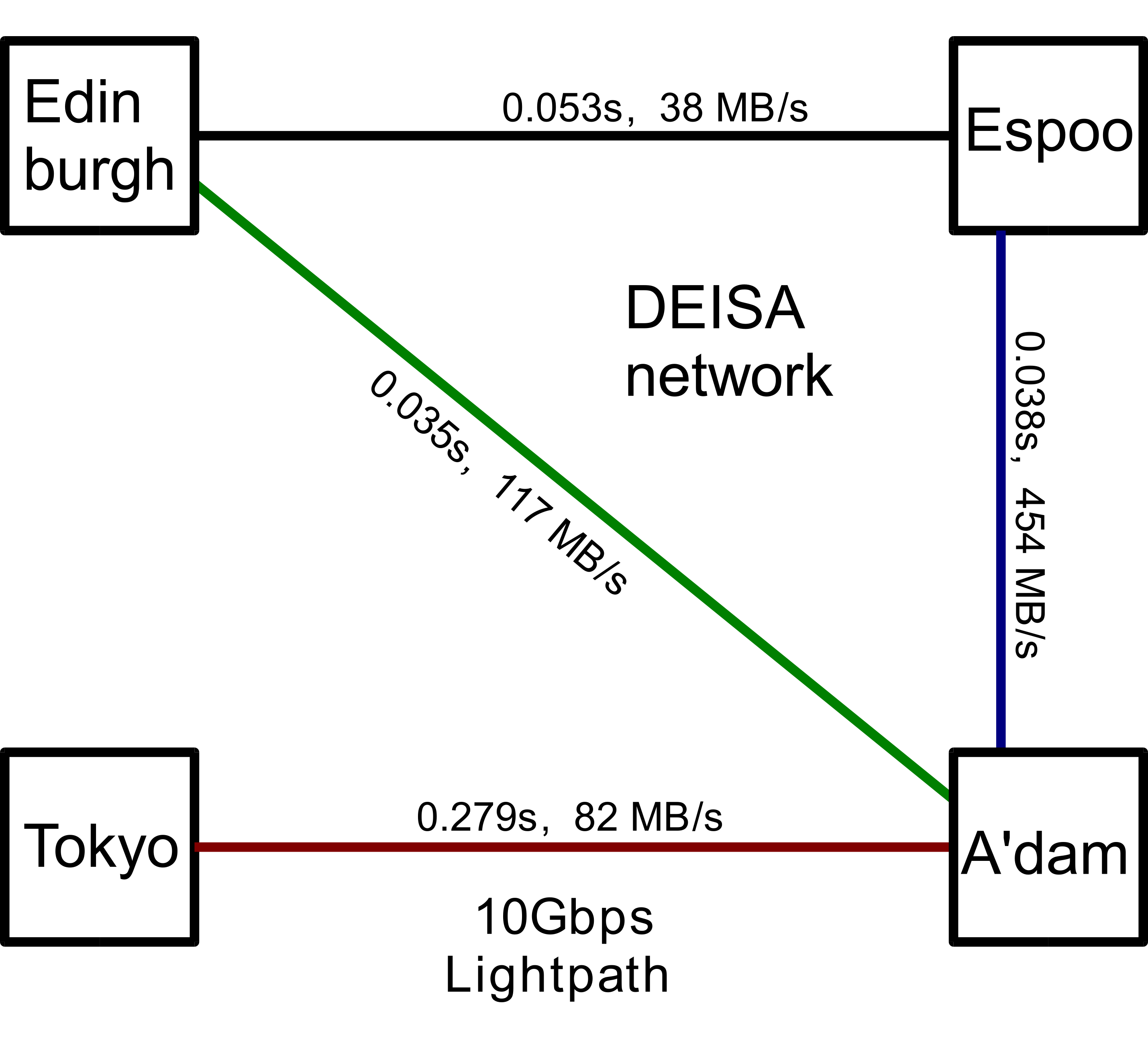
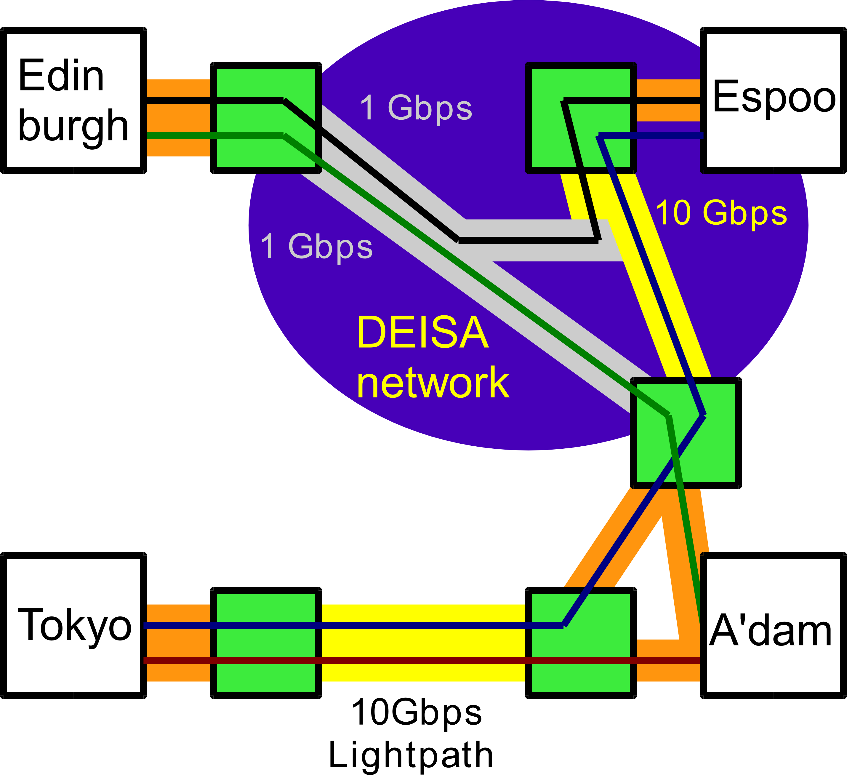
Figure 5: Network overview of a cosmological simulation across four supercomputers. The network latency and maximum sustained throughput for 64 MB message exchanges (using MPWide with the settings described in the text) over each network path is given on the left, and an overview of the network topology is given on the right. Here, the communication nodes are indicated by the solid green boxes.

4.4 GBBP results

The timing measurements of several simulations using $N=256^{3}$ are given in the right panel of Fig. 1 and 2 and measurements of simulations using $N=512^{3}$ are given in Fig. 7 and 8. We provide the timing results and model predictions for all our experiments in Tables 7 and 8.

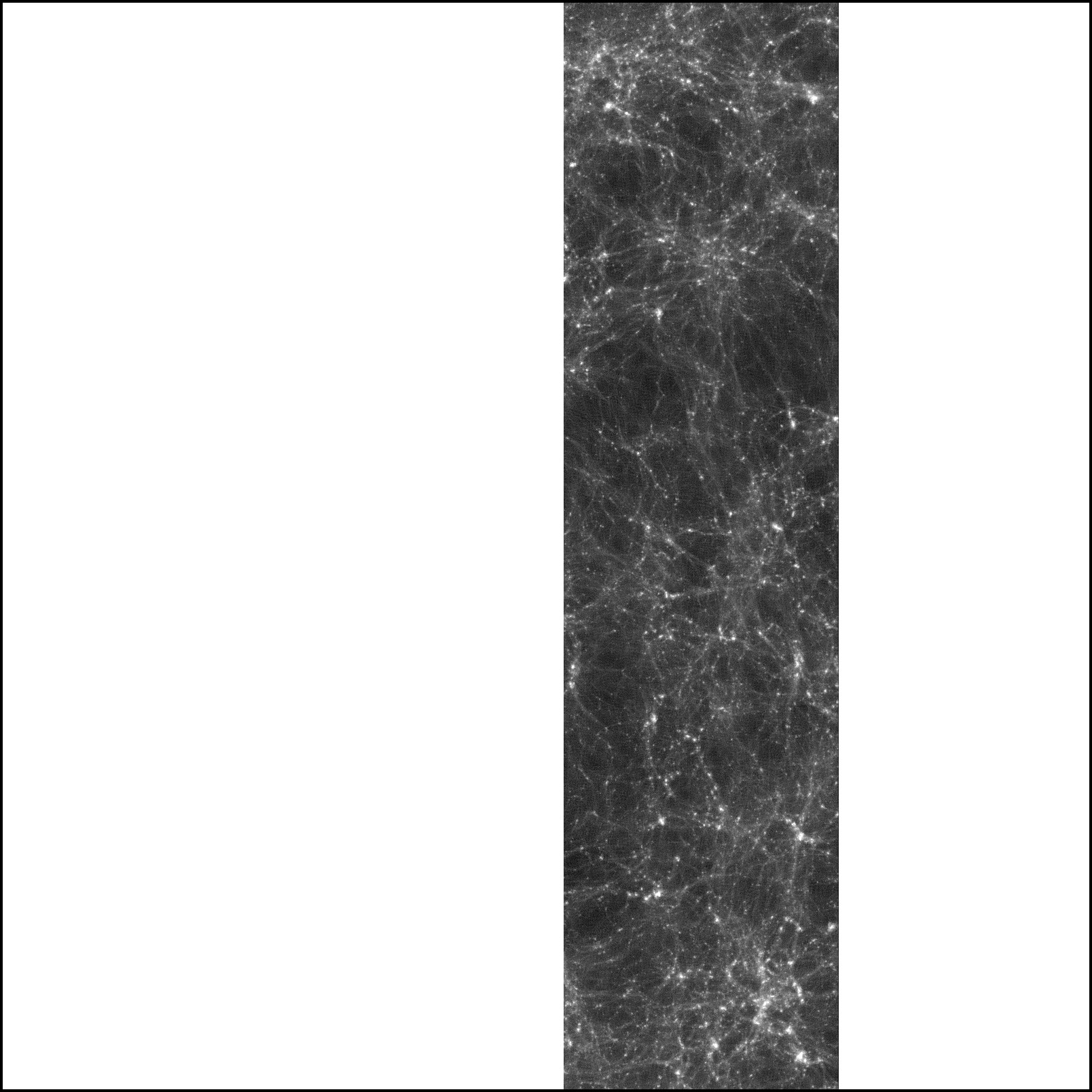
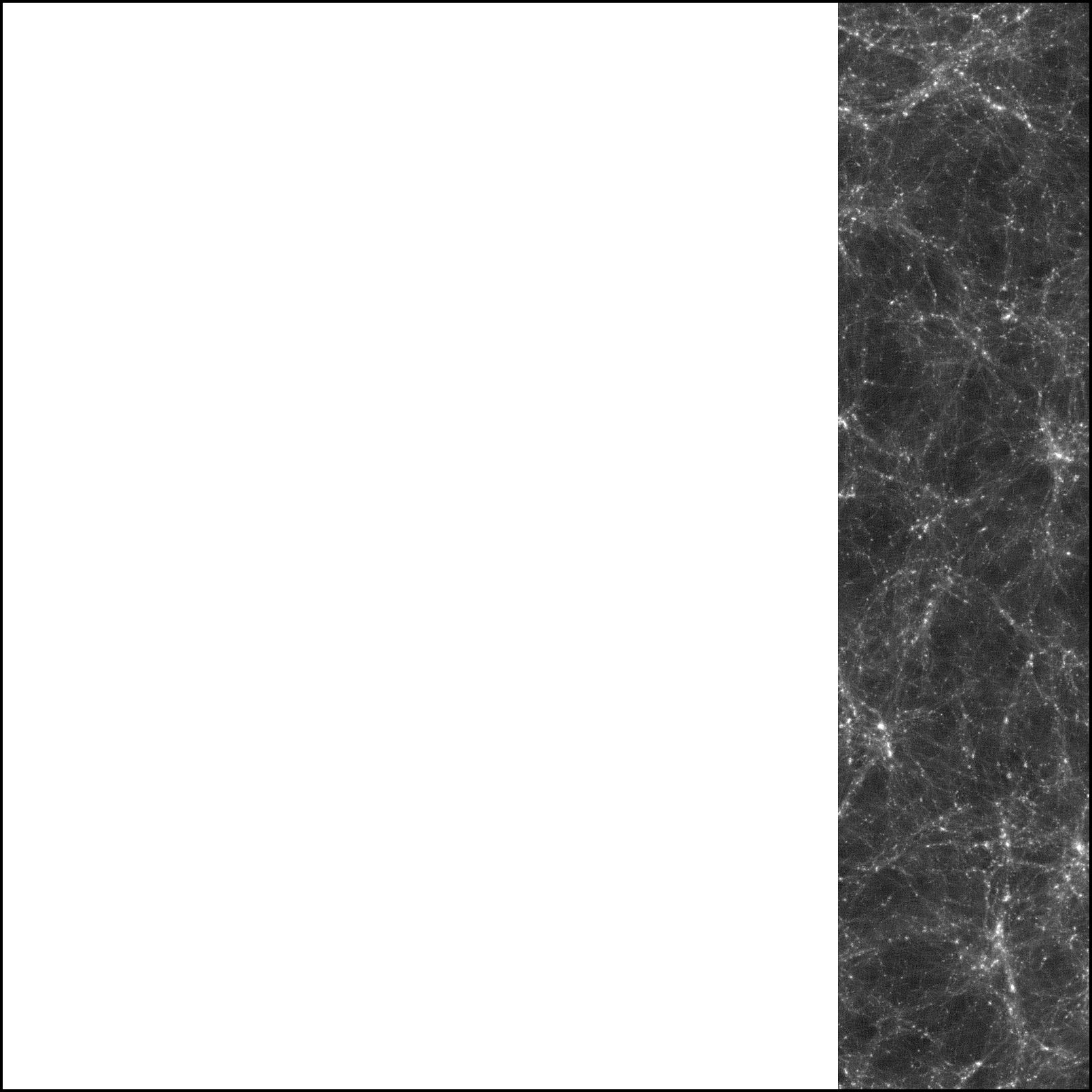
Figure 6: Snapshots at $z=5.65$ of a simulation with $N=512^{3}$ over four supercomputers. The slices have been placed to match the volumes on the supercomputers that reside respectively (from top left to bottom right) in Tokyo, Espoo, Edinburgh and Amsterdam.

Figure 7: As Fig. 3, but these simulations were run using 120 cores in total on the planet-wide network of supercomputers. The wall-clock time is given as a function of the number of supercomputers $s$. The average time spent on PM integration was 0.89-1.24 s for the runs using $M=128^{3}$, and 3.44-3.78 s for the runs using $M=256^{3}$. The ordering and technical specifications of the supercomputers we used are given in Tab. 5.

Figure 8: As Fig. 7, , but for simulations using $\theta=0.5$. The average time spent on PM integration was 0.89-1.24 s for the runs using $M=128^{3}$, and 3.44-3.78 s for the runs using $M=256^{3}$.

We have performed a number of runs with $N=256^{3}$ across up to three supercomputers. The runs over two supercomputers in the DEISA network have a communication overhead between 1.08 and 1.54 seconds. This constitutes between 8 and 13% of the total runtime for runs with $\theta=0.3$ and between 15 and 20% for runs with $\theta=0.5$. The run with $N=256^{3}$ between Edinburgh and Amsterdam has less communication overhead than the run between Espoo and Amsterdam, despite the 1 Gbps bandwidth limitation on the connection to Edinburgh. Our run between Amsterdam and Espoo suffered from a high background load, which caused the communication time to fluctuate over 10 steps with $\sigma\sim 0.25$ s, compared to $\sigma\sim 0.04$ s for the run between Amsterdam and Edinburgh. The run over three sites has a higher overhead than the runs over two sites, mainly due to using the direct connection between Edinburgh and Espoo, which is poorly optimized.

The wall-clock time of the simulations with $N=512^{3}$ is generally dominated by calculations, although the communication overhead becomes higher as we increase $s$. The runs over two sites (Espoo and Amsterdam) spend about 4-5 seconds on communication, which is less than 10 percent of the total execution time for the run using $\theta=0.3$. For simulations with $M=128^{3}$, the use of three supercomputers rather than two does not significantly increase the communication overhead. However, when we run simulations with $N=512^{3}$ and $M=256^{3}$ the use of a third supercomputer doubles the communication overhead. This increase in overhead can be attributed to the larger mesh size, as the now larger data volume of the mesh exchange scales with $s$.

We provide an overview of the time spent per simulation step for the run with $N=512^{3}$ and $M=128^{3}$ over three sites (Edinburgh, Espoo and Amsterdam) in Fig. 9. For this run the total communication overhead of the simulation code remains limited and relatively stable, achieving slightly lower values at later steps where $\theta=0.5$. A decomposition of the communication overhead for this run is given in the bottom panel of Fig. 9. The time required for exchanging the local essential tree constitutes about half of the total communication overhead. The simulation changes the opening angle at step 46, from $\theta=0.3$ to $\theta=0.5$. As a result, the size of the local essential tree becomes smaller and less time is spent on exchanging the local essential trees. The time spent on the other communications remains roughly constant throughout this run.

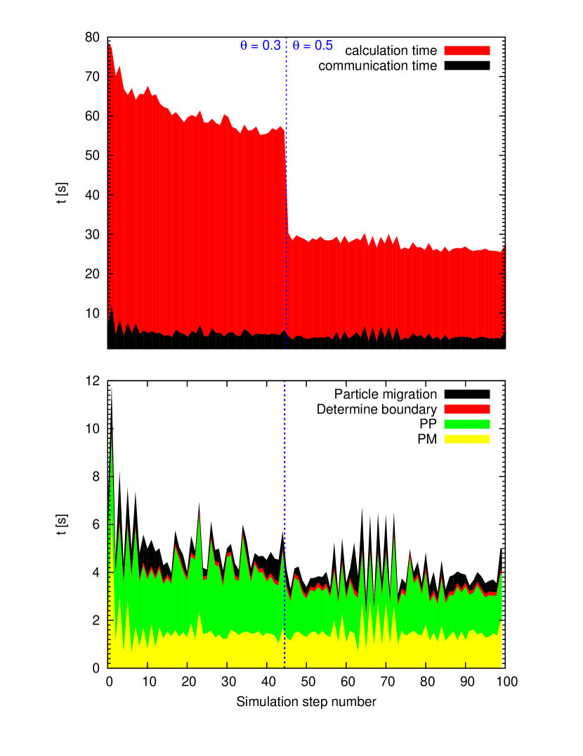
Figure 9: Performance results of a simulation with $N=512^{3}$ and $M=128^{3}$ using 120 processes in total across supercomputers in Amsterdam, Edinburgh and Espoo as a function of the simulation step number. The wall-clock time spent per step on calculations (top red area) and communications (bottom black area) is given in the top figure. Time spent on the four communication phases is given in the bottom figure. These phases are (from top to bottom) the migration of particles between sites, the exchanges of sample particles for determining the site boundaries, the local essential tree exchanges (PP) and the mesh cell exchanges (PM).

We have had a brief opportunity to run across all four supercomputers, which allowed us to run a simulation with $N=512^{3}$. We provide a density plot of the particle data present at each site at the end of this run in Fig. 6. In addition, the timing measurements of the run across four sites are given in the left panel of Fig. 7. Here we observe an increase in communication time from 3.8-4.8 seconds for a run over the three DEISA sites to 12.9-19.3 seconds for the run over all four sites. However, the runs over three sites relay messages between Edinburgh and Espoo through the supercomputer in Amsterdam, whereas the four site run uses the direct connection between these sites, which is poorly optimized. If we use the direct connection for a run across three sites the communication overhead increases from 3.8-4.8 seconds to 10.1-13.2 seconds per step (see Tables 7 and 8). Therefore, the communication overhead of a run across four sites may be reduced by a factor of two if we would relay the messages between Espoo and Edinburgh over Amsterdam.

$N^{1/3}$	$M^{1/3}$	np	$s$	comm.		tree	exec.	$t_{\rm comm}$		$t_{\rm tree}$	$t_{\rm exec}$
				local	total			only	$+w_{comm}$
				real	real	real	real	model	model	model	model
			#	[s]	[s]	[s]	[s]	[s]	[s]	[s]	[s]
256	128	60	A	0.207	0.207	11.32	11.80	0.04	0.03	10.79	11.22
256	128	60	HA	0.156	1.085	10.88	12.23	0.03	1.06	9.29	10.74
256	128	60	EA	0.177	1.536	10.91	12.71	0.03	1.06	9.39	10.84
256	128	60	AT	0.177	3.741	11.47	15.48	0.03	4.23	9.69	14.31
256	128	60	HEA*	0.143	5.960	10.95	17.12	0.03	1.66	8.86	10.91
512	128	120	A	1.045	1.045	69.57	71.04	0.06	0.06	58.98	59.91
512	128	120	HA	0.783	4.585	55.96	61.62	0.04	3.14	50.79	54.91
512	128	120	HEA	0.524	4.778	50.69	56.31	0.04	4.19	48.42	53.64
512	128	120	HEA*	0.760	13.17	56.82	71.01	0.04	4.19	48.42	53.64
512	128	120	HEAT*	0.653	19.26	49.96	70.10	0.04	9.42	48.06	58.52
512	256	120	A	1.367	1.367	42.13	46.04	0.16	0.16	49.60	52.46
512	256	120	HA	1.363	5.761	41.00	48.52	0.15	5.48	42.71	51.01
512	256	120	EA	1.247	7.091	37.60	46.37	0.15	5.48	43.17	51.47
512	256	120	AT	1.313	10.98	38.97	51.67	0.15	8.66	44.54	56.02
512	256	120	HEA	1.191	13.51	40.91	55.96	0.14	7.66	40.72	51.22
1024	256	240	E	3.215	3.215	182.4	189.6	0.20	0.20	200.7	205.8
1024	256	240	A	3.402	3.402	265.5	272.8	0.20	0.20	271.0	275.8
1024	256	240	HA	3.919	21.98	217.9	252.0	0.18	23.88	233.4	262.3
1024	256	240	HEA	4.052	31.28	258.0	294.7	0.17	26.05	217.1	248.4

Table 7: List of runs performed for GBBP that use $\theta=0.3$. The cube root of the number of particles and mesh cells are given in the first and second column, the number of processes and the supercomputers involved in the third and fourth column. Here, the letters correspond to supercomputers in Espoo (given by “H”), (E)dinburgh, (A)msterdam and (T)okyo. For runs over three and four sites, we relayed all traffic through the supercomputer in Amsterdam except for the runs marked with an asterisk, which used the direct network between Edinburgh and Espoo. The next four columns contain timing measurements from our experiments, which are average times per step averaged over 10 steps. The columns contain respectively the intra-site communication time, the total communication time, the time spent on tree integration (excluding PM) and the total wall-clock time. The last four columns contain the intra-site communication time, total communication time, tree integration time (excluding PM), and wall-clock time as predicted by our performance model.

$N^{1/3}$	$M^{1/3}$	np	$s$	comm.		tree	exec.	$t_{\rm comm}$		$t_{\rm tree}$	$t_{\rm exec}$
				local	total			only	$+w_{comm}$
				real	real	real	real	model	model	model	model
			#	[s]	[s]	[s]	[s]	[s]	[s]	[s]	[s]
256	128	60	A	0.197	0.197	5.968	6.446	0.04	0.04	5.42	5.84
256	128	60	HA	0.156	1.043	5.786	7.087	0.03	0.98	4.66	6.03
256	128	60	EA	0.159	1.480	5.827	7.567	0.03	0.98	4.71	6.08
256	128	60	AT	0.157	3.575	6.024	9.858	0.03	4.15	4.86	9.40
256	128	60	HEA*	0.143	5.827	6.047	12.08	0.03	1.58	4.45	6.41
512	128	120	A	0.992	0.992	34.31	35.76	0.05	0.05	29.59	30.52
512	128	120	HA	0.732	4.522	27.16	32.78	0.04	2.82	25.48	29.29
512	128	120	HEA	0.467	3.803	24.35	28.99	0.04	3.87	24.30	29.19
512	128	120	HEA*	0.760	10.86	28.52	40.45	0.04	3.87	24.30	29.19
512	128	120	HEAT*	0.534	12.90	25.84	39.68	0.03	9.09	24.11	34.25
512	256	120	A	1.308	1.308	22.91	26.80	0.16	0.16	24.89	27.74
512	256	120	HA	1.284	5.383	22.32	29.45	0.14	5.16	21.43	29.40
512	256	120	EA	1.213	6.991	20.75	29.44	0.14	5.16	21.66	29.63
512	256	120	AT	1.223	9.640	20.88	32.22	0.14	8.33	22.35	33.50
512	256	120	HEA	1.100	12.65	21.92	36.08	0.14	7.33	20.43	30.61
1024	256	240	HA	3.490	19.06	104.1	128.2	0.17	22.59	117.1	144.8
2048	256	750	AT	16.58	46.50	413.9	483.4	0.26	17.59	443.2	470.3

Table 8: As Tab. 7 but with $\theta=0.5$ instead of $\theta=0.3$. The run with $N=2048^{3}$ used an older version of the code and different settings, and is described in CosmoGrid .

We also ran several simulations with $N=1024^{3}$. The load balancing increases the communication volume of these larger runs considerably, as 850MB of particle data was exchanged on average during each step. However, the communication time still constitutes only one-tenth of the total run-time for the simulation across three supercomputers.

5 Scalability of $N$-body simulations across supercomputers

In this section we use our performance model and simulation results to predict the scalability of $N$-body code across grid sites. In the first part of this section we examine the predicted speedup and efficiency when scaling three cosmological $N$-body problems across multiple supercomputers. In the second part we apply existing performance models for tree codes (with block and shared time step schemes) and direct-method codes to predict the scalability of three stellar $N$-body problems across supercomputers. In the third part we predict the efficiency of cosmological $N$-body simulations over 8 sites as a function of the available bandwidth between supercomputers. We provide an overview of the three cosmological problems in Tab. 9, and an overview of the three stellar problems in Tab. 11.

Integrator	$N$	$M$	np 1	np 2
TreePM	$2048^{3}$	$256^{3}$	128	2048
TreePM	$2048^{3}$	$1024^{3}$	128	2048
TreePM	$8192^{3}$	$1024^{3}$	4096	32768

Table 9: Description of the cosmological $N$-body problems used for the scalability analysis across supercomputers. The type of integrator is given in the first column, the number of particles in the second column and the number of mesh cells in the third column. The last two columns contain respectively the number of processes per site for the speedup analysis and the number of total processes for the efficiency and bandwidth analysis.

These problems are mapped to a global grid infrastructure, which has a network latency of 0.3 s and a bandwidth capacity of 400 MB/s between supercomputers. The machine constants are similar to the ones we used for our runs, and can be found in Tab. 10. To limit the complexity of our analysis, we assume an identical calculation speed for all cores on all sites. Our performance predictions use an opening angle $\theta=0.5$.

Name of constant	Value	unit
$\tau_{\rm tree}$	$5.0\times 10^{-9}$	[s]
$\tau_{\rm fft}$	$3.5\times 10^{-9}$	[s]
$\tau_{\rm mesh}$	$7.5\times 10^{-7}$	[s]
$\lambda_{\rm lan}$	$8.0\times 10^{-5}$	[s]
$\lambda_{\rm wan}$	$3.0\times 10^{-1}$	[s]
$\sigma_{\rm lan}$	$2.3\times 10^{9}$	[bytes/s]
$\sigma_{\rm wan}$	$4.0\times 10^{8}$	[bytes/s]

Table 10: List of network parameters used for the scalability predictions of our code. The name of the constant can be found in the first column, the value used for our global grid model in the second column and the units used for each value in the third column.

5.1 Speedup and efficiency predictions for TreePM simulations

The predicted speedup $S(s)$ (as defined in Eq. 13) for three cosmological simulations as a function of the number of supercomputers $s$ can be found in Fig. 10. As the number of processes per site remains fixed, the total number of processes $p$ increases linearly with $s$. All example problems run efficiently over up to 3 sites. The simulation with $N=2048^{3}$ and $M=256^{3}$ scales well as $s$ increases and obtains a speedup of $\sim 13$ when $s=16$. When scaling up beyond $s\sim 25$, the speedup diminishes as the simulation becomes dominated by communication.

The simulation with $N=2048^{3}$ and $M=1024^{3}$ does not scale as well and only achieves a good speedup when run across a few sites. Here, the speedup as a function of $s$ begins to flatten at $s\sim 5$, due to the serial integration of the larger mesh. For $s\ {\raise-2.15277pt\hbox{$\buildrel>\over{\sim}$}}\ 16$, the communication overhead begins to dominate performance and the speedup decreases for higher $s$. The speedup of the run with $N=8192^{3}$ and $M=1024^{3}$ scales better with $s$ than the speedup of the run with $N=2048^{3}$ because it spends more time per step on tree force calculations.

We provide the predicted efficiency of three simulations over $s$ supercomputers relative to a simulation over one supercomputer, $E(s)$, using the same number of processes in Fig. 11. Here, the run with $N=2048^{3}$ and $M=256^{3}$ and the run with $N=8192^{3}$ and $M=1024^{3}$ retain a similar efficiency as we scale up with $s$. If $s\ {\raise-2.15277pt\hbox{$\buildrel>\over{\sim}$}}\ 6$, the run with $N=8192^{3}$ is slightly less efficient than the simulation with $N=2048^{3}$ and $M=256^{3}$. The simulation using $N=2048^{3}$ and $M=1024^{3}$ is less efficient than the other two runs. The data volume of the mesh cell exchange is 64 times higher than that of the run with $M=256^{3}$, which results in an increased communication overhead.

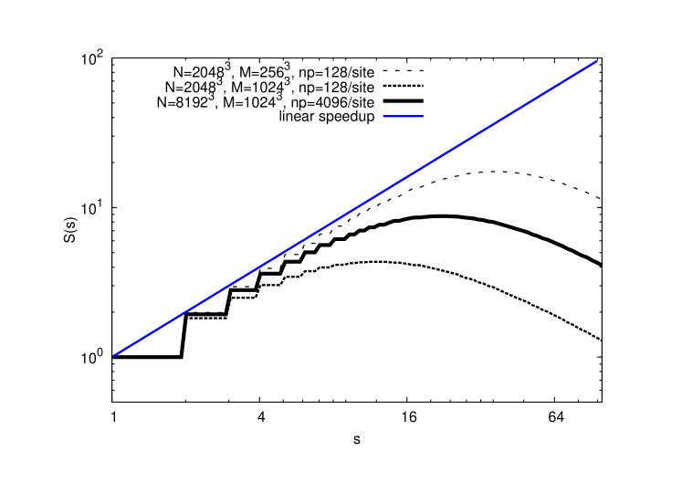
Figure 10: Predicted speedup $S(s)$ of simulations using the TreePM method as a function of the number of sites $s$ in a global grid. The total number of processes scales linearly with $s$.

Figure 11: Predicted efficiency $E(s)$ of simulations using the TreePM method as a function of the number of sites $s$ in a global grid. The total number of processes is kept fixed for all simulations.

5.2 Speedup and efficiency predictions for tree and direct-method simulations

We present predictions of three example $N$-body simulations of stellar systems, each of which uses a different integration method. The integration methods we use in our models are a Barnes-Hut tree algorithm 1986Natur.324..446B with shared time steps, a tree algorithm using block time steps 1986LNP…267…..H and a direct-method algorithm 1992PASJ…44..141M using block time steps. For the tree algorithm we choose the problem sizes and process counts previously used for the cosmological simulation models with $N=2048^{3}$. Modelling the performance of direct-method simulations using $N=2048^{3}$ is unrealistic, because one step of force calculations for the $2048^{3}$ particles would already take $sim$ 280 years when using 1000 nodes on a PC cluster Gualandris2007 . We instead predict the performance of direct-method simulations using a more realistic problem size of 5 million particles.

We model the tree algorithm using a slightly extended version of the models presented in 2004PASJ…56..521M ; 1991PASJ…43..621M and the direct-method algorithm using the grid-enabled model presented in 2008NewA…13..348G . An overview of the three problems used for our predictions is given in Tab. 11.

Integrator	$N$	np 1	np 2	time step scheme
Tree	$2048^{3}$	128	2048	shared
Tree	$2048^{3}$	128	2048	block
Direct	$5\cdot 10^{6}$	16	128	block

Table 11: Description of the stellar $N$-body problems used for the scalability analysis across supercomputers. The type of integrator is given in the first column and the number of particles in the second column. The number of processes per site for respectively the speedup analysis and the efficiency analysis are given in the third and fourth column. The time step scheme used is given in the last column. Note that the direct-method simulation is modelled for a grid of GPUs.

The simulations using the tree algorithm are mapped to the same global grid infrastructure that we used for modelling the cosmological simulation (see Tab. 10 for the machine constants used). The direct-method simulation is modelled using the network constants from the global grid model, but here we assume that each node has a Graphics Processing Unit (GPU) with a force calculation performance of 200 GFLOP/s. As each force interaction requires 66 FLOPs on a GPU, we spend $3.3\times 10^{-10}$s per force interaction (see 2007NewA…12..641P ; 2009NewA…14..630G for details on direct $N$-body integration on the GPU).

5.2.1 Performance model for the tree algorithm

We extend the tree code models given in 2004PASJ…56..521M ; 1991PASJ…43..621M to include the grid communication overhead by adding the equations for wide area communication of the tree method from our SUSHI performance model. In accordance with our previous model, we define the wide area latency-bound time for the tree method ($w_{\rm l,tree}$) as,

$$w_{\rm l,tree} = \lambda_{\rm wan}\left(4\left(s-1\right)+4\right).$$ (15)

The bandwidth-bound communication time ($w_{\rm b,tree}$) consists of the communication volume for the local essential tree exchange, which we estimate to be double the size used in TreePM simulations due to the lack of PM integration, and the communication volume required for particle sampling. It is therefore given by,

$$w_{\rm b,tree} = \frac{\left(96/\theta+48\right)N^{2/3}+4Nr_{\rm samp}}{\sigma_{\rm wan}},$$ (16)

where $r_{\rm samp}=1/10000$ and $\theta=0.5$. We use the equation given in 1991PASJ…43..621M for Plummer sphere data sets to calculate the total number of force interactions.

5.2.2 Modelling of block time steps

Tree and direct $N$-body integrators frequently use a block time step scheme instead of a shared time step scheme. Block-time step schemes can also be applied to parallel simulations (unlike e.g., individual time step schemes), and reduce the computational load by integrating only a subset of particles during each step 1986LNP…267..233H ; 1991ApJ…369..200M . To equalize the number of integrated particles between simulations, we therefore compare a single shared time-step integration with $N/n_{\tt b}$ steps of a block time-step integration, where $n_{\tt b}$ is the average block size. We adopt an average block size of $n_{\tt b}=0.2N^{0.81}$ for all block time-step integrators, the same value that was used in 2008NewA…13..348G .

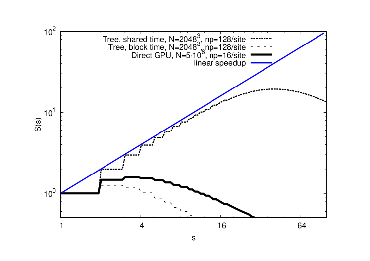
Figure 12: Predicted speedup $S(s)$ of $N$-body simulations using the tree and direct method as a function of the number of sites $s$ in a global grid. The total number of processes scales linearly with $s$.

5.2.3 Predictions

We give the predicted speedup $S(s)$ of the three simulations as a function of the number of supercomputers $s$ in Fig. 12. Here, the tree code with shared time steps scales similarly to the cosmological simulation with $N=2048^{3}$ and $M=256^{3}$ (see Fig. 10). We predict a speedup of $\sim 13$ when $s=16$. When we model the tree code with a block time step scheme, the scalability becomes worse because it requires $N/n_{\tt b}$ times as many communication steps to integrate $N$ particles. The large number of communications combined with the high latency of wide area networks result in a high communication overhead. The direct $N$-body run on a global grid of GPUs also does not scale well over $s$ due to the use of block time steps.

We give the predicted efficiency of the three simulations over $s$ supercomputers relative to a simulation over one supercomputer, $E(s)$ in Fig. 13. The efficiency of these runs is mainly limited by the latency-bound communication time. The tree code with shared time steps retains a high efficiency for $s\ {\raise-2.15277pt\hbox{$\buildrel<\over{\sim}$}}\ 16$, while the simulations with block time steps are less efficient due to the larger number of communications. We predict a slightly higher efficiency when $s\ {\raise-2.15277pt\hbox{$\buildrel>\over{\sim}$}}\ 4$ for the direct-method simulation than for the tree code simulation with block time steps. This is because the lower $N$ results in a lower number of communication steps, and therefore in less communication overhead.

Figure 13: Predicted efficiency $E(s)$ of $N$-body simulations using the tree and direct method as a function of the number of sites $s$ in a global grid. The total number of processes is kept fixed for all simulations.

5.3 Bandwidth analysis for cosmological simulations

We have shown that our TreePM code scales well across up to $\sim 16$ sites if the ratio between the number of particles and the number of mesh cells is sufficiently large. Here we examine the efficiency of four cosmological simulations over 8 sites. The efficiency compared to a single site run is predicted as a function of the available bandwidth. We have included three predictions for a global grid with 0.3 s network latency as well as one prediction for a simulation with $N=2048^{3}$ and $M=256^{3}$ over a medium-range grid with 30 ms network latency. The details of these simulations are given in Tab. 9, and the results are shown in Fig. 14.

We find that the efficiency of cosmological simulations across sites is heavily dependent on the available bandwidth. The run with $N=2048^{3}$ and $M=256^{3}$ on a global grid has $E(8)=0.9$ (where $E(8)$ is the efficiency as defined in Eq. 14) when the supercomputers are connected with a 100 MB/s network. Using a network with a higher bandwidth has little effect on the achieved efficiency, as the communication overhead is then dominated by network latency. The effect of network latency is clearly visible when we look at the prediction for the same simulation on a grid with a shorter baseline. When using a grid with 30 ms network latency the simulation reaches $E(8)=0.97$ if the wide area network achieves a throughput of 1000 MB/s (which is possible with a fine-tuned and dedicated 10 Gbps optical network). We predict an efficiency $E(8)>0.8$ for both simulations if the available network bandwidth between sites is 50 MB/s.

The run with $N=2048^{3}$ and $M=1024^{3}$ is more communication intensive, and requires a network throughput of at least 700 MB/s to achieve an efficiency of 0.8. The simulation using $N=8192^{3}$ and $M=1024^{3}$ runs more efficiently than the simulation using $N=2048^{3}$ and $M=1024^{3}$ independent of the obtained bandwidth. Although the exchanged data volume is larger in the run with $N=8192^{3}$, this increased overhead is offset by the the higher force calculation time per step. The large communication volume reduces the efficiency considerably for low bandwidth values, and an average network throughput of at least 150 MB/s is required to achieve an efficiency of $E(8)=0.8$.

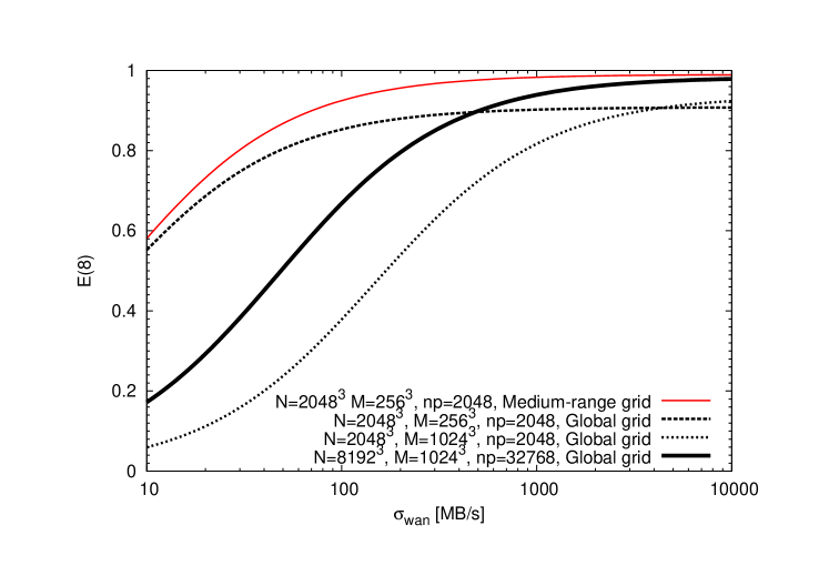
Figure 14: Predicted efficiency of four $N$-body simulations using the TreePM method over 8 sites ($E(8)$) as a function of the wide area network throughput ($\sigma_{wan}$) in MB/s. Three simulations are run on a global grid. One simulation uses $N=2048^{3}$ particles and $M=256^{3}$ mesh cells (given by the black dashed line), one uses $N=2048^{3}$ and $M=1024^{3}$ (black dotted line) and one run uses $N=8192^{3}$ and $M=1024^{3}$ (thick black line). A simulation using $N=2048^{3}$ and $M=256^{3}$ modelled for a grid with 30 ms network latency between sites is given by the thin red line. Runs with $N=2048^{3}$ particles are predicted using a total of 2048 processes, runs with $N=8192^{3}$ particles are predicted using a total of 32768 processes.

6 Conclusion

We have run a few dozen cosmological $N$-body simulations and analyzed the scalability of our SUSHI integrator on a national distributed computer and across a global network of supercomputers. Our results confirm that SUSHI is able to efficiently perform simulations across supercomputers. We were able to run a simulation using $1024^{3}$ particles across three supercomputers with $\sim 10\%$ communication overhead. The communication performance can be further improved by tuning the optical networks.

Based on our model predictions we conclude that a long-term cosmological simulation using $2048^{3}$ particles and $256^{3}$ mesh cells scales well over up to $\sim 16$ sites, given that sufficient bandwidth is available and the number of cores used per site is limited to $\sim 256$. We also predict that tree codes with a shared time step scheme run efficiently across multiple supercomputers, while tree codes with a block time step scheme do not.

Considerable effort is still required to obtain acceptable message passing performance through a long distance optical network. This is due to three reasons. First, it may take up to several months to arrange an intercontinental light path. Second, optical networks are generally used for high volume data streaming such as distributed visualization or bulk data transfer, and are therefore not yet tuned to achieve optimal message passing performance. Third, intercontinental networks traverse a large number of different institutes, making it politically difficult for users to diagnose and adjust settings on individual sections of the path. For our experiments we therefore chose to optimize the wide area communications by tuning our application, rather than requesting system-level modifications to the light path configuration.

The main challenges in running simulations across supercomputers are now political, rather than technical. During the GBBP project, we were able to overcome many of the political challenges in part due to good will of all organizations involved and in part through sheer patience and perseverance. However, orchestrating a reservation spanning across multiple supercomputers is a major political undertaking. The use of a meta-scheduler and reservation system for supercomputers and optical networks greatly reduces this overhead, and also improves the workload distribution between supercomputer centers. Once the political barriers are overcome, we will be able to run long lasting and large scale production simulations over a grid of supercomputers.

References

- [1] E. Fernandez, E. Heymann, and M. Angel Senar. Supporting efficient execution of mpi applications across multiple sites. In Euro-Par 2006 Parallel Processing, pages 383–392. Springer, 2006.
- [2] A. Gualandris, S. Portegies Zwart, and A. Tirado-Ramos. Performance analysis of direct n-body algorithms for astrophysical simulations on distributed systems. Parallel Computing, 33(3):159–173, 2007.
- [3] S. Manos, M. Mazzeo, O. Kenway, P. V. Coveney, N. T. Karonis, and B. R. Toonen. Distributed mpi cross-site run performance using mpig. In HPDC, pages 229–230, 2008.
- [4] H. Bal and K. Verstoep. Large-scale parallel computing on grids. Electronic Notes in Theoretical Computer Science, 220(2):3 – 17, 2008. Proceedings of the 7th International Workshop on Parallel and Distributed Methods in verifiCation (PDMC 2008).
- [5] P. Bar, C. Coti, D. Groen, T. Herault, V. Kravtsov, M. Swain, and A. Schuster. Running parallel applications with topology-aware grid middleware. In Fifth IEEE international conference on e-Science and Grid computing: Oxford, United Kingdom, pages 292–299, Piscataway, NJ, December 2009. IEEE Computer Society.
- [6] M. Norman, P. Beckman, G. Bryan, J. Dubinski, D. Gannon, L. Hernquist, K. Keahey, J. Ostriker, J. Shalf, J. Welling, and S. Yang. Galaxies Collide On the I-Way: an Example of Heterogeneous Wide-Area Collaborative Supercomputing. International Journal of High Performance Computing Applications, 10(2-3):132–144, 1996.
- [7] T. J. Pratt, L. G. Martinez, M. O. Vahle, and T. V. Archuleta. Sandia‘s network for supercomputer ‘96: Linking supercomputers in a wide area asynchronous transfer mode (atm) network. Technical report, Sandia National Labs., Albuquerque, NM (United States), 1997.
- [8] C. Stewart, R. Keller, R. Repasky, M. Hess, D. Hart, M. Muller, R. Sheppard, U. Wossner, M. Aumuller, H. Li, D. Berry, and J. Colbourne. A global grid for analysis of arthropod evolution. In GRID ’04: Proceedings of the 5th IEEE/ACM International Workshop on Grid Computing, pages 328–337, Washington, DC, USA, 2004. IEEE Computer Society.
- [9] S. Portegies Zwart, T. Ishiyama, D. Groen, K. Nitadori, J. Makino, C. de Laat, S. McMillan, K. Hiraki, S. Harfst, and P. Grosso. Simulating the universe on an intercontinental grid. Computer, 43:63–70, 2010.
- [10] K. Yoshikawa and T. Fukushige. PPPM and TreePM Methods on GRAPE Systems for Cosmological N-Body Simulations. Publications of the Astronomical Society of Japan, 57:849–860, December 2005.
- [11] G. Xu. A New Parallel N-Body Gravity Solver: TPM. ApJS, 98:355–366, May 1995.
- [12] J. Barnes and P. Hut. A Hierarchical O(NlogN) Force-Calculation Algorithm. Nature, 324:446–449, December 1986.
- [13] R. W. Hockney and J. W. Eastwood. Computer Simulation Using Particles. New York: McGraw-Hill, 1981, 1981.
- [14] K. Nitadori, J. Makino, and P. Hut. Performance tuning of N-body codes on modern microprocessors: I. Direct integration with a hermite scheme on x86_64 architecture. New Astronomy, 12:169–181, December 2006.
- [15] Matteo Frigo, Steven, and G. Johnson. The design and implementation of fftw3. In Proceedings of the IEEE, volume 93, pages 216–231, Feb 2005.
- [16] T. Ishiyama, T. Fukushige, and J. Makino. GreeM: Massively Parallel TreePM Code for Large Cosmological N -body Simulations. Publications of the Astronomical Society of Japan, 61:1319–1330, December 2009.
- [17] J. Makino. A Fast Parallel Treecode with GRAPE. Publications of the Astronomical Society of Japan, 56:521–531, June 2004.
- [18] D. Groen, S. Rieder, P. Grosso, C. de Laat, and P. Portegies Zwart. A light-weight communication library for distributed computing. Computational Science and Discovery, 3(1):015002, 2010.
- [19] DAS-3. The distributed asci supercomputer 3: http://www.cs.vu.nl/das3/.
- [20] S. L. W. McMillan. The use of supercomputers in stellar dynamics; proceedings of the workshop, institute for advanced study, princeton, nj, june 2-4, 1986. In P. Hut and S. L. W. McMillan, editors, The Use of Supercomputers in Stellar Dynamics, volume 267 of Lecture Notes in Physics, Berlin Springer Verlag, page 156, 1986.
- [21] J. Makino and S. J. Aarseth. On a Hermite integrator with Ahmad-Cohen scheme for gravitational many-body problems. Publications of the Astronomical Society of Japan, 44:141–151, April 1992.
- [22] J. Makino. Treecode with a Special-Purpose Processor. Publications of the Astronomical Society of Japan, 43:621–638, August 1991.
- [23] D. Groen, S. Portegies Zwart, S. McMillan, and J. Makino. Distributed N-body simulation on the grid using dedicated hardware. New Astronomy, 13:348–358, July 2008.
- [24] S. F. Portegies Zwart, R. G. Belleman, and P. M. Geldof. High-performance direct gravitational N-body simulations on graphics processing units. New Astronomy, 12:641–650, November 2007.
- [25] E. Gaburov, S. Harfst, and S. Portegies Zwart. SAPPORO: A way to turn your graphics cards into a GRAPE-6. New Astronomy, 14:630–637, October 2009.
- [26] D. C. Heggie and R. D. Mathieu. Standardised Units and Time Scales. In P. Hut and S. L. W. McMillan, editors, The Use of Supercomputers in Stellar Dynamics, volume 267 of Lecture Notes in Physics, Berlin Springer Verlag, page 233, 1986.
- [27] J. Makino. Optimal order and time-step criterion for Aarseth-type N-body integrators. ApJ, 369:200–212, March 1991.