A Beaming-Independent Estimate of the Energy Distribution of Long Gamma-Ray Bursts: Initial Results and Future Prospects

Abstract

We present single-epoch radio afterglow observations of $24$ long-duration gamma-ray burst (GRB) on a timescale of $\gtrsim 100$ d after the burst. These observations trace the afterglow evolution when the blastwave has decelerated to mildly- or non-relativistic velocities and has roughly isotropized. We infer beaming-independent kinetic energies using the Sedov-Taylor self-similar solution, and find a median value for the sample of detected bursts of about $7\times 10^{51}$ erg, with a $90\%$ confidence range of $1.1\times 10^{50}-3.3\times 10^{53}$ erg. Both the median and $90\%$ confidence range are somewhat larger than the results of multi-wavelength, multi-epoch afterglow modeling (including large beaming corrections), and the distribution of beaming-corrected $\gamma$-ray energies. This is due to bursts in our sample with only a single-frequency observation for which we can only determine an upper bound on the peak of the synchrotron spectrum. This limitation leads to a wider range of allowed energies than for bursts with a well-measured spectral peak. Our study indicates that single-epoch centimeter-band observations covering the spectral peak on a timescale of $\delta t\sim 1$ yr can provide a robust estimate of the total kinetic energy distribution with a small investment of telescope time. The substantial increase in bandwidth of the EVLA (up to 8 GHz simultaneously with full coverage at $1-40$ GHz) will provide the opportunity to estimate the kinetic energy distribution of GRBs with only a few hours of data per burst.

1. Introduction

The energy budget of gamma-ray bursts (GRBs) provides fundamental insight into the nature of the explosions, the resulting ejecta properties, and the identity of the central compact remnant (“engine”). While the isotropic-equivalent $\gamma$-ray energy ($E_{\rm\gamma,iso}$) can be easily determined from a measurement of the burst fluence and redshift, a complete accounting of the energy budget requires detailed observations of the afterglow emission. The afterglow observations provide a measure of the isotropic-equivalent blastwave kinetic energy ($E_{\rm K,iso}$), as well as the explosion geometry (quantified by a jet opening angle, $\theta_{j}$). The resulting beaming corrections, $f_{b}^{-1}\equiv 1-{\rm cos}(\theta_{j})$, can be substantial, approaching three orders of magnitude in some cases (Frail et al., 2001; Panaitescu & Kumar, 2002; Berger et al., 2003a; Bloom et al., 2003). To properly determine $E_{\rm K,iso}$ and $f_{b}$ it is essential to observe the afterglows from radio to X-rays over timescales of hours to weeks, clearly a challenging task. This is particularly a problem for the subset of “dark” GRBs for which the lack of detected optical emission, or large extinction, prevent a determination of $E_{\rm K,iso}$ and likely $f_{b}$ (e.g., Berger et al. 2002; Piro et al. 2002).

Over the past decade detailed afterglow observations have been obtained at a great cost of telescope time for about $20$ long-duration GRBs, with the basic result that the beaming corrections are large and diverse, leading to typical true energies of $E_{\gamma}\sim E_{K}\sim 10^{51}$ erg (Frail et al., 2001; Panaitescu & Kumar, 2001, 2002; Berger et al., 2003a, b; Bloom et al., 2003). More recently, it has been recognized that some nearby long GRBs have much lower energies, $E_{\rm iso}\sim 10^{49}-10^{50}$ erg, and appear to be quasi-isotropic (Kulkarni et al., 1998; Soderberg et al., 2004b, 2006). Similarly, some bursts appear to have large beaming-corrected energies of $\sim 10^{52}$ erg (Cenko et al., 2010b, a). The existence of these highly energetic bursts depends at least in part on the ability to correctly infer their large beaming corrections. Indeed, the inference of jet opening angles from breaks in the afterglow light curves has become controversial in recent years due to conflicting trends in optical and X-ray light curves (Liang et al., 2008; Racusin et al., 2009). Similarly, in some cases a two-component jet has been inferred, with a narrow core dominating the $\gamma$-ray emission and a wider component dominating the afterglow emission (Berger et al., 2003b; Racusin et al., 2008). Numerical simulations suggest that off-axis viewing angles can also lead to shallow breaks that may be missed or mis-interpreted (van Eerten et al., 2010).

In addition to potential difficulties with the inference of $f_{b}$, the $\gamma$-ray and kinetic energies measured from the early afterglow emission only pertain to the relativistic ejecta. The existence of a substantial component of mildly relativistic ejecta can only be determined from observations at late times when such putative material can refresh the forward shock. Clearly, the existence of substantial energy in a slow ejecta component will place crucial constraints on the activity lifetime of the central engine.

Such late-time observations also have the added advantage that they probe the blastwave when it has decelerated to non-relativistic velocities and hence roughly approaches isotropy (Frail et al., 2000; Livio & Waxman, 2000). This allows us to use the well-established Sedov-Taylor self-similar solution, with negligible beaming corrections, to estimate the total kinetic energy of both the decelerated ejecta and any additional initially non-relativistic material. Since the peak of the afterglow spectrum on these timescales is located in the radio band, the lack of optical afterglow emission (e.g., due to extinction) does not have an effect on the ability to determine $E_{K}$.

This approach was first exploited by Frail et al. (2000) to model the late-time radio afterglow emission of GRB 970508 (at $\delta t\gtrsim 100$ d) from which the kinetic energy was inferred to be $E_{K}\sim 5\times 10^{50}$ erg. Berger et al. (2004) used the same approach to model the radio afterglow emission of GRB 980703 on timescales of $\gtrsim 40$ d, and to re-model GRB 970508. They found kinetic energies of $E_{K}\sim 3\times 10^{51}$ erg for both bursts. Finally, Frail et al. (2005) modeled the radio emission from GRB 030329 at $\delta t\gtrsim 50$ d and found $E_{K}\sim 10^{51}$ erg. Only 3 bursts have been studied in this fashion so far because only those events have well-sampled radio light curves on the relevant timescales of $\delta t\gtrsim 100$ d.

However, the kinetic energy can still be estimated using the same methodology even from fragmentary late-time radio observations. Such an approach will naturally result in larger uncertainties for each burst, but it can be applied to a much larger sample of events. Here we present such an analysis for $24$ long-duration GRBs with radio observations at $\gtrsim 100$ d, but with only $1-3$ data points (at 1.4 to 8.5 GHz) per burst. Using these observations we infer robust ranges for the kinetic energy of each burst and for the population as a whole. The plan of the paper is as follows. The radio observations are summarized in §2. The model for synchrotron emission from a Sedov-Taylor blastwave, and the various assumptions we employ are presented in §3. In §4 we detail the resulting kinetic energies and the range for the overall sample, and we compare these results to multi-wavelength analyses of early afterglows in §5. We conclude with a discussion of future prospects.

2. Radio Data

We use radio observations of $24$ long GRBs at $\delta t\gtrsim 100$ d since on those timescales the blastwave is expected to become non-relativistic and roughly isotropic (Livio & Waxman, 2000), and the peak of the afterglow emission is at or below the centimeter band. This has been confirmed with detailed data in the case of GRBs 970508, 980703, and 030329 (Frail et al., 2000; Berger et al., 2004; Frail et al., 2005). We restrict the analysis to GRBs with a known redshift and with early-time detections, which for the case of a single detection or upper limit allow us to infer that the peak of the spectrum has transitioned below our observing frequency.

The observations are primarily from the Very Large Array (VLA), with the exception of GRBs 980425 and 011121 which were observed with the Australia Telescope Compact Array (ATCA). The data were obtained between 1997 and 2009 as part of a long-term GRB radio program (e.g., Frail et al. 2003a).

For the purpose of our analysis, we separate the bursts into three categories based on the quality of the data. In Group A are 3 bursts with late-time detections at multiple frequencies that constrain the peak of the synchrotron spectrum (the same three bursts that have been studied in detail by Frail et al. 2000; Berger et al. 2004; Frail et al. 2005). In Group B are 11 bursts with single-frequency detections, while Group C consists of 10 GRBs with late-time non-detections. The VLA measurements and relevant burst properties are listed in table 1.

3. Synchrotron Emission from a Non-Relativistic Blastwave

Our modeling of the radio data follows the methodology of Frail et al. (2000) and Berger et al. (2004) for the case of a uniform density medium. For the typical expected parameters of long GRBs, the initially collimated blastwave approaches spherical symmetry and decelerates to non-relativistic velocity on similar timescales, $t_{s}\approx 150(E_{\rm K,iso,52}/n_{e})^{1/4}t_{\rm j,d}^{1/4}$ d and $t_{NR}\approx 40(E_{\rm K,iso,52}/n_{e})^{1/4}t_{\rm j,d}^{1/4}$ d, respectively (Livio & Waxman, 2000); here, $n_{e}$ is the circumburst density in units of cm^-3 and $t_{j}$ is the “jet break” time at which the jet begins to expand sideways (i.e., $\Gamma(t_{j})\sim\theta_{j}^{-1}$, where $\Gamma$ is the bulk Lorentz factor). In this paper we assume that the blastwave has transitioned to the non-relativistic isotropic phase by the time of our observations and subsequently check for self-consistency.

The blastwave dynamics in the non-relativistic phase are described by the Sedov-Taylor self-similar solution with $r(t)\propto(E_{\rm ST}t^{2}/n)^{1/5}$. To calculate the synchrotron emission emerging from the shock-heated material, we make the usual assumptions: (i) the electrons are accelerated to a power-law energy distribution, $N(\gamma)\propto\gamma^{-p}$ for $\gamma>\gamma_{m}$, where $\gamma_{m}$ is the minimum Lorentz factor; (ii) the value of $p$ is 2.2 as inferred from several bursts (e.g., Panaitescu & Kumar 2001, 2002; Yost et al. 2003); and (iii) the energy densities in the magnetic field and electrons are constant fractions ($\epsilon_{B}$ and $\epsilon_{e}$, respectively) of the shock energy density. Accounting for synchrotron emissivity and self-absorption, and including the appropriate redshift transformations, the flux observed at frequency $\nu$ and time $t$ is given by (Frail et al., 2000; Berger et al., 2004):

$$F_{\nu}=F_{0}(t/t_{0})^{\alpha_{F}}[(1+z)\nu]^{5/2}(1-e^{-\tau_{\nu}})f_{3}(\nu/\nu_{m})f^{-1}_{2}(\nu/\nu_{m}),$$ (1)

where the optical depth is given by:

$$\tau_{\nu}=\tau_{0}(t/t_{0})^{\alpha_{\tau}}[(1+z)\nu]^{-(p+4)/2}f_{2}(\nu/\nu_{m}),$$ (2)

the synchrotron peak frequency, corresponding to electrons with $\gamma=\gamma_{m}$, is given by:

$$\nu_{m}=\nu_{0}(t/t_{0})^{\alpha_{m}}(1+z)^{-1},$$ (3)

and the function $f_{l}(x)$ is given by

$$f_{l}(x)=\int^{x}_{0}F(y)y^{(p-l)/2}\,dy,$$ (4)

where $F(y)$ is an integration over Bessel functions (Rybicki & Lightman, 1979). The temporal indices in the case of a uniform density medium are $\alpha_{F}=11/10$, $\alpha_{\tau}=1-3p/2$, and $\alpha_{m}=-3$. The normalizations are such that $F_{0}$ and $\tau_{0}$ are the flux density and optical depth at a frequency of $\nu=1$ Hz at $t=t_{0}$, and $\nu_{0}$ is the synchrotron peak frequency in the rest frame of burst at $t=t_{0}$. Furthermore, the synchrotron self-absorption frequency, $\nu_{a}$, is defined by the condition $\tau_{\nu}(\nu_{a})=1$.

We fit this synchrotron model to our radio data using $F_{0}$, $\tau_{0}$, and $\nu_{0}$ as free parameters. Since we have no a priori knowledge about the expected values of the synchrotron spectrum parameters we assume that they follow a flat distribution in log-space. We note that any further assumption about the distribution of these parameters will only serve to restrict the resulting energy distributions, and we therefore consider our assumed flat distribution to be conservative. For the detected objects (Groups A and B) we retain all solutions that reproduce the measured flux density within the error bars, while for the non-detections we use $3\sigma$ as an upper bound. Moreover, for the bursts in Group A, $\nu_{0}$ is constrained by the multi-frequency observations and no additional constraints are required. However, for the bursts in Groups B and C, which have only a single-frequency observation, we require that both $\nu_{m}$ and $\nu_{a}$ have values below the observing frequency since the light curves are always declining at the time of our observations.

Using the allowed ranges of $F_{0}$, $\tau_{0}$, and $\nu_{0}$ we determine the set of relevant physical parameters: $n_{e}$, $\gamma_{m}$, and $B$, where $B$ is the magnetic field strength. The radius of the blastwave, $r$, remains unconstrained (e.g., Frail et al. 2000; Berger et al. 2004):

$$B=11.7(p+2)^{-2}F^{-2}_{0,-52}(r_{17}/d_{L,28})^{4}\,\,\,{\rm G},$$ (5)

$$\gamma_{m}=6.7(p+2)F_{0,-52}\nu^{1/2}_{0,9}(r_{17}/d_{L,28})^{-2},$$ (6)

$$n_{e}=3.6\times 10^{10}c_{n}\eta_{1}F^{3}_{0,-52}\nu^{(1-p)/2}_{0,9}\tau_{0,32}r^{-1}_{17}(r_{17}/d_{L,28})^{-6}\,\,\,{\rm cm}^{-3},$$ (7)

$$c_{n}=(1.67\times 10^{3})^{-p}(5.4\times 10^{2})^{(1-p)/2}(p+2)^{2}/(p-1)$$ (8)

where $d_{L,28}$ is the luminosity distance in units of $10^{28}$ cm assuming the standard cosmological parameters ($H_{0}=71$ km s^-1 Mpc^-1, $\Omega_{M}=0.27$, and $\Omega_{\Lambda}=0.73$), and $\eta$ is the reciprocal of the thickness of the emitting shell.

The unknown radius of the blastwave can be constrained by introducing a relationship between $E_{\rm ST}=n_{e}m_{p}(r/1.05)^{5}[t_{NR}/(1+z)]^{-2}$ and the energy in the electrons and the magnetic field. We use the condition that at most half of the blastwave energy is available for accelerating electrons and producing the magnetic field, i.e., $(E_{B}+E_{e})\lesssim E_{\rm ST}/2$. The total energy in the accelerated electrons is $E_{e}=[(p-1)/(p-2)]n_{e}\gamma_{m}c^{2}V$, while the energy in the magnetic field is $E_{B}=B^{2}V/8\pi$, where $V=4\pi r^{2}/\eta$ is the volume of the synchrotron emitting shell. The energy budget is minimized near equipartition (i.e., $E_{e}\approx E_{B}$), and we use this constraint to determine the minimum required energy (e.g., Frail et al. 2000; Berger et al. 2004); this conclusion was verified with radio interferometric measurements of the size of GRB 030329 (Taylor et al., 2004; Frail et al., 2005).

Finally, using the inferred radius for each possible solution, we require for self-consistency that $\beta\lesssim 1$, where $\beta=2r(1+z)/5ct$. The resulting $\beta$ distributions are shown in Figure 2. These results indicate that most of the detected bursts obey the self-consistency requirement, although we reject GRBs 000926, 020819, and 021004 from the analysis since $\gtrsim 50\%$ of their allowed solutions lead to relativistic velocities at the time of the observations. This does not rule out that the Sedov-Taylor solution is applicable, but simply indicates that additional observations are required to narrow down the range of allowed solutions. We furthermore find that the bulk of the upper limits do not rule out relativistic expansion, and we therefore do not use these limits in the energy distribution analysis below.

4. The Distribution of GRB Kinetic Energies

The resulting solutions for each burst can be cast in terms of a two-dimensional parameter space in $n_{e}$ versus $E_{\rm ST}$. Thus, there is a degeneracy between the two parameters, in the sense that larger densities lead to lower energies. Clearly, the bursts in Group A, for which the peak of the synchrotron spectrum is well-determined, lead to the best constraints in this two-dimensional phase space. Indeed, as shown for GRB 980703 (Figure 1), the allowed range of energies for all solutions that reproduce the observed flux density is about $10^{48}-10^{53}$ erg, while the solutions that also satisfy the requirements that $(E_{B}+E_{e})\lesssim E_{\rm ST}/2$ span a much narrower range of about $10^{51}-10^{52}$ erg, with a roughly log-normal distribution centered on ${\rm log}(E_{\rm ST})\approx 51.6$.

The bursts with only single-frequency observations (Group B) cover a much larger area in the $E_{\rm ST}-n_{e}$ phase-space since only an upper bound can be placed on $\nu_{m}$ and $\nu_{a}$. To further constrain the energy we place an additional conservative constraint on the density of $n_{e}<100$ cm^-3, motivated by the results of detailed broad-band modeling that show $n_{e}\sim 0.1-10$ cm^-3 (e.g., Panaitescu & Kumar 2001, 2002; Yost et al. 2003). Given the anti-correlation between density and energy, our conservative limits lead to a wider range of allowed energies than if we chose a limit of $n_{e}<10$ cm^-3. An example of this additional constraint for a Group B burst (GRB 010921) is shown in Figure 1. We do not place a lower bound on the density, since for the phase-space of allowed solutions this would not lead to a significant change in the energy distribution. We stress that beyond placing an upper bound on $n_{e}$ no constraints have been placed on the distributions of either $n_{e}$ or $\beta$ since both are inferred, and not input, parameters in our model.

As noted above, we do not consider the energies for the bursts in Group C since the upper limits generally allow a wide range of solutions that are not consistent with the Sedov-Taylor formulation. This indicates that the limits are generally not deep enough to provide a meaningful constraint on the energy. Future deep radio observations may provide much better constraints (see below).

The resulting energy probability distributions for the bursts in Group A and Group B are shown in Figure 3. The median energy and $90\%$ confidence range (i.e., $5-95\%$ of the distribution) for each burst are listed in Table 2. We include in these ranges the small subset of solutions that lead to $\beta$ values in slight excess of 1 since these are at most mildly relativistic and furthermore do not significantly change the distributions (Figure 3). We find that varying the electron power law index over the range $p=2.1-2.5$ (e.g., Curran et al. 2008) leads to a change in the median energy of only $0.1-0.2$ dex (compared to our fiducial value of $p=2.2$), with larger values of $p$ leading to lower median energies. Similarly, varying the magnetic energy fraction away from equipartition to $\epsilon_{B}=0.1$ and $0.01$, leads to an increae in the median energy of about 0.25 and 0.5 dex, respectively. Both of these effects are much smaller than the overall spread in energy for each burst, but they do produce minor systematic trends.

The combined distribution for the subset of 11 bursts whose solutions are generally self-consistent is shown in Figure 4. The median and $90\%$ confidence ranges are $7\times 10^{51}$ erg and $1.1\times 10^{50}-3.3\times 10^{53}$ erg.

5. Discussion and Conclusions

The key results of our analysis are that the median energy for the 11 bursts with self-consistent solutions is $E_{K}\approx 7\times 10^{51}$ erg, while the $90\%$ confidence range is $1.1\times 10^{50}-3.3\times 10^{53}$ erg. The median value is about a factor of 3 times higher than previous calorimetric measurements for GRBs 970508, 980703, and 030329, for which energies of $3\times 10^{51}$, $3\times 10^{51}$, and $10^{51}$ erg, respectively, were determined (Berger et al., 2004; Frail et al., 2005).

Similarly, the inferred energies are somewhat larger than the distributions of beaming-corrected $\gamma$-ray and kinetic energies inferred from broad-band multi-epoch studies (Figure 5). From various such analyses, the median $\gamma$-ray energy is $\langle E_{\gamma}\rangle\approx 8\times 10^{50}$ erg (Frail et al., 2001; Bloom et al., 2003; Friedman & Bloom, 2005), while the median kinetic energy is $\langle E_{K}\rangle\approx 5\times 10^{50}$ erg (e.g., Panaitescu & Kumar 2001, 2002; Yost et al. 2003); see Figure 5. In both cases the $90\%$ range spans about 2.5 orders of magnitude, somewhat narrower than our inferred $90\%$ confidence range for $E_{\rm ST}$. The extension to larger energies found in our analysis mainly reflects the lack of spectral peak determinations for the bursts with single-frequency observations (see Figure 3). These large energies can be generally eliminated with a measurement of the synchrotron peak in the GHz frequency range (e.g., Group A bursts; Figure 5).

In the context of our results we note that recent numerical work by Zhang & MacFadyen (2009) led these authors to conclude that the timescale to reach isotropy is $\sim 10^{2}$ yr rather than $\sim 1$ yr as indicated by the analytic formulation of Livio & Waxman (2000) which we follow here. As a result, they note that using the Sedov-Taylor formulation may lead to an erroneous estimate of the kinetic energy. However, inspection of the resulting potential disrepancies reveals that this effect is at most a factor of 2 as long as self-consistency between the inferred energy and density and the transition to the Sedov-Taylor phase is ensured (see their Figure 10). The discrepancies become larger if the wrong timescale is assumed for the transition to non-relativistic expansion, but this quantity is not a free parameter. Indeed, our distributions of $\beta$ values point to self-consistency for most bursts, and allow us to reject objects that are potentially still relativistic. Since the potential systematic uncertainty of about a factor of 2 is significantly smaller than the overall spread in allowed energy for each burst, we do not consider this to be an obstacle to our analysis, or to future work on the energy scale using late-time radio measurements.

As clearly demonstrated in Figure 3, the most constrained energy determinations require a measurement of the synchrotron spectral peak (Group A); the absence of such a constraint requires additional assumptions about the circumburst density and results in a much wider energy range. Indeed, this is the key reason for the wider range of allowed high energy solutions ($\gtrsim 10^{52}$ erg) compared to the results for $E_{\gamma}$ and $E_{K}$ (Figure 5). Observations of GRBs 970508, 980703, and 030329 demonstrate that the spectral peak is typically located at $\sim{\rm few}$ GHz on a timescale of $\sim 150$ d. Thus, observations in the $1-10$ GHz range on a timescale of $\sim{\rm few}$ hundred days should allow us to determine the peak flux and frequency. This will in turn provide an energy estimate with a similar level of precision to the results of early-time broad-band modeling.

This is a fortuitous conclusion since with the full frequency coverage of the Expanded VLA (EVLA) it will soon be possible to cover this entire range in a few hours of observations to a sensitivity that is about an order of magnitude better than the VLA. As we demonstrated here, such a modest investment of observing time ($2-3$ hours per burst) can yield a robust estimate of the GRB energy distribution, regardless of the ability to measure jet opening angles. Pursuing these observations for all bursts with a measured redshift will require only $\sim 50-100$ hr of EVLA time per year. Indeed, with such observations we should be able to constrain the energy distribution to a comparable level as existing studies within a single year given that about 30 GRBs with known redshifts just from 2009 are now available for EVLA observations (a similar sample is available from 2008 bursts). In the longer term, the large number of objects will allow us to test the energy distribution as a function of redshift, at least over the range $z\sim 1-3$ where the bulk of the detected bursts occur (Berger et al., 2005; Jakobsson et al., 2006). Similarly, this approach will be particularly useful for bursts that lack detailed optical or X-ray light curves due to observational constraints or dust extinction, and for bursts with controversial estimates of the jet opening angles.

Table 1Late-time Radio Afterglow Measurements

GRB	$z$	$\delta t$	$\nu$	$F_{\nu}\,^{a}$	Ref.
		(d)	(GHz)	($\mu$Jy)
970508	0.835	117.55	8.46	$355\pm 47$	Frail et al. (2000)
		117.55	4.86	$425\pm 57$
		117.55	1.43	$206\pm 63$
970828	0.958	157.99	8.46	$<51$	Djorgovski et al. (2001)
980425	0.0085	248.20	8.70	$700\pm 200$	Kulkarni et al. (1998)
980703	0.966	143.79	8.46	$110\pm 20$	Frail et al. (2003b)
		143.79	4.86	$146\pm 24$
		134.85	1.43	$99\pm 25$
990506	1.307	141.23	8.46	$<75$	Taylor et al. (2000)
991208	0.706	291.58	8.46	$51\pm 15$	Galama et al. (2003)
000210	0.846	108.37	8.46	$<78$	Frail et al. (2003a)
000301C	2.030	506.10	8.46	$39\pm 11$	Berger et al. (2000)
000418	1.118	405.76	8.46	$38\pm 11$	Berger et al. (2001)
000911	1.058	125.78	8.46	$<54$	Price et al. (2002)
000926	2.066	257.43	8.46	$75\pm 21$	Harrison et al. (2001)
010222	1.477	206.63	8.46	$<42$	Frail et al. (2003a)
010921	0.451	225.42	8.46	$52\pm 15$	Frail et al. (2003a)
011121	0.362	132.07	8.70	$<141$	Frail et al. (2003a)
020819	0.411	126.45	8.46	$79\pm 25$	Jakobsson et al. (2005)
021004	2.329	140.24	8.46	$94\pm 16$	Frail et al. (2003a)
030226	1.986	113.85	1.43	$<117$	Frail et al. (2003a)
030329	0.168	135.48	8.46	$1525\pm 56$	Frail et al. (2005)
		129.57	4.86	$1955\pm 62$
		129.58	1.43	$1276\pm 56$
031203	0.105	137.15	8.46	$426\pm 37$	Soderberg et al. (2004b)
050416A	0.654	182.28	8.46	$<114$	Soderberg et al. (2006)
070125	1.547	341.96	8.46	$64\pm 18$	Chandra et al. (2008)
070612A	0.617	488.54	8.46	$101\pm 39$	Frail et al. (2003a)
090323	3.570	131.18	8.46	$<81$	Cenko et al. (2010a)
090902B	1.822	199.16	8.46	$<48$	Cenko et al. (2010a)

Note. — ^a Limits are $3\sigma$.

Table 2GRB Energies Inferred from Calorimetry

GRB	$\langle{\rm log}(E_{\rm ST})\rangle$	${\rm log}(E_{\rm ST})_{,90}\,^{a}$	${\rm log}(E_{\gamma})\,^{b}$	${\rm log}(E_{K})\,^{c}$
	(erg)	(erg)	(erg)	(erg)
Group A
970508	51.8	$51.3-52.5$	50.6	51.3
980703	51.6	$51.1-52.2$	51.0	51.5
030329	51.3	$50.9-51.8$	49.9	50.4
Group B
980425	49.4	$48.9-50.1$	47.8	$\sim 50$
991208$\,{}^{d}$	51.9	$51.0-53.4$	51.2	50.4
	52.1	$51.1-53.6$
000301C	52.4	$51.8-53.5$	50.9	50.5
	52.6	$51.8-53.9$
000418	50.6	$49.8-51.6$	51.7	51.5
000926	52.0	$51.6-52.8$	51.2	51.2
	52.7	$51.8-54.3$
010921	51.6	$50.6-53.1$	$<51.2$	$\cdots$
	51.9	$50.7-53.7$
020819	51.3	$50.4-52.6$	$<51.8$	$\cdots$
	51.8	$50.6-53.6$
021004	51.8	$51.4-52.3$	50.9	$\cdots$
	52.8	$51.7-54.5$
031203	51.1	$50.2-52.5$	49.5	49.2
	51.5	$50.3-52.5$
070125	52.2	$51.6-53.2$	52.4	51.2
	52.6	$51.7-54.0$
070612A	52.1	$51.6-53.2$	$<52.0$	$\cdots$

Note. — ^a This is the $90\%$ confidence range for the energy of each burst.

^b Values for $E_{\gamma}$ are taken from Frail et al. (2001), Bloom et al. (2003), and Friedman & Bloom (2005).

^c Values for $E_{K}$ are taken from Panaitescu & Kumar (2002), Berger et al. (2003b), Yost et al. (2003), Soderberg et al. (2004b), Soderberg et al. (2004a), Soderberg et al. (2006), Cenko et al. (2010b), and Cenko et al. (2010a).

^d The first line is for a strict cut-off of $\beta<1$, while the second line allows a small fraction of solution with $\beta$ slightly larger than 1 (Figure 3).

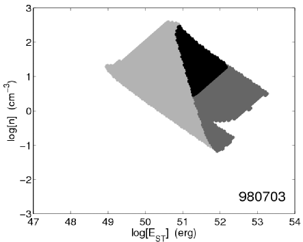
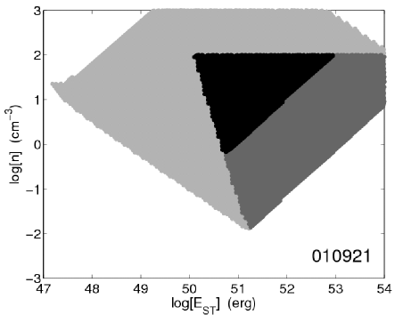
Figure 1.— Electron number density plotted against kinetic energy for two representative cases. The light gray regions indicate the phase-space that leads to a predicted flux density in agreement with the observed values. The medium gray regions encompass the subset of solutions that satisfy the condition $(E_{B}+E_{e})\lesssim E_{\rm ST}/2$. The black regions marks the subset of solutions that satisfy $\beta<1$ in the Sedov-Taylor framework. Left: Group A burst with a well-defined spectral peak. Right: Group B burst with a single frequency detection for which we use the additional limit that $n<100$ cm^-3. This figure highlights the significant advantage of measuring the spectral peak.

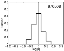
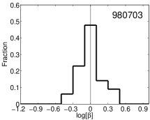
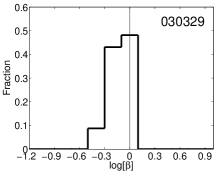
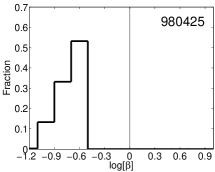
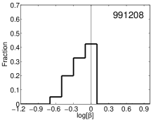
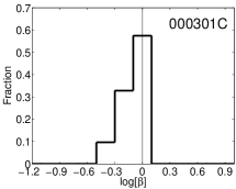
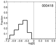
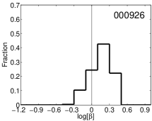
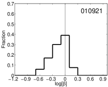
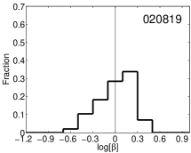
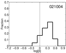
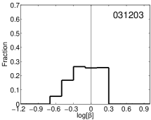
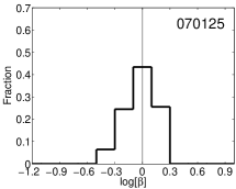
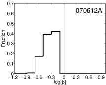
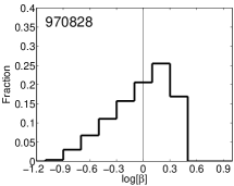
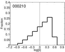
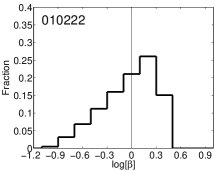
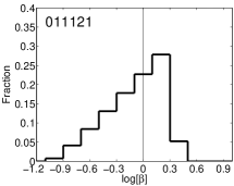
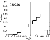
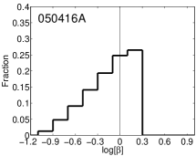
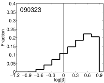
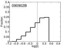
Figure 2.— Normalized histograms of inferred expansion velocity, $\beta\equiv v/c$, at the time of our observations. A value of $\lesssim 1$ (vertical lines) is required for self-consistency, and this is indeed the case for the bulk of the acceptable solutions. Note that the scales for the three groups are different.

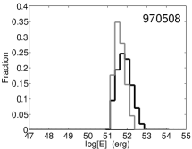
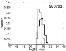
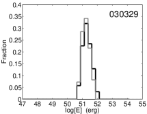
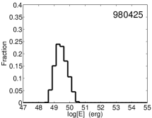
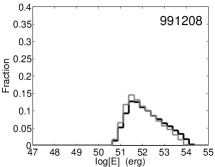
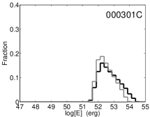
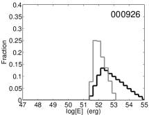
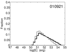
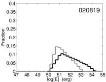
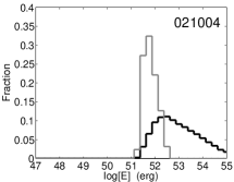
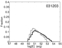
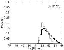
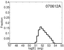
Figure 3.— Normalized histograms of GRB energies calculated using the Sedov-Taylor solution. The light gray histograms for some Group B bursts indicate the subset of solutions with a strict cut-off of $\beta<1$. GRBs 000926, 020819, and 021004 are rejected from our sample since the bulk of their solutions still lead to relativistic expansion.

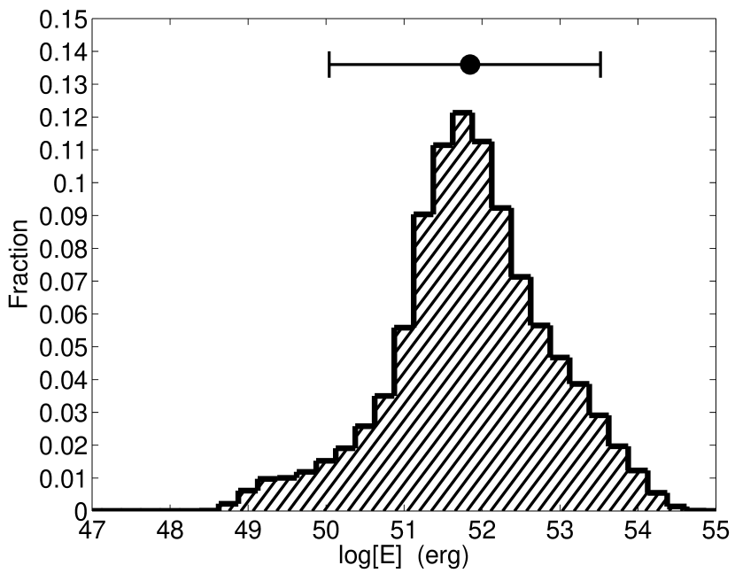
Figure 4.— Normalized distribution of GRB kinetic energies calculated using the Sedov-Taylor solution for the sample of 11 bursts with self-consistent solutions (Figure 3). The median and 90% confidence range are marked by a horizontal bar.

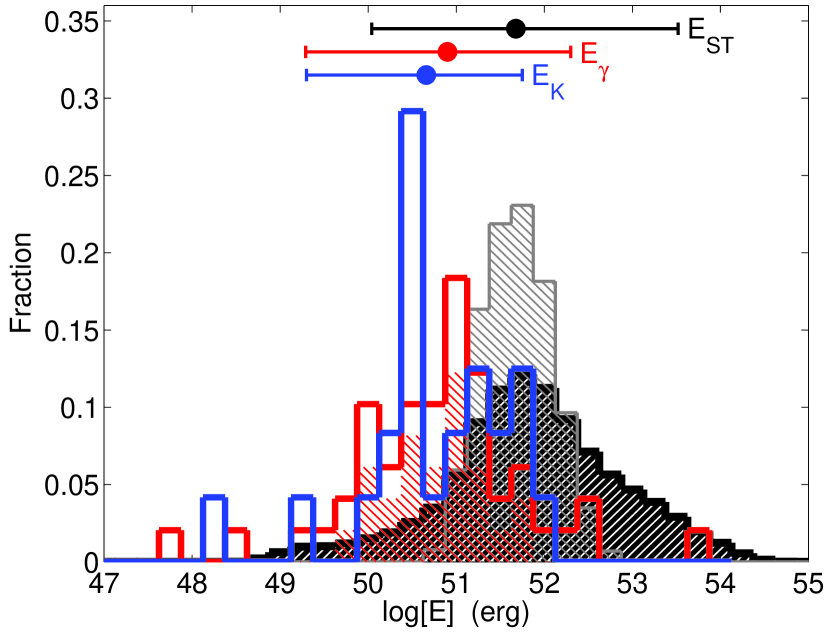
Figure 5.— Normalized distributions of GRB kinetic energies calculated using the Sedov-Taylor solution (black), and for the subset of 3 bursts in Group A (gray). Also shown for comparison are the distributions of beaming-corrected $\gamma$-ray energies (red: hatch = known $\theta_{j}$ values; open = $\theta_{j}$ lower or upper limits; Friedman & Bloom 2005) and beaming-corrected kinetic energies from broad-band early afterglow modeling (blue; Panaitescu & Kumar 2002; Berger et al. 2003b; Yost et al. 2003; Soderberg et al. 2004b, a, 2006; Cenko et al. 2010b, a). The median and $90\%$ confidence range for each energy component are marked by a horizontal bar. Our inferred median energy and $90\%$ confidence range are larger than the median of both $E_{\gamma}$ and $E_{K}$, but this is mainly due to the bursts in Group B for which the spectral peak is not measured. Future observations with the EVLA will lead to much tighter constraints (see gray histogram) for a larger sample.

References

- Berger et al. (2001) Berger, E., et al. 2001, ApJ, 556, 556
- Berger et al. (2002) Berger, E., et al. 2002, ApJ, 581, 981
- Berger et al. (2003a) Berger, E., Kulkarni, S. R., & Frail, D. A. 2003, ApJ, 590, 379
- Berger et al. (2004) Berger, E., Kulkarni, S. R., & Frail, D. A. 2004, ApJ, 612, 966
- Berger et al. (2003b) Berger, E., et al. 2003, Nature, 426, 154
- Berger et al. (2000) Berger, E., et al. 2000, ApJ, 545, 56
- Berger et al. (2005) Berger, E., et al. 2005, ApJ, 634, 501
- Bloom et al. (2003) Bloom, J. S., Frail, D. A., & Kulkarni, S. R. 2003, ApJ, 594, 674
- Cenko et al. (2010a) Cenko, S. B., et al. 2010a, arXiv:1004.2900
- Cenko et al. (2010b) Cenko, S. B., et al. 2010b, ApJ, 711, 641
- Chandra et al. (2008) Chandra, P., et al. 2008, ApJ, 683, 924
- Curran et al. (2008) Curran, P. A., Evans, P. A., de Pasquale, M., Page, M. J., & van der Horst, A. J. 2010, ApJ, 716, L135
- Djorgovski et al. (2001) Djorgovski, S. G., Frail, D. A., Kulkarni, S. R., Bloom, J. S., Odewahn, S. C., and Diercks, A. 2001, ApJ, 562, 654.
- Frail et al. (2003a) Frail, D. A., Kulkarni, S. R., Berger, E., & Wieringa, M. H. 2003a, AJ, 125, 2299
- Frail et al. (2001) Frail, D. A., et al. 2001, ApJ, 562, L55
- Frail et al. (2005) Frail, D. A., Soderberg, A. M., Kulkarni, S. R., Berger, E., Yost, S., Fox, D. W., & Harrison, F. A. 2005, ApJ, 619, 994
- Frail et al. (2000) Frail, D. A., Waxman, E., & Kulkarni, S. R. 2000, ApJ, 537, 191
- Frail et al. (2003b) Frail, D. A., et al. 2003b, ApJ, 590, 992
- Friedman & Bloom (2005) Friedman, A. S., & Bloom, J. S. 2005, ApJ, 627, 1
- Galama et al. (2003) Galama, T. J., Frail, D. A., Sari, R., Berger, E., Taylor, G. B., & Kulkarni, S. R. 2003, ApJ, 585, 899
- Harrison et al. (2001) Harrison, F. A., et al. 2001, ApJ, 559, 123
- Jakobsson et al. (2005) Jakobsson, P., et al. 2005, ApJ, 629, 45
- Jakobsson et al. (2006) Jakobsson, P., et al. 2006, A&A, 447, 897
- Kulkarni et al. (1998) Kulkarni, S. R., et al. 1998, Nature, 395, 663
- Liang et al. (2008) Liang, E., Racusin, J. L., Zhang, B., Zhang, B., & Burrows, D. N. 2008, ApJ, 675, 528
- Livio & Waxman (2000) Livio, M., & Waxman, E. 2000, ApJ, 538, 187
- Panaitescu & Kumar (2001) Panaitescu, A., & Kumar, P. 2001, ApJ, 560, L49
- Panaitescu & Kumar (2002) Panaitescu, A., & Kumar, P. 2002, ApJ, 571, 779
- Piro et al. (2002) Piro, L., et al. 2002, ApJ, 577, 680
- Price et al. (2002) Price, P. A., et al. 2002, ApJ, 573, 85
- Racusin et al. (2008) Racusin, J. L., et al. 2008, Nature, 455, 183
- Racusin et al. (2009) Racusin, J. L., et al. 2009, ApJ, 698, 43
- Rybicki & Lightman (1979) 1979, Radiative processes in astrophysics, ed. Rybicki, G. B. & Lightman, A. P.
- Soderberg et al. (2004a) Soderberg, A. M., et al. 2004a, ApJ, 606, 994
- Soderberg et al. (2004b) Soderberg, A. M., et al. 2004b, Nature, 430, 648
- Soderberg et al. (2006) Soderberg, A. M., et al. 2006, Nature, 442, 1014
- Soderberg et al. (2006) Soderberg, A. M., et al. 2007, ApJ, 661, 982
- Taylor et al. (2000) Taylor, G. B., Bloom, J. S., Frail, D. A., Kulkarni, S. R., Djorgovski, S. G., & Jacoby, B. A. 2000, ApJ, 537, L17
- Taylor et al. (2004) Taylor, G. B., Frail, D. A., Berger, E., & Kulkarni, S. R. 2004, ApJ, 609, L1
- van Eerten et al. (2010) van Eerten, H., Zhang, W., & MacFadyen, A. 2010, ApJ, 722, 235
- Yost et al. (2003) Yost, S. A., Harrison, F. A., Sari, R., & Frail, D. A. 2003, ApJ, 597, 459
- Zhang & MacFadyen (2009) Zhang, W., & MacFadyen, A. 2009, ApJ, 698, 1261