A low-memory algorithm for finding short product representations in finite groups

Abstract.

We describe a space-efficient algorithm for solving a generalization of the subset sum problem in a finite group $G$, using a Pollard-$\rho$ approach. Given an element $z$ and a sequence of elements $S$, our algorithm attempts to find a subsequence of $S$ whose product in $G$ is equal to $z$. For a random sequence $S$ of length $d\log_{2}n$, where $n=\#G$ and $d\geqslant 2$ is a constant, we find that its expected running time is $O(\sqrt{n}\log n)$ group operations (we give a rigorous proof for $d>4$), and it only needs to store $O(1)$ group elements. We consider applications to class groups of imaginary quadratic fields, and to finding isogenies between elliptic curves over a finite field.

1. Introduction

Let $S$ be a sequence of elements in a finite group $G$ of order $n$, written multiplicatively. We say that $S$ represents $G$ if every element of $G$ can be expressed as the (ordered) product of a subsequence of $S$. Ideally, we want $S$ to be short, say $k=d\log_{2}n$ for some constant $d$ known as the density of $S$.

In order for $S$ to represent $G$, we clearly require $d\geqslant 1$, and for sufficiently large $n$, any $d>1$ suffices. More precisely, Babai and Erdős [3] show that for all

$$k\geqslant\log_{2}n+\log_{2}\log n+2$$

there exists a sequence $S$ of length $k$ that represents $G$. Their proof is non-constructive, but, in the case that $G$ is abelian, Erdős and Rényi [10] show that a randomly chosen sequence of length

$$k=\log_{2}n+\log_{2}\log n+\omega_{n}$$

represents $G$ with probability approaching $1$ as $n\to\infty$, provided that $\omega_{n}\to\infty$. The randomness assumption is necessary, since it takes much larger values of $k$ to ensure that every sequence of length $k$ represents $G$, see [9, 33].

In related work, Impagliazzo and Naor prove that for a random sequence $S$ of density $d>1$, the distribution of subsequence products almost surely converges to the uniform distribution on $G$ as $n$ goes to infinity [15, Proposition 4.1]. This result allows us to bound the complexity of our algorithm for almost all $S$ with $d>4$.

Given a sequence $S$ that represents $G$ (or a large subset of $G$), we wish to find an explicit representation of a given group element $z$ as the product of a subsequence of $S$; we call this a short product representation of $z$. In the special case that $G$ is abelian and the elements of $S$ are distinct, this is the subset sum problem in a finite group. Variations of this problem and its decision version have long been of interest to many fields: complexity theory [17], cryptography [20], additive number theory [3], Cayley graph theory [2], and information theory [1], to name just a few.

As a computational framework, we work with a generic group $G$ whose elements are uniquely identified, and assume that all group operations are performed by a black box that can also provide random group elements; see [30, Chapter 1] for a formal model. Time complexity is measured by counting group operations (calls to the black box), and for space complexity we count the number of group elements that are simultaneously stored. In most practical applications, these metrics are within a polylogarithmic factor of the usual bit complexity.

Working in this model ensures that our algorithms apply to any finite group for which a suitable black box can be constructed. It also means that finding short product representations is provably hard. Indeed, the discrete logarithm problem in a cyclic group of prime order has a lower bound of $\Omega(\sqrt{n})$ in the generic group model [26], and is easily reduced to finding short product representations.

In the particular group $G=\mathbb{Z}/n\mathbb{Z}$, we note that finding short product representations is easier for non-generic algorithms: the problem can be lifted to $k$ subset sum problems in $\mathbb{Z}$, which for suitable inputs can be solved with a time and space complexity of $O(n^{0.3113})$ via [14], beating the $\Omega(\sqrt{n})$ generic lower bound noted above. This is not so surprising, since working with integers is often easier than working in generic groups; for instance, the discrete logarithm problem in $\mathbb{Z}$ corresponds to integer division and can be solved in quasi-linear time.

A standard technique for solving subset sum problems in generic groups uses a baby-step giant-step approach, which can also be used to find short product representations (Section 2.1). This typically involves $O(2^{k/2})$ group operations and storage for $O(2^{k/2})$ group elements. The space bound can be improved to $O(2^{k/4})$ via a method of Schroeppel and Shamir [24].

Here, we give a Pollard-$\rho$ type algorithm [21] for finding short product representations in a finite group (Section 2.2). It only needs to store $O(1)$ group elements, and, assuming $S$ is a random sequence of density $d>4$, we prove that its expected running time is $O(\sqrt{n}\log{n})$ group operations; alternatively, by dedicating $O(n^{\epsilon})$ space to precomputations, the time complexity can be reduced to $O(\sqrt{n})$ (Section 3).

We also consider two applications: representing elements of the class group of an imaginary quadratic number field as short products of prime ideals with small norm (Section 4.2), and finding an isogeny between two elliptic curves defined over a finite field (Section 4.3). For the latter, our method combines the advantages of [11] and [12] in that it requires little memory and finds an isogeny that can subsequently be evaluated in polynomial time.

In practice, our algorithm performs well so long as $d\geqslant 2$, and its low space complexity allows it to feasibly handle much larger problem instances than other generic methods (Section 5).

2. Algorithms

Let $S$ be a sequence of length $k$ in a finite group $G$ of order $n$, let $z$ be an element of $G$, and let $\mathcal{P}(S)$ denote the set of all subsequences of $S$. Our goal is to find a preimage of $z$ under the product map $\pi:\mathcal{P}(S)\to G$ that sends a subsequence of $S$ to the (ordered) product of its elements.

2.1. Baby-step giant-step

Let us first recall the baby-step giant-step method. We may express $S=AB$ as the concatenation of two subsequences of roughly equal length. For any sequence $y=(y_{1},\ldots,y_{m})$, let $\mu(y)=(y_{m}^{-1},\ldots,y_{1}^{-1})$, so that $\pi(y)$ and $\pi(\mu(y))$ are inverses in $G$. We then search for $x\in\mathcal{P}(A)$ (a baby step) and $y\in\mathcal{P}(B)$ (a giant step) which “collide” in the sense that $\pi(x)=\pi(z\mu(y))$, where $z\mu(y)$ denotes the sequence $(z,y_{m}^{-1},\ldots,y_{1}^{-1})$.

Baby-step giant-step Algorithm
Input: A finite sequence $S$ in a group $G$ and a target $z\in\pi(\mathcal{P}(S))$.
Output: A subsequence of $S$ whose product is $z$.
1. Express $S$ in the form $S=AB$ with $\#A\approx\#B$. 2. For each $x\in\mathcal{P}(A)$, store $(\pi(x),x)$ in a table indexed by $\pi(x)$. 3. For each $y\in\mathcal{P}(B)$: 4.     Lookup $\pi(z\mu(y))$ in the table computed in Step 2. 5.     If $\pi(z\mu(y))=\pi(x)$ is found then output $xy$, otherwise continue.

The table constructed in Step 2 is typically implemented as a hash table, so that the cost of the lookup in Step 4 is negligible. Elements of $\mathcal{P}(A)$ and $\mathcal{P}(B)$ may be compactly represented by bit-strings of length $\lceil k/2\rceil=O(\log n)$, which is approximately the size of a single group element. If these bit-strings are enumerated in a suitable order, each step can be derived from the previous step using $O(1)$ group operations. The algorithm then performs a total of $O(2^{k/2})$ group operations and has a space complexity of $O(2^{k/2})$ group elements. One can make a time-space trade off by varying the relative sizes of $A$ and $B$.

This algorithm has the virtue of determinism, but its complexity $O(n^{d/2})$ is exponential in the density $d$ (as well as $\log n$). For $d>1$, a randomized approach works better: select $\sqrt{n}$ baby steps $x\in\mathcal{P}(A)$ at random, then select random giant steps $y\in\mathcal{P}(B)$ until a collision $\pi(z\mu(y))=\pi(x)$ is found. Assuming that $\pi(x)$ and $\pi(z\mu(y))$ are uniformly distributed in $G$, we expect to use $\sqrt{n}$ giant steps. To reduce the cost of each step, one may partition $A$ and $B$ each into approximately $d$ subsequences $A_{i}$ and $B_{i}$ and precompute $\pi(x)$ for all $x\in\mathcal{P}(A_{i})$, and $\pi(\mu(y))$ for all $y\in\mathcal{P}(B_{i})$. This yields an expected running time of $O(\sqrt{n})$ group operations, using storage for $O(\sqrt{n})$ group elements, for any fixed $d$.

2.2. A low-memory algorithm

In order to use the Pollard-$\rho$ technique, we need a pseudo-random function $\phi$ on the disjoint union $\mathcal{C}=\mathcal{A}\sqcup\mathcal{B}$, where $\mathcal{A}=\mathcal{P}(A)$ and $\mathcal{B}$ is the set $\{z\mu(y):y\in\mathcal{P}(B)\}$. This map $\phi$ is required to preserve collisions, meaning that $\pi(x)=\pi(y)$ implies $\pi(\phi(x))=\pi(\phi(y))$. Given a hash function $\eta:G\to\mathcal{C}$, we may construct such a map as $\phi=\eta\circ\pi$. Under suitable assumptions (see Section 3), the Pollard-$\rho$ method can then be applied.

Pollard-$\rho$ Algorithm
Input: A finite sequence $S$ in a group $G$ and a target $z\in\pi(\mathcal{P}(S))$.
Output: A subsequence of $S$ whose product is $z$.
1. Pick a random element $w\in\mathcal{C}$ and a hash function $\eta:G\to\mathcal{C}$. 2. Find the least $i>0$ and $j\geqslant 0$ such that $\phi^{(i+j)}(w)=\phi^{(j)}(w)$. 3. If $j=0$ then return to Step 1. 4. Let $s=\phi^{(i+j-1)}(w)$ and let $t=\phi^{(j-1)}(w)$. 5. If $\pi(s)\neq\pi(t)$ then return to Step 1. 6. If $s\in\mathcal{A}$ and $t=z\mu(y)\in\mathcal{B}$ then output $sy$ and terminate. 7. If $t\in\mathcal{A}$ and $s=z\mu(y)\in\mathcal{B}$ then output $ty$ and terminate. 8. Return to Step 1.

Step 2 can be implemented with Floyd’s algorithm [18, Exercise 3.1.6] using storage for just two elements of $\mathcal{C}$, which fits in the memory space of $O(1)$ group elements. More sophisticated collision-detection techniques can reduce the number of evaluations of $\phi$ while still storing $O(1)$ elements, see [7, 25, 31]. We prefer the method of distinguished points, which facilitates a parallel implementation [32].

2.3. Toy example

Let $G=(\mathbb{Z}/n\mathbb{Z},+)$ and define $S$ as the concatenation of the sequences $A=(3^{i})$ and $B=(5^{i})$ for $i\in\{1,\ldots,k/2\}$. We put $n=127$ and $k=12$, implying $d\approx 1.7$. With $\mathcal{C}=\mathcal{A}\sqcup\mathcal{B}$ as above, we define $\eta:G\to\mathcal{C}$ via

$$x\longmapsto\left\{\begin{array}[]{cl}(A_{i})_{\{i:b_{i}=1\}}&\text{when }b_{0}=1\\ z\mu\left((B_{i})_{\{i:b_{i}=1\}}\right)&\text{when }b_{0}=0\end{array}\right.$$

where $\sum_{i=0}^{k/2}b_{i}2^{i}$ is the binary representation of $96x\bmod n$.

Starting from $w=(2,-5^{6},-5^{3},-5^{2},-5)$, the algorithm finds $i=4$ and $j=6$:

The two preimages of $(3^{2},3^{4})$ yield the short product representation

$$2\equiv 3+3^{2}+3^{3}+3^{5}+5+5^{2}+5^{4}+5^{5}+5^{6}\bmod 127.$$

3. Analysis

The Pollard-$\rho$ approach is motivated by the following observation: if $\phi:X\to X$ is a random function on a set $X$ of cardinality $n$, then the expected size of the orbit of any $x\in X$ under the action of $\phi$ is $\sqrt{\pi n/2}$ (see [28] for a rigorous proof). In our setting, $X$ is the set $\mathcal{C}$ and $\phi=\eta\circ\pi$. Alternatively, since $\phi$ preserves collisions, we may regard $X$ as the set $\pi(\mathcal{C})\subset G$ and use $\varphi=\pi\circ\eta$. We shall take the latter view, since it simplifies our analysis.

Typically the function $\varphi$ is not truly random, but under a suitable set of assumptions it may behave so. To rigorously analyze the complexity of our algorithm, we fix a real number $d>4$ and assume that:

1. the hash function $\eta:G\to\mathcal{C}$ is a random oracle;

2. $S$ is a random sequence of density $d$.

For any finite set $U$, let $\mathbb{U}_{U}$ denote the uniform distribution on $U$, which assigns to each subset $X$ of $U$ the value $\#X/\#U$. For any function $f:U\to V$, let $f_{*}\mathbb{U}_{U}$ denote the pushforward distribution by $f$ of $\mathbb{U}_{U}$, which assigns to each subset $Y$ of $V$ the value

$$f_{*}\mathbb{U}_{U}(Y)=\frac{\#\{u\in U:f(u)\in Y\}}{\#U}.$$

Assumption (2) implies that $A$ and $B$ are both random sequences with density greater than $2$. By [15, Proposition 4.1], this implies that

$$\operatorname{Prob}_{A}\left[\left\|\pi_{*}\mathbb{U}_{\mathcal{A}}-\mathbb{U}_{G}\right\|\geqslant n^{-c}\right]\leqslant n^{-c},$$

where $c=(d-2)/4>1/2$, and the variation distance $\|\sigma-\tau\|$ between two distributions $\sigma$ and $\tau$ on $G$ is defined as the maximum value of $|\sigma(H)-\tau(H)|$ over all subsets $H$ of $G$. Similarly, we have

$$\operatorname{Prob}_{B}\left[\left\|\pi_{*}\mathbb{U}_{\mathcal{B}}-\mathbb{U}_{G}\right\|\geqslant n^{-c}\right]\leqslant n^{-c}.$$

From now on we assume that $S$ is fixed and that $\pi_{*}\mathbb{U}_{C}$ is within variation distance $2n^{-c}$ of the uniform distribution on $G$; by the argument above, this happens with probability at least $1-2n^{-c}$. Recall that a random oracle $\eta:G\to\mathcal{C}$ is a random function drawn uniformly from $\mathcal{C}^{G}$, that is, each value $\eta(x)$ is drawn uniformly and independently from $\mathcal{C}$. Thus, for any $g\in G$, the distribution of $\pi(\eta(g))$ is $\pi_{*}\mathbb{U}_{C}$. It is then easy to verify that

$$\left\|(\eta\mapsto\pi\circ\eta)_{*}\mathbb{U}_{\mathcal{C}^{G}}-\mathbb{U}_{G^{G}}\right\|\leqslant 2n^{-c}.$$

In other words, for a random oracle $\eta$, the function $\varphi=\pi\circ\eta$ is very close to being a random oracle (from $G$ to $G$) itself.

Since $c>1/2$, we obtain, as in [21], an $O(\sqrt{n})$ bound on the expectation of the least positive integer $i+j$ for which $\varphi^{(i+j)}(g)=\varphi^{(j)}(g)$, for any $g=\pi(w)\in G$. For $d>2$, the probability that $\pi(s)\neq\pi(t)$ in Step 5 is $o(1)$, since $\mathcal{C}$ is then larger than $G$ and collisions in the map $\varphi$ (and $\phi$) are more likely to be caused by collisions in $\pi$ than collisions in $\eta$. Having reached Step 6, we obtain a short product representation of $z$ with probability $1/2$, since by results of [15] the value of $\pi(x)$ is independent of whether $x\in\mathcal{A}$ or $x\in\mathcal{B}$. The expected running time is thus $O(k\sqrt{n})=O(\sqrt{n}\log n)$ group operations, and, as noted in Section 2.2, the space complexity is $O(1)$ group elements. We summarize our analysis with the following proposition.

Proposition.

Let $S$ be a random sequence of constant density $d>4$ and let $\eta:G\to\mathcal{C}$ be a random oracle. Then our Pollard-$\rho$ algorithm uses $O(\sqrt{n}\log n)$ expected group operations and storage for $O(1)$ group elements.

As in Section 2.1, to speed up the evaluation of the product map $\pi$, one may partition $A$ and $B$ into subsequences $A_{i}$ and $B_{i}$ of length $m$ and precompute $\pi(\mathcal{P}(A_{i}))$ and $\pi(\mu(\mathcal{P}(B_{i}))$. This requires storage for $O(k2^{m}/m)$ group elements and speeds up subsequent evaluations of $\pi$ by a factor of $m$. If we let $m=\epsilon\log_{2}n$, for any $\epsilon>0$, we obtain the following corollary.

Corollary.

Under the hypotheses of the proposition above, our Pollard-$\rho$ algorithm can be implemented to run in expected time $O(\sqrt{n})$ using $O(n^{\epsilon})$ space.

In our analysis above, we use a random $S$ random with $d>4$ to prove that products of random elements of $\mathcal{A}$ and $\mathcal{B}$ are quasi-uniformly distributed in $G$. If we directly assume that both $\pi_{*}\mathbb{U}_{\mathcal{A}}$ and $\pi_{*}\mathbb{U}_{\mathcal{B}}$ are quasi-uniformly distributed, our analysis applies to all $d\geqslant 2$, and in practice we find this to be the case. However, we note that this does not apply to $d<2$, for which we expect a running time of $O(n^{(4-d)/4}\log n)$, as discussed in Section 5.

4. Applications

As a first application, let us consider the case where $G$ is the ideal class group of an order $\mathcal{O}$ in an imaginary quadratic field. We may assume

$$\mathcal{O}=\mathbb{Z}+\frac{D+\sqrt{D}}{2}\mathbb{Z},$$

where the discriminant $D$ is a negative integer congruent to $0$ or $1$ modulo $4$. Modulo principal ideals, the invertible ideals of $\mathcal{O}$ form a finite abelian group $\operatorname{cl}(\mathcal{O})$ of cardinality $h$. The class number $h$ varies with $D$, but is on average proportional to $\sqrt{|D|}$ (more precisely, $\log h\sim\frac{1}{2}\log|D|$ as $D\to-\infty$, by Siegel’s theorem [27]). Computationally, invertible $\mathcal{O}$-ideals can be represented as binary quadratic forms, allowing group operations in $\operatorname{cl}(\mathcal{O})$ to be computed in time $O(\log^{1+\epsilon}|D|)$, via [22].

4.1. Prime ideals

Let $\ell_{i}$ denote the $i$^th largest prime number for which there exists an invertible $\mathcal{O}$-ideal of norm $\ell_{i}$ and let $\alpha_{i}$ denote the unique such ideal that has nonnegative trace. For each positive integer $k$, let $S_{k}$ denote the sequence of (not necessarily distinct) ideal classes

$$S_{k}=([\alpha_{1}],[\alpha_{2}],\ldots,[\alpha_{k}]).$$

For algorithms that work with ideal class groups, $S_{k}$ is commonly used as a set of generators for $\operatorname{cl}(\mathcal{O})$, and in practice $k$ can be made quite small, conjecturally $O(\log h)$. Proving such a claim is believed to be very difficult, but under the generalized Riemann hypothesis (GRH), Bach obtains the following result [4].

Theorem (Bach).

Assume the GRH. If $D$ is a fundamental discriminant and $\ell_{k+1}>6\log^{2}|D|$, then the set $S_{k}$ generates $\operatorname{cl}(\mathcal{O})$.

Unfortunately, this says nothing about short product representations in $\operatorname{cl}(\mathcal{O})$. Recently, a special case of [16, Corollary 1.3] was considered in [8, Theorem 2.1] which still assumes the GRH but is more suited to our short product representation setting. Nevertheless, for our purpose here, we make the following stronger conjecture.

Conjecture.

For every $d_{0}>1$ there exist constants $c>0$ and $D_{0}<0$ such that if $D\leqslant D_{0}$ and $S_{k}$ has density $d\geqslant d_{0}$ then

1. $\pi(\mathcal{P}(S_{k}))=G$, that is, $S_{k}$ represents $G$;

2. $\left\|\pi_{*}\mathbb{U}_{\mathcal{P}(S_{k})}-\mathbb{U}_{G}\right\|<h^{-c}$;

where $G$ is the ideal class group $\operatorname{cl}(\mathcal{O})$ and $h$ is its cardinality.

In essence, these are heuristic analogs to the results of Erdős and Rényi, and of Impagliazzo and Naor, respectively, suggesting that the distribution of the classes $[\alpha_{i}]$ resembles that of random elements uniformly drawn from $\operatorname{cl}(\mathcal{O})$. Note that (1), although seemingly weaker, is only implied by (2) when $c>1$.

Empirically, (1) is easily checked: for $d_{0}=2$ we have verified it using $D_{0}=-3$ for every imaginary quadratic order with discriminant $D\geqslant-10^{8}$, and for $10^{4}$ randomly chosen orders with $D$ logarithmically distributed over the interval $[-10^{16},-10^{8}]$ (see Figure 1). Although harder to test, (2) is more natural in our context, and practical computations support it as well. Even though we see no way to prove this conjecture, we assume its veracity as a useful heuristic.

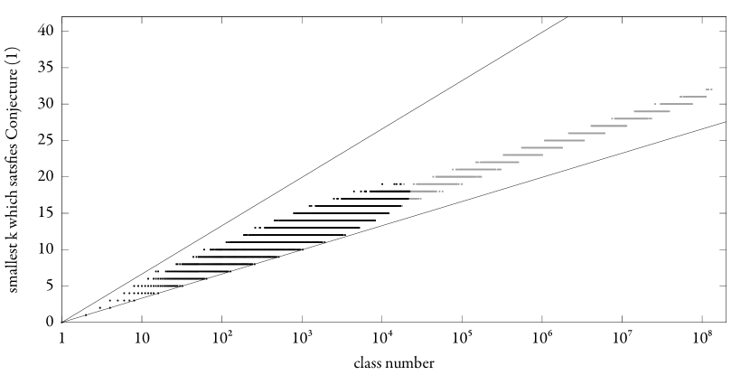
Figure 1. Dots plot the minimal $k$ such that $S_{k}$ satisfies conjecture (1); gray dots for all discriminants $D\geqslant-10^{8}$ and black dots for ten thousand $D$ drawn at random according to a logarithmic distribution. The lines represent $k=d\log_{2}h$ for $d=1,2$.

4.2. Short relations

In [13], Hafner and McCurley give a subexponential algorithm to find representatives of the form $\prod\alpha_{i}^{e_{i}}$ for arbitrary ideal classes of imaginary quadratic orders; the ideals $\alpha_{i}$ have subexponential norms, but the exponents $e_{i}$ can be as large as the class number $h$.

Asking for small exponents $e_{i}\in\{0,1\}$ means, in our terminology, writing elements $z\in G$ as short product representations on $S_{k}=([\alpha_{i}])$. Under the conjecture above, this can be achieved by our low-memory algorithm in $O(|D|^{1/4+\epsilon})$ expected time, using $k=O(\log h)$ ideals $\alpha_{i}$.

We can even combine these approaches. If the target element $z$ is represented by an ideal of small norm, say $z=[\alpha_{k+1}]$, we get what we call a short relation for $\operatorname{cl}(\mathcal{O})$. Conjecture (1) implies not only that the map that sends each vector $(e_{1},\ldots,e_{k+1})\in\mathbb{Z}^{k+1}$ to the class of the ideal $\prod\alpha_{i}^{e_{i}}$ is surjective, but also that there exists a set of short relations generating its kernel lattice $\Lambda$. This gives a much better upper bound on the diameter of $\Lambda$ than was used by Hafner and McCurley, and their algorithm can be adapted to make use of this new bound and find, in subexponential time, representatives $\prod\alpha_{i}^{e_{i}}$ with ideals $\alpha_{i}$ of subexponential norm and exponents $e_{i}$ bounded by $O(\log|D|)$. See [5] for details, or [8] for an equivalent construction.

4.3. Short isogenies

Now let us consider the problem of finding an isogeny between two ordinary elliptic curves $E_{1}$ and $E_{2}$ defined over a finite field $\mathbb{F}_{q}$. This problem is of particular interest to cryptography because the discrete logarithm problem can then be transported from $E_{1}$ to $E_{2}$. An isogeny between curves $E_{1}$ and $E_{2}$ exists precisely when $E_{1}$ and $E_{2}$ lie in the same isogeny class. By a theorem of Tate, this occurs if and only if $\#E_{1}(\mathbb{F}_{q})=\#E_{2}(\mathbb{F}_{q})$, which can be determined in polynomial time using Schoof’s algorithm [23].

The isogeny class of $E_{1}$ and $E_{2}$ can be partitioned according to the endomorphism rings of the curves it contains, each of which is isomorphic to an order $\mathcal{O}$ in an imaginary quadratic number field. Identifying isomorphic curves with their $j$-invariant, for each order $\mathcal{O}$ we define

$$\operatorname{Ell}(\mathcal{O})=\left\{j(E):\operatorname{End}(E)\cong\mathcal{O}\right\},$$

where $E$ denotes an elliptic curve defined over $\mathbb{F}_{q}$. The set $\operatorname{Ell}(\mathcal{O})$ to which a given curve belongs can be determined in subexponential time, under heuristic assumptions [6]. An isogeny from $E_{1}$ to $E_{2}$ can always be decomposed into two isogenies, one that is essentially determined by $\operatorname{End}(E_{1})$ and $\operatorname{End}(E_{2})$ (and can be made completely explicit but may be difficult to compute), and another connecting curves that lie in the same set $\operatorname{Ell}(\mathcal{O})$. We shall thus restrict ourselves to the problem of finding an isogeny between two elements of $\operatorname{Ell}(\mathcal{O})$.

The theory of complex multiplication states that $\operatorname{Ell}(\mathcal{O})$ is a principal homogeneous space (a torsor) for the class group $\operatorname{cl}(\mathcal{O})$: each ideal $\alpha$ acts on $\operatorname{Ell}(\mathcal{O})$ via an isogeny of degree $\operatorname{N}(\alpha)$, and this action factors through the class group. We may then identify each ideal class $[\alpha]$ with the image $[\alpha]j(E_{i})$ of its action on $j(E_{i})$. This allows us to effectively work in the group $\operatorname{cl}(\mathcal{O})$ when computing isogenies from $E_{i}$.

Galbraith addressed the search for an isogeny $E_{1}\to E_{2}$ using a baby-step giant-step approach in [11]; a low-memory variant was later given in [12] which produces an exponentially long chain of low-degree isogenies. From that, a linearly long chain of isogenies of subexponential degree may be derived by smoothing the corresponding ideal in $\operatorname{cl}(\mathcal{O})$ using variants of the method of Hafner and McCurley (for instance, those mentioned in Section 4.2); alternatively, our low-memory algorithm can be used to derive a chain of low-degree isogenies with length linear in $\log|D|$ (assuming our conjecture), and we believe this is the most practical approach. However, let us describe how our method applies naturally to the torsor $\operatorname{Ell}(\mathcal{O})$, and directly finds a short chain of low-degree isogenies from $E_{1}$ to $E_{2}$ using very little memory.

Let $S_{k}=AB$ be such that conjecture (1) holds, where $A$ and $B$ are roughly equal in size, and define $\mathcal{C}=\mathcal{A}\sqcup\mathcal{B}$ where $\mathcal{A}=\mathcal{P}(A)$ and $\mathcal{B}=\mu(\mathcal{P}(B))$. We view each element of $\mathcal{A}$ as a short chain of isogenies of small prime degree $\ell_{i}=\operatorname{N}(\alpha_{i})$ that originates at $E_{1}$; similarly, we view elements of $\mathcal{B}$ as chains of isogenies originating at $E_{2}$. Now let $\pi:\mathcal{C}\to\operatorname{Ell}(\mathcal{O})$ be the map that sends $x\in\mathcal{A}$ (resp. $x\in\mathcal{B}$) to the element of $\operatorname{Ell}(\mathcal{O})$ that is the codomain of the isogeny chain defined by $x$ and originating at $E_{1}$ (resp. $E_{2}$). It suffices to find a collision between an element of $\mathcal{A}$ and an element of $\mathcal{B}$ under the map $\pi$: this yields an isogeny chain from $E_{1}$ and an isogeny chain from $E_{2}$ that have the same codomain. Composing the first with the dual of the second gives an isogeny from $E_{1}$ to $E_{2}$.

The iteration function $\phi$ on $\mathcal{C}$ can now be defined as the composition $\eta\circ\pi$ where $\eta$ is a map from $\operatorname{Ell}(\mathcal{O})$ to $\mathcal{C}$ that behaves like a random oracle. Using this formalism, our Pollard-$\rho$ algorithm can be applied directly, and under the conjecture it finds an isogeny in time $O(h^{1/2+\epsilon})$. In terms of space, it only needs to store $O(1)$ elements of $\operatorname{cl}(\mathcal{O})$ and $\operatorname{Ell}(\mathcal{O})$, which is $O(\log q)$ bits. However, in order to compute isogenies, modular polynomials $\Phi_{\ell}(X,Y)$ might be used, each of which requires $O(\ell^{3}\log\ell)$ bits. If we heuristically assume that $\ell_{k}=O(k\log k)=O(\log h\log\log h)$, the overall space complexity is then bounded by $O(\log^{3+\epsilon}h)=O(\log^{3+\epsilon}q)$ bits, which is polynomial in $\log q$. This can be improved to $O(\log^{2+\epsilon}q)$ bits by using the algorithm of [29] to directly compute $\Phi_{\ell}(j(E),Y)$ in a space-efficient manner.

5. Computations

To test our generic low-memory algorithm for finding short product representations in a practical setting, we implemented black-boxes for three types of finite groups:

1. $G=E(\mathbb{F}_{p})$, the elliptic curve $E:y^{2}=x^{3}+x+1$ over a finite field $\mathbb{F}_{p}$.

2. $G=\operatorname{cl}(\mathcal{O})$, where $\mathcal{O}$ is an order in an imaginary quadratic field.

3. $G=\operatorname{GL}(2,\mathbb{F}_{p})$, the group of invertible $2\times 2$ matrices over $\mathbb{F}_{p}$.

To simplify the implementation, we restricted to cases where $\mathbb{F}_{p}$ is a prime field. The groups $E(\mathbb{F}_{p})$ are abelian groups, either cyclic or the product of two cyclic groups. The groups $\operatorname{cl}(\mathcal{O})$ are also abelian, but may be highly non-cyclic (we specifically chose some examples with large $2$-rank), while the groups $\operatorname{GL}(2,\mathbb{F}_{p})$ are non-abelian.

For the groups $E(\mathbb{F}_{p})$, we used the sequence of points $S=(P_{1},\ldots,P_{k})$ with $P_{i}=(x_{i},y_{i})$, where $x_{i}$ is the $i$^th smallest positive integer for which $x_{i}^{3}+x_{i}+1$ is a quadratic residue $y_{i}^{2}$ modulo $p$ with $y_{i}\leqslant(p-1)/2$; our target $z$ was the point $P_{k+1}$. For the groups $\operatorname{cl}(\mathcal{O})$, we used the sequence $S_{k}$ defined in Section 4.1 with $z=[\alpha_{k+1}]$. For the groups $\operatorname{GL}(2,\mathbb{F}_{p})$, we simply chose a sequence $S$ of length $k$ and a target element $z$ at random.

Table 1 lists performance data obtained by applying our Pollard-$\rho$ algorithm to various groups $G$ and sequences $S$ of densities $d=k/\log_{2}n$ ranging from just under $2$ to slightly more than $4$. Each row compares expected values with actual results that are averages over at least $10^{3}$ runs.

The parameter $c$ counts the number of collisions $\phi^{(i+j)}(w)=\phi^{(j)}(w)$ that were needed for a run of the algorithm to obtain a short product representation. Typically $c$ is greater than $1$ because not every collision yields a short product representation. The parameter $\rho_{\text{tot}}$ is the sum of $\rho=i+j$ over the $c$ collisions required, and represents a lower bound on the number of times the map $\phi$ was evaluated. With efficient collision detection, the actual number is very close to $\rho_{\text{tot}}$ (using the method of distinguished points we were able to stay within $1\%$).

					expected			observed
$G$	$\log_{2}n$	$k$	$d$		$c$	$\rho_{\text{tot}}$		$c$	$\rho_{\text{tot}}$
$E/\mathbb{F}_{2^{20}+7}$	20.00	40	2.00		3.00	3144		3.00	3162
		60	3.00		2.00	2568		2.01	2581
		80	4.00		2.00	2567		2.01	2565
$E/\mathbb{F}_{2^{24}+43}$	24.00	48	2.00		3.00	12577		3.02	12790
		72	3.00		2.00	10269		2.03	10381
		96	4.00		2.00	10268		2.00	10257
$E/\mathbb{F}_{2^{28}+3}$	28.00	56	2.00		3.00	50300		2.95	49371
		84	3.00		2.00	41070		2.02	41837
		112	4.00		2.00	41069		1.98	40508
$E/\mathbb{F}_{2^{32}+15}$	32.00	64	2.00		3.00	201196		3.06	205228
		96	3.00		2.00	164276		1.96	160626
		128	4.00		2.00	164276		2.04	169595
$E/\mathbb{F}_{2^{36}+31}$	36.00	72	2.00		3.00	804776		2.95	796781
		108	3.00		2.00	657097		2.00	655846
		144	4.00		2.00	657097		1.98	657097
$E/\mathbb{F}_{2^{40}+15}$	40.00	80	2.00		3.00	3219106		2.90	3120102
		120	3.00		2.00	2628390		1.97	2604591
		160	4.00		2.00	2628390		2.06	2682827
$\operatorname{cl}(1-2^{40})$	19.07	40	2.10		2.52	2088		2.44	2082
		60	3.15		2.00	1859		2.02	1845
		80	4.20		2.00	1858		2.01	1863
$\operatorname{cl}(1-2^{48})$	23.66	48	2.03		2.79	10800		2.75	10662
		72	3.04		2.00	9140		1.97	8938
		96	4.06		2.00	9140		1.99	9079
$\operatorname{cl}(1-2^{56})$	27.54	56	2.03		2.73	40976		2.69	40512
		84	3.05		2.00	35076		2.06	36756
		112	4.07		2.00	35076		1.98	35342
$\operatorname{cl}(1-2^{64})$	30.91	64	2.07		2.47	125233		2.59	131651
		96	3.11		2.00	112671		1.98	111706
		128	4.14		2.00	112671		1.99	111187
$\operatorname{cl}(1-2^{72})$	35.38	72	2.04		2.65	609616		2.60	598222
		108	3.05		2.00	529634		2.00	534639
		144	4.07		2.00	529634		2.00	532560
$\operatorname{cl}(1-2^{80})$	39.59	80	2.02		2.76	2680464		2.80	2793750
		120	3.03		2.00	2283831		2.01	2318165
		160	4.04		2.00	2283831		2.04	2364724
$\operatorname{GL}(2,\mathbb{F}_{37})$	20.80	42	2.02		2.87	4053		2.84	4063
		62	2.98		2.00	3384		1.99	3358
		84	4.04		2.00	3384		1.97	3388
$\operatorname{GL}(2,\mathbb{F}_{67})$	24.24	48	1.98		3.18	14087		3.08	13804
		72	2.97		2.00	11168		2.10	11590
		96	3.96		2.00	11167		2.01	11167
$\operatorname{GL}(2,\mathbb{F}_{131})$	28.12	56	1.99		3.09	53251		3.03	52070
		84	2.99		2.00	42851		1.94	42019
		112	3.98		2.00	42851		1.98	42146
$\operatorname{GL}(2,\mathbb{F}_{257})$	32.02	64	2.00		3.01	202769		3.03	204827
		96	3.00		2.00	165237		2.02	165742
		128	4.00		2.00	165237		2.00	165619
$\operatorname{GL}(2,\mathbb{F}_{511})$	36.10	72	1.99		3.07	842191		3.18	886141
		108	2.99		2.00	679748		1.97	668416
		144	3.99		2.00	679747		2.04	703877
$\operatorname{GL}(2,\mathbb{F}_{1031})$	40.04	80	2.00		3.03	3276128		2.99	3243562
		120	3.00		2.00	2663155		2.02	2677122
		160	4.00		2.00	2663154		2.08	2708512

Table 1. Comparison of expected vs. observed values on various groups.

The expected values of $c$ and $\rho_{\text{tot}}$ listed in Table 1 were computed under the heuristic assumption that $\eta:G\to\mathcal{C}$ and $\pi:\mathcal{C}\to G$ are both random functions. This implies that while iterating $\phi$ we are effectively performing simultaneous independent random walks on $G$ and $\mathcal{C}$. Let $X$ and $Y$ be independent random variables for the number of steps these walks take before reaching a collision, respectively. The probability that $\pi(s)=\pi(t)$ in Step 5 is $P(X\leqslant Y)$, and the algorithm then proceeds to find a short product representation with probability $1/2$.

Using the probability density $u\exp(-u^{2}/2)du$ of $X/\sqrt{\#G}$ and $Y/\sqrt{\#\mathcal{C}}$, we find

$$\operatorname{\mathbf{E}}[c]=2/{P(X\leqslant Y)}=2(1+r),$$

where $r=\#G/\#\mathcal{C}$. One may also compute

$$\operatorname{\mathbf{E}}[\rho_{\text{tot}}]=\operatorname{\mathbf{E}}[c]\operatorname{\mathbf{E}}[\min(X,Y)]=\sqrt{2\pi n(1+r)}.$$

For $d>2$, we have $r\approx 0$ for large $n$, so that $\operatorname{\mathbf{E}}[c]\approx 2$ and $\operatorname{\mathbf{E}}[\rho_{\text{tot}}]\approx\sqrt{2\pi n}$. For $d=2$, we have $\operatorname{\mathbf{E}}[c]=3$ and $\operatorname{\mathbf{E}}[\rho_{\text{tot}}]=\sqrt{3\pi n}$ (when $k$ is even). For $d<2$, the value of $\operatorname{\mathbf{E}}[c]$ increases with $n$ and we have $\operatorname{\mathbf{E}}[\rho_{\text{tot}}]=O(n^{(4-d)/4})$.

In addition to the tests summarized in Table 1, we applied our low memory algorithm to some larger problems that would be quite difficult to address with the baby-step giant-step method. Our first large test used $G=E(\mathbb{F}_{p})$ with $p=2^{80}+13$, which is a cyclic group of order $n=p+1+1475321552477$, and the sequence $S=(P_{1},\ldots,P_{k})$ with points $P_{i}$ defined as above with $k=200$, which gives $d\approx 2.5$. Our target element was $z=P_{201}$ with $x$-coordinate $391$. The computation was run in parallel on $32$ cores (3.0 GHz AMD Phenom II), using the distinguished points method. The second collision yielded a short product representation after evaluating the map $\phi$ a total of $1480862431620\approx 1.35\sqrt{n}$ times.

After precomputing $655360$ partial products (as discussed in Section 3), each evaluation of $\phi$ used $5$ group operations, compared to an average of $50$ without precomputation, and this required just $10$ megabytes of memory. The entire computation used approximately $140$ days of CPU time, and the elapsed time was about $4$ days. We obtained a short product representation for $z$ as the sum of $67$ points $P_{i}$ with $x$-coordinates less than $391$. In hexadecimal notation, the bit-string that identifies the corresponding subsequence of $S$ is:

542ab7d1f505bdaccdbeb6c2e92180d5f38a20493d60f031c1

Our second large test used the group $G=\operatorname{cl}(1-2^{160})$, which is isomorphic to

$$(\mathbb{Z}/2\mathbb{Z})^{8}\times\mathbb{Z}/4\mathbb{Z}\times\mathbb{Z}/8\mathbb{Z}\times\mathbb{Z}/80894875660895214584\mathbb{Z},$$

see [30, Table B.4]. We used the sequence $S_{k}$ with $k=200$, and chose the target $z=[\alpha_{201}]$ with $\operatorname{N}(\alpha_{201})=2671$. We ran the computation in parallel on $48$ cores, and needed $3$ collisions to obtain a short product representation, which involved a total of $2856153808020\approx 3.51\sqrt{n}$ evaluations of $\phi$. As in the first test, we precomputed $655360$ partial products so that each evaluation of $\phi$ used $5$ group operations. Approximately $900$ days of CPU time were used (the group operation in $\operatorname{cl}(D)$ is slower than in the group $E(\mathbb{F}_{p})$ used in our first example). We obtained a representative for the ideal class $z$ as the product of $106$ ideals with prime norms less than $2671$. The bit-string that encodes the corresponding subsequence of $S_{k}$ is:

5cf854598d6059f607c6f17b8fb56314e87314bee7df9164cd

References

- [1] Noga Alon, Amnon Barak, and Udi Manber. On disseminating information reliably without broadcasting. In Radu Popescu-Zeletin, Gerard Le Lann, and Kane H. Kim, editors, Proceedings of the 7th International Conference on Distributed Computing Systems, pages 74–81. IEEE Computer Society Press, 1987.
- [2] Noga Alon and Vitali D. Milman. , isoperimetric inequalities for graphs, and superconcentrators. Journal of Combinatorial Theory, Series B, 38:73–88, 1985.
- [3] László Babai and Paul Erdős. Representation of group elements as short products. North-Holland Mathematics Studies, 60:27–30, 1982.
- [4] Eric Bach. Explicit bounds for primality testing and related problems. Mathematics of Computation, 55(191):355–380, 1990.
- [5] Gaetan Bisson. Computing endomorphism rings of elliptic curves under the GRH, 2010. In preparation.
- [6] Gaetan Bisson and Andrew V. Sutherland. Computing the endomorphism ring of an ordinary elliptic curve over a finite field. Journal of Number Theory, Special Issue on Elliptic Curve Cryptography, 2009. To appear.
- [7] Richard P. Brent. An improved Monte Carlo factorization algorithm. BIT Numerical Mathematics, 20:176–184, 1980.
- [8] Andrew M. Childs, David Jao, and Vladimir Soukharev. Constructing elliptic curve isogenies in quantum subexponential time, 2010. Preprint available at http://arxiv.org/abs/1012.4019.
- [9] Roger B. Eggleton and Paul Erdős. Two combinatorial problems in group theory. Acta Arithmetica, 28:247–254, 1975.
- [10] Paul Erdős and Alfréd Rényi. Probabilistic methods in group theory. Journal d’Analyse Mathématique, 14(1):127–138, 1965.
- [11] Steven D. Galbraith. Constructing isogenies between elliptic curves over finite fields. Journal of Computational Mathematics, 2:118–138, 1999.
- [12] Steven D. Galbraith, Florian Hess, and Nigel P. Smart. Extending the GHS Weil descent attack. In Lars R. Knudsen, editor, Advances in Cryptology–EUROCRYPT ’02, volume 2332 of Lecture Notes in Computer Science, pages 29–44. Springer, 2002.
- [13] James L. Hafner and Kevin S. McCurley. A rigorous subexponential algorithm for computing in class groups. Journal of the American Mathematical Society, 2(4):837–850, 1989.
- [14] Nick Howgrave-Graham and Antoine Joux. New generic algorithms for hard knapsacks. In Henri Gilbert, editor, Advances in Cryptology–EUROCRYPT ’10, volume 6110 of Lecture Notes in Computer Science, pages 235–256. Springer, 2010.
- [15] Russel Impagliazzo and Moni Naor. Efficient cryptographic schemes provably as secure as subset sum. Journal of Cryptology, 9(4):199–216, 1996.
- [16] David Jao, Stephen D. Miller, and Ramarathnam Venkatesan. Expander graphs based on GRH with an application to elliptic curve cryptography. Journal of Number Theory, 129(6):1491–1504, 2009.
- [17] Richard M. Karp. Reducibility among combinatorial problems. In Raymond E. Miller, James W. Thatcher, and Jean D. Bohlinger, editors, Complexity of Computer Computations, pages 85–103. Plenum Press, 1972.
- [18] Donald E. Knuth. The Art of Computer Programming, Volume II: Seminumerical Algorithms. Addison-Wesley, 1998.
- [19] Donald E. Knuth. The Art of Computer Programming, Volume IV, Fascicle 2: Generating all Tuples and Permutations. Addison-Wesley, 2005.
- [20] Ralph Merkle and Martin Hellman. Hiding information and signatures in trapdoor knapsacks. IEEE Transactions on Information Theory, 24(5):525–530, 1978.
- [21] John M. Pollard. A Monte Carlo method for factorization. BIT Numerical Mathematics, 15(3):331–334, 1975.
- [22] Arnold Schönhage. Fast reduction and composition of binary quadratic forms. In Stephen M. Watt, editor, International Symposium on Symbolic and Algebraic Computation–ISSAC ’91, pages 128–133. ACM Press, 1991.
- [23] René Schoof. Counting points on elliptic curves over finite fields. Journal de Théorie des Nombres de Bordeaux, 7:219–254, 1995.
- [24] Richard Schroeppel and Adi Shamir. A algorithm for certain NP-complete problems. SIAM Journal of Computing, 10(3):456–464, 1981.
- [25] Robert Sedgewick and Thomas G. Szymanski. The complexity of finding periods. In Proceedings of the 11th ACM Symposium on the Theory of Computing, pages 74–80. ACM Press, 1979.
- [26] Victor Shoup. Lower bounds for discrete logarithms and related problems. In Advances in Cryptology–EUROCRYPT ’97, volume 1233 of Lecture Notes in Computer Science, pages 256–266. Springer-Verlag, 1997. Revised version.
- [27] Carl Ludwig Siegel. Über die Classenzahl quadratischer Zahlkörper. Acta Arithmetica, 1:83–86, 1935.
- [28] Ilya M. Sobol. On periods of pseudo-random sequences. Theory of Probability and its Applications, 9:333–338, 1964.
- [29] Andrew V. Sutherland. Genus 1 point counting in quadratic space and essentially quartic time. in preparation.
- [30] Andrew V. Sutherland. Order computations in generic groups. PhD thesis, MIT, 2007. http://groups.csail.mit.edu/cis/theses/sutherland-phd.pdf.
- [31] Edlyn Teske. A space efficient algorithm for group structure computation. Mathematics of Computation, 67:1637–1663, 1998.
- [32] Paul C. van Oorschot and Michael J. Wiener. Parallel collision search with cryptanalytic applications. Journal of Cryptology, 12:1–28, 1999.
- [33] Edward White. Ordered sums of group elements. Journal of Combinatorial Theory, Series A, 24:118–121, 1978.