High-energy plasmon spectroscopy of freestanding multilayer graphene

Abstract

We present several applications of the layered electron gas model to electron energy loss spectroscopy of free-standing films consisting of $N$ graphene layers in a scanning transmission electron microscope. Using a two-fluid model for the single-layer polarizability, we discuss the evolution of high-energy plasmon spectra with $N$, and find good agreement with the recent experimental data for both multi-layer graphene with $N<10$, and thick slabs of graphite. Such applications of these analytical models help shed light on several features observed in the plasmon spectra of those structures, including the role of plasmon dispersion, dynamic interference in excitations of various plasmon eigenmodes, as well as the relevance of the bulk plasmon bands, rather than surface plasmons, in classifying the plasmon peaks.

I Introduction

Studying the relation between the plasmon spectra in thick graphite samples and those in carbon nanostructures with one or several layers has recently come to focus in carbon research. In that context, multilayer graphene (MLG) offers a particularly suitable system because of the precision that can be achieved in determining the number of carbon layers $N$, as shown in the recent experimental study of plasmon excitations in free-standing MLG by electron energy loss spectroscopy (EELS) in scanning transmission electron microscope (STEM). Gass_2008 ; Eberlein_2008 Those authors found that the so-called low-loss EEL spectra are dominated by two broad peaks that may be related to the $\pi$ and $\sigma+\pi$ plasmons of graphite, with the peak positions that change as the number $N$ of layers in the MLG increases. Gass_2008 ; Eberlein_2008 Similarly, plasmon spectra of graphene were also discussed in the context of recent experimental studies of thick layers of highly oriented pyrolytic graphite (HOPG) by ultrafast electron microscopy (UEM) in TEM Carbone_2009a ; Carbone_2009b and by inelastic x-ray scattering (IXS), Hambach_2008 ; Reed_2010 as well as in the experiments on multi-walled carbon nanotubes (MWCNTs) using both EELS and IXS. Upton_2009 Given that in some of those studies the observed dependence of plasmon frequencies on the number of layers has been tentatively described in terms of the familiar concept of surface and bulk plasmons, it is desirable to adopt an analytically tractable theoretical model that can tackle this issue in an explicit and transparent manner.

We demonstrate that a dielectric-response approach based on the layered electron gas (LEG) model, where each layer of carbon atoms is viewed as a two-dimensional electron gas (2DEG) of zero thickness, Visscher_1971 ; Fetter_1974 provides useful insight in the effect of the number of layers on the plasmon spectra of MLG. The applicability of the LEG model to studying the high-frequency plasmon modes in MLG by means of EELS is justified for typical experimental conditions in STEM, where the target excitation is dominated by the in-plane transfer of momentum ${\bf q}$ of a fast incident electron that traverses a sequence of graphene layers, Gass_2008 ; Eberlein_2008 ; Carbone_2009a ; Carbone_2009b while electron hopping between those layers may be neglected for excitation energies that exceed the interlayer coupling of $t_{\perp}\approx 0.4$ eV. Reed_2010 The LEG model has a long history in the study of plasmon excitations in various structures, including semiconductor superlattices, Giuliani_1983 ; Jain_1985 ; Gumbs_1988 graphite intercalated compounds (GICs), Shung_1986 high-$T_{c}$ superconductors, Kresin_1988 ; Morawitz_1993 and MWCNTs. Yannouleas_1996 ; Chung_2007 A similar model has also been recently discussed in Ref. Reed_2010 as a promising theoretical tool for extracting spectroscopic information on single-layer graphene (SLG) from their IXS data for thick graphite samples. Given the increasing number of recent developments in high-energy plasmon spectroscopy of graphene-based structures, Gass_2008 ; Eberlein_2008 ; Carbone_2009a ; Carbone_2009b ; Hambach_2008 ; Reed_2010 ; Upton_2009 one is led to a conclusion that revisiting the old LEG model is well warranted. Due to its physical transparency and analytical flexibility, the LEG model offers new insight into various experimental observations that complements the insight based on the results of computationally intensive ab initio approaches.

The authors of Ref. Eberlein_2008 provided a theoretical discussion of their data by means of ab initio calculations of the loss function for MLG in the optical limit, ${\bf q}=\mathbf{0}$, based on the work of Marinopoulos et al.,Marinopoulos_2004 where HOPG was modeled by using a supercell of carbon layers separated by an equilibrium distance of $d\approx$ 3.35 Å. In Ref. Eberlein_2008 an isolated SLG and isolated MLGs with $N$ = 2 and 3 layers, having an interlayer separation $d$, were simulated by using supercells where those structures were periodically repeated with a separation between them taken to be a multiple of $d$ (typically fivefold). As a consequence of using supercells, the treatment of interlayer Coulomb interaction in ab initio calculations for the thus modeled SLG and MLGs is necessarily approximate, giving rise to plasmon peaks in the loss function whose intensities and the “precise peak positions depend on the separation” that was adopted within a supercell, as noted by the authors of Ref. Eberlein_2008 . Nevertheless, the ab initio calculations gave good qualitative agreement with the experimental EEL spectra for a SLG and MLGs with $N$ = 2 and 3 layers. Eberlein_2008 Moreover, that agreement was taken as an indication that the optical limit of a loss function suffices for modeling the EEL spectra, even though it was noted that those spectra were recorded so that the wave vector “${\bf q}$ has a considerable in-plane component.” Eberlein_2008 Namely, while the 100 keV electrons traverse the MLG targets undergoing negligible momentum transfer, the relatively large collection semiangle of 19 mrad in STEM ensured that the EEL spectra were recorded as being integrated over wave numbers up to $q_{c}\approx$ 3.2 Å^-1. Eberlein_2008 Furthermore, the authors of Ref. Eberlein_2008 did not consider any effects of the incident electron trajectory, even though such effects may give rise to a significant interference in plasmon excitations at different carbon layers, which is critically dependent on proper use of the interlayer separation. Finally, we mention that elements of phenomenological modeling of the EEL spectra are introduced in the ab initio calculations by their use of a spectral broadening of 1.5 eV to smooth out the resulting theoretical spectra, and hence improve comparison with the experiment. Eberlein_2008

A possibly interesting alternative theoretical discussion of the experimental EEL spectra Eberlein_2008 could be based on a continuum dielectric model, which was used with notable success for multilayer carbon nanostructures, different from the MLG, by treating them as slabs of finite thickness described by a frequency-dependent dielectric tensor in the optical limit. Lucas_1995 ; Kociak_2000 ; Taverna_2002 ; Stephan_2002 However, as pointed in Ref. Eberlein_2008 , most applications of such an anisotropic dielectric slab (ADS) model were restricted to the EELS of curved nanostructures with nonpenetrating, or aloof electron trajectories in STEM, so that excitations of the bulk plasmon modes were suppressed with respect to the surface modes. Lucas_1995 ; Kociak_2000 ; Taverna_2002 ; Stephan_2002 It should be mentioned that the ADS model was used by Crawford Crawford_1990 to study the stopping and deflection of swift ions passing through the bulk of HOPG, but it is true that full application of the ADS model to plasmon spectroscopy of MLG with penetrating electron trajectories is yet to be undertaken. On the other hand, while the ADS model is perceived as suitable for carbon nanostructures with a large number of layers, difficulties arise if one attempts to reach the limit of a one-atom-thick layer by starting from a dielectric slab of finite thickness. Stephan_2002 Namely, it was found that the slab thickness strongly affects the coupling of surface plasmons at the opposite sides of the slab, Perez_2010 and hence the authors remarked that achieving the limit of a single-layer is not straightforward in the ADS model because an “arbitrary choice of the effective dielectric thickness” has to be made. Stephan_2002

It is expected that the LEG model can provide useful additional insight into the issues discussed in the above two paragraphs regarding (a) the interlayer Coulomb interactions, (b) the effects of large in-plane momentum transfer, (c) the dynamic interference effect due to electron trajectory, (d) the lack of available applications of the ADS model Crawford_1990 ; Lucas_1995 ; Kociak_2000 ; Taverna_2002 ; Stephan_2002 for penetrating electron trajectories, and (e) the single-layer limit. Another benefit coming from the LEG model is revealed in the limit of an infinite periodic lattice of identical layers, giving rise to a particularly transparent description of the bulk plasmon bands that may be of interest for studying the plasmon spectra of HOPG. Giuliani_1983 ; Jain_1985 ; Shung_1986 Finally, it is particularly convenient that the LEG model involves separate treatments of the interlayer Coulomb interactions and the intralayer dynamics by using a wave vector-dependent, non-interacting polarizability function $\chi_{0}({\bf q},\omega)$ of SLG as an independent input quantity. Obviously, whether fine details in the EEL spectra can be successfully modeled depends on the availability of a good-quality single-layer polarizability $\chi_{0}({\bf q},\omega)$, but the effects of the increasing number of layers within MLG are expected to be robustly reproduced by the LEG model.

Over the past few years, sophisticated models have been developed for $\chi_{0}({\bf q},\omega)$ that are appropriate for describing the low-energy excitations (up to, say, 1 - 2 eV) Nagashima_1992 in the vicinity of the K points in the Brillouin zone of SLG, where the conduction and valence $\pi$ electron bands may be approximated by Dirac cones with zero gap. Castro_2009 ; Hwang_2010 ; Sarma_2011 The intra-band $\pi$ plasmon excitations (sometimes called sheet plasmons) were probed in this energy range by means of high-resolution reflection EELS (HREELS) of epitaxial graphene under heavy doping conditions, Nagashima_1992 ; Liu_2008 ; Langer_2010 ; Liu_2010 ; Langer_2011 giving dispersion relations that were studied theoretically by means of $\chi_{0}({\bf q},\omega)$, which included the effects of plasmon damping Allison_2009 and plasmon-phonon coupling. Allison_2010 ; Hwang_2010 However, plasmon excitations at such low energies are hardly accessible in the TEM experiments because of the presence of the zero loss peak that masks the spectral features up to about 2 eV. Egerton_2009 On the other hand, high-energy plasmon spectra, which were observed in thick graphite samples by means of EELS, may be associated with the inter-band excitations of both the $\pi$ and $\sigma$ electron bands with the gaps of about 4 eV and 14 eV, respectively (see Ref. Marinopoulos_2004 and the references therein). As far as the modeling of such high-energy spectra in SLG is concerned, we note that the few recent improvements of ab initio calculations of the optical dielectric function of graphene did not quite agree with regard to the role of the excitonic effects associated with the $\sigma$ electron bands. Trevisanutto_2010 ; Chen_2011 ; Yang_2011 Therefore, there is some value in the transparency offered by a phenomenological two-fluid model for high-energy excitations of the $\pi$ and $\sigma$ electrons in carbon. Cazaux_1970 Accordingly, we adopt here such a model for SLG, while being aware that subtle features due to low-energy, intra-band $\pi$ electron excitations are inaccessible in the EELS anyway. Egerton_2009 A tradeoff to using a phenomenological $\chi_{0}({\bf q},\omega)$ as an input to the LEG model is that the resulting analytical tractability may help reveal how the main features in the EEL spectra of MLG, i.e., the $\pi$ and $\sigma+\pi$ plasmon peaks, evolve as the number of layers increases from $N=1$ in SLG to $N\rightarrow\infty$ in HOPG. In particular, the LEG model will enable us to analyze the role played in the spectra by the formation of the bulk plasmon bands in HOPG, and to show that the concept of surface plasmons has limited applicability in the present context.

After presenting theoretical details of the LEG model in the following section, we discuss the comparison of our calculations with several experiments using a phenomenological model for the single-layer polarizability, which is followed by our concluding remarks. Note that we use Gaussian electrostatic units, and we set $\hbar=1$.

II The layered electron gas model

In a typical STEM experiment operating at the voltage of 100 kV, Eberlein_2008 the momentum transfer of the incident electron is close to zero, so we shall use a straight-line trajectory while neglecting relativistic effects. Egerton_2009 We use a Cartesian coordinate system $\{{\bf r},z\}$ with ${\bf r}=\{x,y\}$ and assume that graphene layers occupy planes $z_{n}=(n\!-\!1\!)d$, where $n=1,2,\ldots,N$ and $d$ is the interlayer spacing. The induced potential in the system, $\Phi_{\mathrm{ind}}({\bf r},z,t)$, may be expressed via its Fourier transform with respect to the in-plane coordinates (${\bf r}\rightarrow{\bf q}$) and time ($t\rightarrow\omega$) as

$$\widetilde{\Phi}_{\mathrm{ind}}({\bf q},z,\omega)=\sum_{n=1}^{N}\frac{2\pi}{q}\,\widetilde{\sigma}_{n}({\bf q},\omega)\mathrm{e}^{-q|z-z_{n}|},$$ (1)

where $\widetilde{\sigma}_{n}({\bf q},\omega)$ is the Fourier transform of the induced charge density (per unit area) on the $n$th layer, which may be written in a self-consistent field approximation as

$$\widetilde{\sigma}_{n}({\bf q},\omega)=-e^{2}\chi_{0}({\bf q},\omega)\left[\widetilde{\Phi}_{\mathrm{ext}}({\bf q},z_{n},\omega)+\widetilde{\Phi}_{\mathrm{ind}}({\bf q},z_{n},\omega)\right],$$ (2)

with $\Phi_{\mathrm{ext}}({\bf r},z,t)$ being the external potential. From the charge density of the incident electron, $\rho_{\mathrm{ext}}({\bf r},z,t)=Ze\,\delta\!\left({\bf r}\!-\!{\bf v}_{\parallel}t\right)\delta\!\left(z\!-\!v_{\perp}t\right)$, where $Z=-1$ and ${\bf v}_{\parallel}$ and $v_{\perp}$ are the velocity components parallel and perpendicular to the graphene planes, respectively, we find

$$\widetilde{\Phi}_{\mathrm{ext}}({\bf q},z,\omega)=\frac{4\pi Zev_{\perp}}{\left(qv_{\perp}\right)^{2}+\left(\omega\!-\!{\bf q}\cdot{\bf v}_{\parallel}\right)^{2}}\,\mathrm{e}^{i\left(\omega-{\bf q}\cdot{\bf v}_{\parallel}\right)z/v_{\perp}}.$$ (3)

Thus, by using Eqs. (1) and (3) in Eq. (2), we obtain a matrix equation for $\widetilde{\sigma}_{n}({\bf q},\omega)$,

$$\begin{array}[]{l}\sum_{n^{\prime}=1}^{N}\mathcal{M}_{nn^{\prime}}({\bf q},\omega)\widetilde{\sigma}_{n^{\prime}}({\bf q},\omega)\\ =-ZeV(q)\chi({\bf q},\omega)K(q,\omega\!-\!{\bf q}\cdot{\bf v}_{\parallel})\psi_{n}(\omega\!-\!{\bf q}\cdot{\bf v}_{\parallel}),\end{array}$$ (4)

where

$$\mathcal{M}_{nn^{\prime}}({\bf q},\omega)=\delta_{nn^{\prime}}+\left(1-\delta_{nn^{\prime}}\right)V(q)\chi({\bf q},\omega)\mathrm{e}^{-qd|n^{\prime}-n|},$$ (5)

$$K(q,\omega)=\frac{2qv_{\perp}}{\left(qv_{\perp}\right)^{2}+\omega^{2}},$$ (6)

$$\psi_{n}(\omega)=\mathrm{e}^{i(n-1)\omega d/v_{\perp}},$$ (7)

and $\chi({\bf q},\omega)=\chi_{0}({\bf q},\omega)/\epsilon({\bf q},\omega)$, where $\epsilon({\bf q},\omega)=1+V(q)\chi_{0}({\bf q},\omega)$ is the intra-layer dielectric function of SLG with $V(q)=2\pi e^{2}/q$ being the Fourier transformed Coulomb interaction in two dimensions (2D).

In the next step we solve Eq. (4) for $\widetilde{\sigma}_{n}({\bf q},\omega)$ by inverting the matrix $\mathcal{M}$ with elements given in Eq. (5). Substituting this solution into Eq. (1) enables one to express $\Phi_{\mathrm{ind}}({\bf r},z,t)$ via an inverse Fourier transform, so that the total energy lost by the incident electron may be evaluated from Mowbray_2010

$$E_{\mathrm{loss}}=-\int\limits_{-\infty}^{\infty}dt\int d^{2}{\bf r}\int\limits_{-\infty}^{\infty}dz\,\rho_{\mathrm{ext}}({\bf r},z,t)\,\frac{\partial}{\partial t}\Phi_{\mathrm{ind}}({\bf r},z,t).$$ (8)

Using symmetry properties of the function $\chi_{0}({\bf q},\omega)$ at zero temperature, one may write Eq. (8) as

$$E_{\mathrm{loss}}=\int\limits_{0}^{\infty}d\omega\,\omega P_{N}(\omega),$$ (9)

where $P_{N}(\omega)$ is the probability density for loosing the energy $\omega$, given by

$$\begin{array}[]{l}P_{N}(\omega)=\\ \frac{(Ze)^{2}}{2\pi^{2}}\int\frac{d^{2}{\bf q}}{q}\,K^{2}(q,\omega\!-\!{\bf q}\cdot{\bf v}_{\parallel})\Im\left[V(q)\chi({\bf q},\omega)Q_{N}({\bf q},\omega)\right],\end{array}$$ (10)

with

$$\begin{array}[]{l}Q_{N}({\bf q},\omega)=\\ \sum_{n=1}^{N}\sum_{n^{\prime}=1}^{N}\psi_{n}^{*}(\omega\!-\!{\bf q}\cdot{\bf v}_{\parallel})\left(\mathcal{M}^{-1}\right)_{nn^{\prime}}\psi_{n^{\prime}}(\omega\!-\!{\bf q}\cdot{\bf v}_{\parallel}).\end{array}$$ (11)

Note that the density $P_{N}(\omega)$ will be directly compared with the experimental EEL spectra of MLG with finite $N$, which were taken under the normal electron incidence. Eberlein_2008 So, setting ${\bf v}_{\parallel}=\mathbf{0}$ in Eqs. (10) and (11) and invoking the near-isotropy of graphene’s polarizability, Marinopoulos_2004 $\chi_{0}({\bf q},\omega)=\chi_{0}(q,\omega)$, renders the angular integration in Eq. (10) trivial. The remaining integration over the wave numbers should go up to $q_{c}\approx$ 3.2 Å^-1, Eberlein_2008 but we found that no difference occurs in the final results for $P_{N}(\omega)$ if the upper limit is extended to $\infty$ because the kinematic factor $K^{2}(q,\omega)$ in Eq. (10) is strongly peaked at $q=\omega/v_{\perp}\ll q_{c}$ for frequencies of interest here, cf. Eq. (6).

Further note that the factor $\left(\mathcal{M}^{-1}\right)_{nn^{\prime}}$ in Eq. (11) is a $(q,\omega)$ dependent element of a matrix $\mathcal{M}^{-1}$ that is inverse to the matrix $\mathcal{M}$ defined in Eq. (5). Thus, the quadratic form $Q_{N}(q,\omega)$ in Eq. (11) can be relatively easily obtained using symbolic computation software for, say, $N<10$. For example, whereas for a single-layer $Q_{1}(q,\omega)=1$, we obtain from Eq. (11) for a bilayer graphene

$$Q_{2}(q,\omega)=2\frac{1-V(q)\chi(q,\omega)\mathrm{e}^{-qd}\cos\left(\omega d/v_{\perp}\right)}{1-V^{2}(q)\chi^{2}(q,\omega)\mathrm{e}^{-2qd}}.$$ (12)

While the analytical results for $Q_{N}$ become increasingly cumbersome with increasing $N$, we note that a relatively simple expression for $P_{N}$ may be obtained in the limit $N\rightarrow\infty$, which we shall denote by $P_{\infty}$, corresponding to an electron traversing a sufficiently thick slab of HOPG, such that the end effects may be neglected if $Ndq\gg 1$. In that case, the matrix equation in Eq. (4) may be solved by using Fourier series with a wavenumber $k$ in the direction perpendicular to the graphene planes, giving

$$\begin{array}[]{r}P_{\infty}(\omega)=N\frac{(Ze)^{2}}{2\pi^{2}}\int\frac{d^{2}{\bf q}}{q}\,K^{2}(q,\omega-{\bf q}\cdot{\bf v}_{\parallel})\\ \times\Im\!\left[\frac{V(q)\chi_{0}(q,\omega)}{1+S\!\left(q,\frac{\omega-{\bf q}\cdot{\bf v}_{\parallel}}{v_{\perp}}\right)V(q)\chi_{0}(q,\omega)}\right],\end{array}$$ (13)

where

$$S(q,k)=\frac{\sinh(qd)}{\cosh(qd)-\cos(kd)}$$ (14)

is the Coulomb structure factor for an infinite periodic lattice of layers. Fetter_1974 Note that the density $P_{\infty}(\omega)$ will be directly compared with the experimental EEL spectra of HOPG, which were taken under the normal electron incidence, Carbone_2009a so we again set ${\bf v}_{\parallel}=\mathbf{0}$ in Eq. (13).

Finally, in order to identify the exact nature of plasmons giving the most prominent contributions to the spectral densities $P_{N}(\omega)$ or $P_{\infty}(\omega)$, it is worthwhile analyzing the eigenmodes of the underlying MLG, which are obtained by setting the damping rates in $\chi_{0}(q,\omega)$ to zero. Thus, for plasmon modes in the case of finite $N$, one has to solve the equation $\epsilon^{N}(q,\omega)\det\left(\mathcal{M}\right)=0$, giving frequencies at which the factor $\Im\left[V(q)\chi(q,\omega)Q_{N}({\bf q},\omega)\right]$ in Eq. (10) becomes singular. On the other hand, eigenmodes in an infinite periodic lattice of 2DEG layers are obtained by solving the equation

$$1+S\!\left(q,k\right)V(q)\chi_{0}(q,\omega)=0,$$ (15)

with $k$ as a parameter. Giuliani_1983 ; Jain_1985 By letting $0\leq k\leq\pi/d$ and using a one-fluid model for $\chi_{0}(q,\omega)$, one obtains a band of dispersion relations for the so-called bulk plasmon modes that propagate with the wave numbers $q$ parallel to the layers. Fetter_1974 ; Giuliani_1983 ; Jain_1985 ; Gumbs_1988 Similarly, by using a two-fluid model for $\chi_{0}(q,\omega)$ in Eq. (15), one obtains two such bands for $0\leq k\leq\pi/d$ that correspond to the $\pi$ and $\sigma+\pi$ plasmons in the bulk of HOPG. In the case of a semi-infinite lattice of equally spaced identical layers of 2DEG, it was shown that a plasmon mode may arise with the dispersion relation outside the plasmon band(s), only if there is a mismatch between the background dielectric constants in the lattice and the nearby space. Giuliani_1983 ; Jain_1985 Hence, this kind of surface plasmon, which is localized near the boundary layer of a semi-infinite lattice, is not expected to exist in the $N\rightarrow\infty$ limit of the LEG model for HOPG placed in vacuum or air.

III Results and discussion

A three-dimensional (3D) version of the phenomenological two-fluid polarizability function was used in the ADS model to build a dielectric tensor in the optical limit with suitable Drude-Lorentz parameters Lucas_1995 for modeling of the EEL spectra of multilayer fullerene molecules Kociak_2000 and MWCNTs. Taverna_2002 ; Stephan_2002 In other applications, such a 3D version of the two-fluid model was used to study the variable degree of the $sp^{2}$ hybridization for applications in different carbon materials Calliari_2007 and the in-plane plasmons in HOPG, Calliari_2008 as well as to deduce the optical conductivity of graphene in order to calculate Casimir forces between graphene layers. Drosdoff_2010 However, we need here a strictly 2D version of the two-fluid model with suitable Drude-Lorentz parameters, similar to that used to describe plasmon excitations in single-layer fullerene molecules Barton_1993 ; Gorokhov_1996 and single-wall carbon nanotubes (SWCNTs). Jiang_1996 One way of deriving such a polarization function for SLG could proceed from a 2D, two-fluid hydrodynamic model with Thomas-Fermi and Dirac (TFD) interactions, Mowbray_2004 ; Mowbray_2010 which enabled a semiquantitative comparison with the plasmon dispersion relations that were observed in the EEL spectra of SWCNTs over a broad range of wavelengths in the axial direction. Kramberger_2008

We note that clear distinction should be made between the 3D and 2D Drude-Lorentz models in the sense that the former class of models usually employs only frequency-dependent dielectric functions, whereas the latter class necessarily involves nonlocal effects, i.e., a dependence on the in-plane wave number that reflects incomplete Coulomb screening by an electron gas in 2D. Perez_2010 A formal connection between the two types of models may be established by considering a thin film, where both symmetric and antisymmetric coupling of surface plasmons at the opposite sides of the film arise, in addition to the bulk plasmon modes. Keeping in mind that, in realistic applications to one-atom thick layers, only the surface density, $n$, of electrons may be defined unambiguously, taking the zero-thickness limit of a film leaves the lower-energy, symmetric, in-plane surface plasmon as the only observable excitation mode, characterized by a typical square-root plasmon dispersion of the form $\omega\sim\sqrt{nq}$ in a quasifree 2DEG. Perez_2010 Whether such a plasmon mode should be referred to as a surface plasmon, or simply an intrinsic plasmon mode of a 2DEG is a matter of semantics when it comes to one-atom-thick layers.

Hence we adopt from Ref. Mowbray_2010 a planar version of the 2D, two-fluid hydrodynamic model that gives $\chi_{0}=\chi_{\sigma}^{(0)}+\chi_{\pi}^{(0)}$ for SLG, where

$$\chi_{\nu}^{(0)}(q,\omega)=\frac{n_{\nu}^{0}q^{2}/m_{\nu}^{*}}{s_{\nu}^{2}q^{2}+\omega_{\nu r}^{2}-\omega\left(\omega+i\gamma_{\nu}\right)},$$ (16)

with $n_{\nu}^{0}$, $m_{\nu}^{*}$, $s_{\nu}$, $\omega_{\nu r}$, and $\gamma_{\nu}$ being the equilibrium surface number density of electrons, effective electron mass, acoustic speed, restoring frequency, and the damping rate in the $\nu$th fluid (where $\nu=\sigma,\pi$), respectively. Note that the restoring frequencies for the in-plane electron excitations are related to the $\pi\rightarrow\pi^{*}$ and $\sigma\rightarrow\sigma^{*}$ inter-band transitions, Barton_1993 which were found to dominate the in-plane loss function of SLG in the optical limit at energies close to 4 and 14 eV, respectively. Marinopoulos_2004 On the other hand, the terms involving the acoustic speeds in Eq. (16) arise from the TFD interactions in the hydrodynamic model, Mowbray_2010 but their contribution to the EEL spectra turns out to be negligible in the present context because the kinematic factor $K^{2}(q,\omega)$ in Eqs. (10) and (13) is strongly peaked at $q=\omega/v_{\perp}$ and because $s_{\nu}\ll v_{\perp}$.

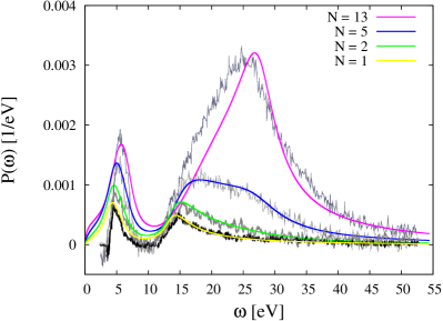
Figure 1: (Color online.) Probability density $P_{N}(\omega)$ (in 1/eV) versus energy loss $\omega$ (in eV), evaluated from Eq. (10) for $N$ = 1, 2, 5, and 13 graphene layers [smooth solid (yellow, green, blue, and pink) curves], along with the corresponding experimental EEL spectra from Ref. Eberlein_2008 [noisy (gray) curves].

Taking $m_{\nu}^{*}$ to be the free electron mass and using the unperturbed surface electron densities of SLG, $n_{\pi}^{0}\approx$ 38 nm^-2 and $n_{\sigma}^{0}=3n_{\pi}^{0}\approx$ 115 nm^-2, we treat the remaining parameters in Eq. (16) as adjustable. The best fit to the experimental EEL spectra Eberlein_2008 is found for $\omega_{\pi r}=4.08$ eV, $\omega_{\sigma r}=13.06$ eV, $\gamma_{\pi}=2.45$ eV, and $\gamma_{\sigma}=2.72$ eV. The results for $P_{N}(\omega)$ were thus computed from Eq. (10) with $N$ = 1, 2, 5 and 13, and are compared in Fig.1 with the experimental curves from Fig. 1(e) of Ref. Eberlein_2008 , corresponding to 1, 2, 5, and $>\!\!10$ graphene layers (We found that our curve $N=13$ provides the best fit with their curve labeled “$>\!$10L”.). We note that the experimental curves were taken under the same acquisition conditions, thereby enabling a direct quantitative comparison among them. Eberlein_2008 On the other hand, apart from adjusting the arbitrary unit of the experimental curves to the absolute unit of our $P_{N}(\omega)$, no relative scaling took place among the theoretical curves with different numbers of layers. One notes that the experimental curves are well reproduced by the LEG model for energies $\omega\gtrsim$ 3 eV and $N<10$, both in magnitude and in the shape of spectra. Regarding the discrepancy at $\omega\lesssim$ 3 eV, we note that the present version of the two-fluid model in Eq. (16), along with the neglect of interlayer tunneling, is only expected to work in MLG for high-energy excitations, but also that the complete vanishing of the experimental spectra at energies below 3 - 4 eV may be a consequence of the method used in their subtraction of the zero-loss peak. Eberlein_2008

Furthermore, while the above values of the parameters $\omega_{\pi r}$, $\omega_{\sigma r}$, $\gamma_{\pi}$, and $\gamma_{\sigma}$ are quite close to those listed in the Table 2 of Ref. Lucas_1995 for the in-plane dielectric function of a 3D, two-fluid model of ADS, features seen in the spectra in Fig.1 are relatively robustly reproduced by theoretical curves for other choices of these parameters. In particular, the damping rates are strongly affected by the presence of impurities or defects, which serve as scattering centers for charge carriers in individual carbon layers. While for graphene on a substrate the concentration of impurities strongly varies from sample to sample, the freestanding graphene may be relatively clean in the case of one or few layers, but thicker samples may contain increased amounts of impurities and defects. Thus, assigning smaller values, or possibly allowing for frequency- dependent damping rates $\gamma_{\pi}$ and $\gamma_{\sigma}$ as in Ref. Djurisic_1999 , could improve the agreement for energies around 10 eV in Fig. 1, where the experiment exhibits an almost complete depletion of the spectra. On the other hand, the width of the high-energy peak at about 27 eV for $N>10$ is not well reproduced by the present choice of parameters, but agreement may be improved if one allows for higher damping rates due to increased density of impurities. Eberlein_2008 This point will be taken up later in the discussion of Fig. 6.

The most important trends seen in Fig. 1 are that the $\pi$ plasmon peak position moves from about 5 eV to about 7 eV as $N$ increases without significant changes in its shape, whereas the $\sigma+\pi$ plasmon peak at about 15 eV for $N=1$ evolves through the development of a plateau between 15 and 27 eV for $N=5$, to be dominated by a peak at about 27 eV for $N=13$, with a growth in magnitude that exceeds the growth of the $\pi$ plasmon peak. The lowest peak positions that occur for $N=1$ and the highest peak positions that occur for $N>10$ in Fig. 1 were associated in Ref. Eberlein_2008 with the surface and bulk plasmon frequencies of graphite, respectively, for both the $\pi$ and $\sigma+\pi$ plasmons. Similarly, we shall see in Fig. 6 that the $\sigma+\pi$ plasmon contributions at about 15 and 27 eV in the EEL spectra of HOPG were also associated in Ref. Carbone_2009a with the surface and bulk plasmons, respectively. In the following, we shall use the LEG model to discuss how adequate those associations are.

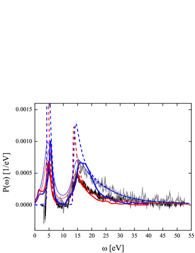
Figure 2: (Color online.) Probability density $P_{N}(\omega)$ (in 1/eV) versus energy loss $\omega$ (in eV), evaluated from Eq. (10) for $N$ = 1 [lower (red) curves] and 2 [upper (blue) curves] graphene layers with non-zero damping (smooth thin solid lines) and vanishing damping (dashed lines), along with the corresponding experimental data [noisy (grey) curves] and the ab initio curves (smooth thick solid lines) from Ref. Eberlein_2008 .

In Fig. 2 we analyze the details of the experimental EEL spectra of Eberlein et al. for $N=1$ and 2, corresponding to a SLG and a bilayer graphene (BLG), which are reproduced from Fig. 1 (noisy curves) along with the theoretical curves from the LEG model for $P_{1}(\omega)$ and $P_{2}(\omega)$ from Eq. (10) (thin solid lines) and with two theoretical curves, taken from Fig. 3(b) of Ref. Eberlein_2008 (thick sold lines), which are based on their ab initio calculations. The most prominent feature of the experimental curves is the asymmetry in the $\sigma+\pi$ plasmon peaks, which is well reproduced by the LEG model, but not by the ab initio calculations by Eberlein et al.Eberlein_2008 (We note, however, that such asymmetry was observed in the ab initio calculations based on a GW and Bethe-Salpeter equation approach by Trevisanutto et al. Trevisanutto_2010 ) We emphasize that the long tails in those peaks, which extend at energies beyond 15 eV, are a consequence of the integration over $q$ in Eq. (10) that captures the effect of dispersion of the $\sigma+\pi$ plasmon, which is neglected when optical limit of the loss function is used. To further elucidate this point, we have recalculated the curves for $P_{1}(\omega)$ and $P_{2}(\omega)$ from Eq. (10) using the same parameters of the two-fluid model in Eq. (16), except that the damping rates of both $\sigma$ and $\pi$ electrons were made very small. The resulting curves are displayed in Fig. 2 by the dashed lines, showing a steep raise at the restoring frequencies $\omega_{\nu r}$, along with the tails that extend for $\omega>\omega_{\nu r}$, giving a very good approximation to the experimental curves at those frequencies.

This observation may be easily rationalized for $N=1$ by referring to the two-fluid model for $\chi_{0}(q,\omega)$ in Eq. (16) in the limit $\gamma_{\sigma}=\gamma_{\pi}\rightarrow 0$, which was discussed in the Appendix C to Ref. Mowbray_2010 . When used in Eq. (10) for $P_{1}(\omega)$, this limit converts the factor $\Im\left[V(q)\chi(q,\omega)\right]$ into a superposition of two $\delta$ functions, $\delta(\omega^{2}-\omega_{\pm}^{2}(q))$, where $\omega_{\pm}(q)$ are the eigenfrequencies describing hybridization between the $\sigma$ and $\pi$ electron fluids in a SLG, which are obtained by solving the equation $\epsilon(q,\omega)=0$ as

$$\begin{array}[]{l}\omega^{2}_{\pm}=\frac{\omega_{\sigma}^{2}+\Omega_{\sigma}^{2}+\omega_{\pi}^{2}+\Omega_{\pi}^{2}}{2}\pm\sqrt{\left(\frac{\omega_{\sigma}^{2}+\Omega_{\sigma}^{2}-\omega_{\pi}^{2}-\Omega_{\pi}^{2}}{2}\right)^{2}+\Omega_{\sigma}^{2}\Omega_{\pi}^{2}},\end{array}$$ (17)

where we define

$$\omega_{\nu}(q)\equiv\sqrt{\omega_{\nu r}^{2}+s_{\nu}^{2}q^{2}}$$ (18)

and

$$\Omega_{\nu}(q)\equiv\sqrt{2\pi e^{2}n_{\nu}^{0}q/m_{\nu}^{*}}$$ (19)

for the $\nu$th fluid. Mowbray_2010 The eigenfrequencies $\omega_{+}(q)$ and $\omega_{-}(q)$ are labeled as the $\sigma+\pi$ and the $\pi$ plasmon modes of SLG, and the corresponding dispersion relations are shown in Fig. 3 by the upper and lower dotted lines, respectively. For the purpose of the present discussion, it suffices to expand the expressions in Eq. (17) to the first order in $q$, so that $\omega_{+}^{2}\approx\omega_{\sigma r}^{2}+\Omega_{\sigma}^{2}(q)$ and $\omega_{-}^{2}\approx\omega_{\pi r}^{2}+\Omega_{\pi}^{2}(q)$, describing the long wavelength behavior of plasmon frequencies of the non-interacting $\sigma$ and $\pi$ fluids in SLG. Using these expressions for $\omega_{\pm}^{2}(q)$ in the delta functions $\delta(\omega^{2}-\omega_{\pm}^{2}(q))$ makes the integration over $q$ in Eq. (10) trivial, giving two contributions to $P_{1}(\omega)$ of the form $\sim n_{\nu}^{0}/(\omega^{2}-\omega_{\nu r}^{2})$, which essentially capture the behavior of the tails seen in Fig. 2 for $\omega^{2}-\omega_{\nu r}^{2}\gg 2\pi e^{2}n_{\nu}^{0}\omega/\left(m_{\nu}^{*}v_{\perp}\right)$.

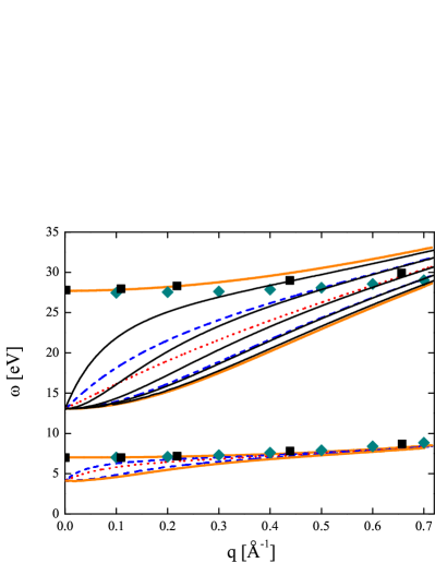
Figure 3: (Color online.) Dispersion curves for the $\pi$ (lower group) and $\sigma+\pi$ (upper group) plasmons in MLG, obtained from the LEG model with $N=1$ [dotted (red) lines] and $N=2$ [dashed (blue) lines], as well as $N=5$ [only the upper group is shown by (black) solid lines]. The upper and the lower edges are shown for both the $\pi$ and $\sigma+\pi$ plasmon bands in HOPG [thick (orange) solid lines]. The (dark cyan) diamonds show the experimental plasmon peak positions in the EEL spectra of HOPG from Ref. Kramberger_2010 , whereas the (black) squares show the peak positions obtained by ab initio calculations for graphite in Ref. Marinopoulos_2004 .

Furthermore, it is interesting to comment on the similarity between the experimental spectra for BLG and SLG, seen in Fig. 2. In particular, their high-frequency tails at $\omega\gtrsim 20$ eV seem to imply a scaling ratio of about 2:1, as remarked by Eberlein et al.. Eberlein_2008 This is best rationalized by resorting to the eigenmode analysis for BLG by setting $\gamma_{\sigma}=\gamma_{\pi}\rightarrow 0$ in Eq. (10) for $P_{2}(\omega)$. Then, it can be shown that the factor $\Im\left[V(q)\chi(q,\omega)Q_{2}(q,\omega)\right]$ becomes singular at four frequencies, which are given by the expressions in Eq. (17) when frequencies $\Omega_{\nu}(q)$ in Eq. (19) are replaced by $\Omega_{\nu}^{\pm}(q)\equiv\Omega_{\nu}(q)\sqrt{1\pm\exp(-qd)}$. The corresponding dispersion curves are shown in Fig. 3 by the dashed lines, two in the upper ($\sigma+\pi$ plasmon) group and two in the lower ($\pi$ plasmon) group. However, the weakly (quadratically) dispersing lower curves in each plasmon group contribute to $P_{2}(\omega)$ with negligible spectral weights because of the smallness of the factor $\omega d/v_{\perp}$ at the frequencies of interest here. Namely, by setting $\cos\left(\omega d/v_{\perp}\right)\approx 1$ in Eq. (12), one obtains $Q_{2}(q,\omega)\approx 2/\left[1+V(q)\chi(q,\omega)\exp(-qd)\right]$, so that the dominant spectral weight in $P_{2}(\omega)$ comes mostly from the upper (linearly dispersing) curves in the $\sigma+\pi$ and $\pi$ plasmon groups, seen in Fig. 3 for BLG. This may be further simplified by noting that the kinematic factor $K^{2}(q,\omega)$ is strongly peaked at $q=\omega/v_{\perp}$, so that $\exp(-qd)\approx 1$, and hence the factor $\Im\left[V(q)\chi(q,\omega)Q_{2}(q,\omega)\right]$ in Eq. (10) for $P_{2}(\omega)$ becomes $-\Im\left\{1/\left[1+2V(q)\chi_{0}(q,\omega)\right]\right\}$, corresponding to a SLG with doubled $\sigma$ and $\pi$ electron densities. Accordingly, the slopes of the upper dispersion curves for BLG in the $\sigma+\pi$ and $\pi$ plasmon groups are seen in Fig. 3 to be about twice the slopes of the corresponding dispersion curves for SLG in the limit of long wavelengths. As a consequence, the peak positions in $P_{2}(\omega)$ occur at about the same frequencies as those in $P_{1}(\omega)$, whereas the high-frequency tails in $P_{2}(\omega)$ are approximated by $\sim 2n_{\nu}^{0}/(\omega^{2}-\omega_{\nu r}^{2})$, confirming their ratio of 2:1 relative to the tails in $P_{1}(\omega)$.

The above analysis of SLG and BLG shows that various eigenmodes of the underlying structure enter the EEL spectra with weights that are strongly dependent on the incident electron speed. This dynamic aspect of the LEG model, which is not covered in the ab initio calculations, Eberlein_2008 is related to the interference effect in plasmon excitations at different carbon layers within a MLG, and it may be quantified by the factor $\omega T_{N}$ that appears in the expression for $Q_{N}(q,\omega)$, cf. Eqs. (5), (7) and (11), where $T_{N}\equiv Nd/v_{\perp}$ is the time it takes the incident electron to traverse the full thickness of MLG (neglecting relativistic effects). Therefore, the interference effect will be negligible for fast incident electrons in STEM at frequencies of interest in the low-loss EELS of MLGs with a few layers giving $\omega T_{N}\ll 1$. The smallness of the factor $\omega T_{N}=Nd\omega/v_{\perp}$ is equivalent to the limit $d\rightarrow 0$, giving a picture where all layers collapse onto a single sheet or, equivalently, the in-plane plasmon modes in all layers oscillate in phase, which explains the similarity among the spectra and the approximate scaling of their high-energy tails as $P_{N}\propto N$ for $N\sim 1$. In other words, the EEL spectra of MLGs with $N=2,3,\ldots$ are dominated by the peaks that are derived from the $\pi$ and $\sigma+\pi$ plasmons of SLG, and hence they should not be associated with the surface plasmons of graphite. Eberlein_2008

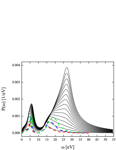
Figure 4: (Color online.) Probability density $P_{N}(\omega)$ (in 1/eV) versus energy loss $\omega$ (in eV), evaluated from Eq. (10) for $N$ in the range from 1 to 15 with unit steps, using the same parameters as in Fig. 1 [solid (black) curves]. Also shown are the results of ab initio calculations from Ref. Eberlein_2008 for graphene with $N=1,2$, and 3 layers [dashed (red, blue, and green, respectively) curves].

When $N\gtrsim 10$, the factor $\omega T_{N}=Nd\omega/v_{\perp}$ may no longer be small, and hence the interference effect may become significant in sufficiently thick MLGs. Obviously, the onset of the interference effect will occur at a smaller $N$ if the incident electron moves at a lower speed. Moreover, because of the difference in the relevant frequency ranges, one expects that the interference effect will be more prominent for the $\sigma+\pi$ than for the $\pi$ plasmons. This may explain why the $\sigma+\pi$ plasmon peak in Fig. 1 undergoes a more substantial change with increasing $N$ than the $\pi$ plasmon peak. To illustrate this point, we show in Fig. 4 a detailed evolution of the EEL spectra $P_{N}(\omega)$ from Eq. (10) for $N$ going from 1 to 15 in unit steps, which were calculated with the same parameters of the two-fluid model in Eq. (16) as those used in Fig. 1. (For the sake of further comparison with ab initio calculations, we also show in our Fig. 4 the results from Fig. 3(b) of Ref. Eberlein_2008 for the in-plane spectra of graphene with $N=1,2$, and 3 layers.) One confirms in Fig. 4 that in the LEG model the $\pi$ plasmon peak moves continuously from about 5 to about 7 eV as $N$ increases, whereas the spectral structure associated with the $\sigma+\pi$ plasmon appears to evolve as a superposition of two peaks, one at about 15 eV and the other at about 27 eV, which do not move much as $N$ increases but rather have their weights strongly dependent on $N$. One may further see from Fig. 4 that the contribution from the peak at about 15 eV dominates the spectra for $N\lesssim 5$, and is still visible for $N\lesssim 10$, whereas the spectra with $N>10$ are dominated by the peak at about 27 eV. In particular, it appears in Fig. 4 that the weights of those two peaks are approximately equal for MLG with $N=6$ layers, giving a value of the relevant interference factor of $\omega T_{6}\approx 0.5$. Such a peculiar composition of the $\sigma+\pi$ plasmon peak for $N\sim$ 5 - 6 deserves further analysis.

One expects that the plasmon eigenfrequencies in MLG with finite $N$ will fall into two disjoint groups, each giving $N$ dispersion curves that correspond to the $\sigma+\pi$ and $\pi$ plasmons of SLG. All the curves within each group become degenerate as $q\rightarrow 0$ and they approach the corresponding restoring frequencies of SLG, $\omega_{\sigma r}$ and $\omega_{\pi r}$, but they spread out at finite $q$, forming two quasibands. Giuliani_1983 ; Jain_1985 In Fig. 3 we show such a quasi-band for $N=5$ in the $\sigma+\pi$ group (the corresponding quasi-band in the $\pi$ group is not shown to avoid cluttering of curves in that group). Similar quasibands may be seen in the case of MWCNTs with, e.g., $N=30$ walls in Fig. 4(a) of Ref. Yannouleas_1996 based on a single-fluid model for $\sigma$ electrons, and $N=10$ walls in Fig. 1 of Ref. Chung_2007 based on a two-fluid model for both $\sigma$ and $\pi$ electrons. One sees in Fig. 3 that the four lower curves in the $\sigma+\pi$ quasi-band for $N=5$ are quadratically dispersing, whereas the uppermost curve is linearly dispersing with a slope that is about five times the slope of the corresponding $N=1$ curve for small $q$. It can be shown that, by setting $\cos\left(\omega d/v_{\perp}\right)\approx 1$ as in the case with $N=2$, the uppermost curve in the $\sigma+\pi$ quasi-band for $N=5$ gives the dominant contribution to the spectrum $P_{5}(\omega)$. The large initial slope of that dispersion curve, along with its tendency to saturate for higher $q$ values, gives rise to a high-energy tail in $P_{5}(\omega)$ that forms a bump at about 27 eV, which is clearly seen in the experimental spectrum for $N=5$ in Fig. 1. As $N$ further increases, this saturation of the dispersion curves within a quasi-band becomes more prominent because of a well-defined upper bound, Yannouleas_1996 which is best illustrated by resorting to the eigenmode analysis of an infinite periodic lattice of SLGs.

In the limit $N\rightarrow\infty$ we recover the case of HOPG, which exhibits two bands of dispersion relations corresponding to the $\sigma+\pi$ and $\pi$ bulk plasmon modes. They are obtained by letting $0\leq k\leq\pi/d$ and solving the equation in Eq. (15) with $\chi_{0}(q,\omega)$ from the two-fluid model of Eq. (16) where $\gamma_{\sigma}=\gamma_{\pi}\rightarrow 0$. Giuliani_1983 ; Jain_1985 ; Shung_1986 ; Gumbs_1988 The upper and the lower edges of those bands are defined by $k=0$ and $k=\pi/d$, respectively, and the corresponding dispersion relations are given by $\omega=\omega_{\pm}^{\mathrm{up}}(q)$ and $\omega=\omega_{\pm}^{\mathrm{low}}(q)$ with “+” for the $\sigma+\pi$ plasmon band and “-” for the $\pi$ plasmon band, where expressions in Eq. (17) are to be used with the frequencies $\Omega_{\nu}(q)$ in Eq. (19) replaced by $\Omega_{\nu}^{\mathrm{up}}(q)=\Omega_{\nu}(q)\sqrt{\coth(qd/2)}$ and $\Omega_{\nu}^{\mathrm{low}}(q)=\Omega_{\nu}(q)\sqrt{\tanh(qd/2)}$. Those band edges are shown by the four thick solid (orange) curves in Fig. 3, which all exhibit parabolic dispersions in the long wavelength limit.

When $q\rightarrow 0$, one can show that the lower band edges in Fig. 3 approach the restoring frequencies of SLG, $\omega_{+}^{\mathrm{low}}(0)=\omega_{\sigma r}$ and $\omega_{-}^{\mathrm{low}}(0)=\omega_{\pi r}$, whereas the upper band edges approach the values $\omega_{\pm}^{\mathrm{up}}(0)$ that are given by $\omega_{\pm}$ in Eq. (17) when the frequencies $\Omega_{\nu}(q)$ in Eq. (19) are replaced by $\Omega_{\nu p}=\sqrt{4\pi e^{2}N_{\nu}^{0}/m_{\nu}^{*}}$, corresponding to the bulk plasmon frequency in the $\nu$th electron fluid with an effective volume density of $N_{\nu}^{0}\equiv n_{\nu}^{0}/d$. Using our parameters from Fig. 1, we find $\Omega_{\sigma p}\approx$ 21.7 eV and $\Omega_{\pi p}\approx$ 12.5 eV, which are quite close to the plasmon frequencies listed in the Table 2 of Ref. Lucas_1995 for the in-plane dielectric function of the ADS model. Hence, we obtain for the long wavelength limits of the upper edges of the bulk $\sigma+\pi$ and $\pi$ plasmon bands in Fig. 3 the values $\omega_{+}^{\mathrm{up}}(0)\approx 27.7$ eV and $\omega_{-}^{\mathrm{up}}(0)\approx 7$ eV, respectively, which are remarkably close to the peak positions seen in the $P_{N}(\omega)$ curves in Figs. 1 and 4 for $N>10$. This may be rationalized by referring to the $N\rightarrow\infty$ limit of the LEG model, given in Eq. (13), where we see that the smallness of the factor $kd=\omega d/v_{\perp}$ in $S(q,k)$, cf. Eq. (14) implies that the dominant spectral weights in $P_{\infty}(\omega)$ come from the upper edges (defined by $k=0$) of the bulk $\sigma+\pi$ and $\pi$ plasmon bands of HOPG.

Hence, for finite $q$, one expects that the peak positions of both the $\pi$ and $\sigma+\pi$ plasmons in the EEL spectra of HOPG should closely follow the dispersion relations of the upper edges of the corresponding plasmon bands. This is corroborated in Fig. 3 by a comparison with the peak positions taken from Figs. 3 and 5 of Ref. Kramberger_2010 , which were deduced from the experimental EEL spectra of HOPG. (We note that the overdispersion of the $\sigma+\pi$ upper band edge relative to the experimental points at larger $q$ values in Fig. 3 may be reduced if a finite damping rate is introduced in the two-fluid model.) In addition, we display in Fig. 3 the peak positions obtained in Ref. Marinopoulos_2004 from ab initio calculations for graphite, showing good agreement with both the experimental data Kramberger_2010 and the upper edges of the plasmon bands. Therefore, the previously mentioned association of the plasmon peaks in the EEL spectra of thick samples of MLG or HOPG with the bulk plasmon modes of graphite Eberlein_2008 ; Carbone_2009a should be made more specific by stressing that it is the upper edges of the bulk plasmon bands that give the prevalent contributions to the EEL spectra of such structures.

On the other hand, for incident electrons at lower speeds, one expects that increased contributions in the plasmon spectra of HOPG may also come from the portions of the bulk plasmon bands with lower energies. In that context, we mention that Fig. 1 in Ref. Baitinger_2006 shows the results of a HREELS experiment on HOPG using a 200 eV incident electron beam, where contributions from the entire $\sigma+\pi$ plasmon band are seen to strongly depend on the electron reflection angle. In particular, a prominent peak was observed in the spectra at about 13 - 14 eV that did not move much when the reflection angle was changed. Baitinger_2006 While that peak was associated by the author with a surface plasmon, its presence may be alternatively explained as resulting from a van-Hove type of singularity in the plasmon density of states at the lower band edge of the $\sigma+\pi$ plasmon band. Morawitz_1993 Clearly, further investigation into the features of high-energy spectra of HOPG in HREELS is warranted.

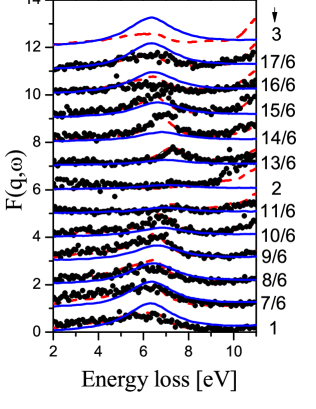
Figure 5: (Color online.) Dynamic structure factor [solid (blue) lines] is evaluated from Eq. (20) and appropriately scaled to compare it with the corresponding experimental IXS data (points) from Ref. Hambach_2008 with a fixed in-plane wavenumber of $q=$ 0.37 Å^-1 for the indicated values of the perpendicular wavenumber $k$. Also shown are the results of ab initio calculations from Ref. Hambach_2008 [dashed (red) lines].

It is worthwhile mentioning that the $\pi$ plasmon band was probed in a recent experiment by Hambach et al., Hambach_2008 who used IXS to measure the frequency dependent dynamic structure factor (DSF) of HOPG for momentum transfers beyond its first Brillouin zone. The experimental data from Fig. 3(a) in Ref. Hambach_2008 are reproduced in our Fig. 5, along with the results from their ab initio calculations, showing the frequency dependence of a region near the $\pi$ plasmon peak for a range of perpendicular wave numbers, $\pi\leq kd\leq 3\pi$, with a fixed in-plane wave vector component of about 0.37 Å^-1. In particular, the peak position is seen to oscillate between the values of about 6 and 7 eV, which are commensurate with the extent of the $\pi$ plasmon band in our Fig. 3 when one sets $q=$ 0.37 Å^-1 and invokes graphene’s nearly isotropic in-plane polarizability. Furthermore, one can show that the DSF of an infinite periodic lattice is proportional to the factor

$$F(q,\omega)=\Im\!\left[\frac{V(q)\chi_{0}(q,\omega)}{1+S\!\left(q,k\right)V(q)\chi_{0}(q,\omega)}\right],$$ (20)

which appears in Eq. (13) with $S(q,k)$ defined in Eq. (14). By using the same parameters as those used in Fig. 1, one can easily evaluate from Eq. (20) a set of spectral curves for HOPG with $q=$ 0.37 Å^-1 for a range of $kd$ values, which are seen in Fig. 5 to reproduce all the main features of the corresponding experimental data and ab initio results for DSF from Ref. Hambach_2008 , including the $\pi$ plasmon peak position variation with $kd$, and its near disappearance for $kd=2\pi$. We take that this comparison demonstrates both the validity of the concept of plasmon bands in HOPG and the ability of the LEG model to describe them in a simple analytical manner.

Regarding the applicability of the $N\rightarrow\infty$ limit of the LEG model in the context of EELS in STEM, we obviously require $\omega T_{N}\gg 1$ because, in view of the strong peaking of the kinematic factor at $q=\omega/v_{\perp}$ in $P_{\infty}(\omega)$ from Eq. (13), this condition amounts to $Ndq\gg 1$, which guarantees that the end effects are negligible. When $\omega T_{N}\sim 1$, the interference is strong and the end effects in such MLG may not be neglected, making it necessary to use $P_{N}(\omega)$ from Eq. (10), even when $N\gg 1$. To illustrate this point, we mention that, when attempting to model in Fig. 1 the experimental EEL spectra for the thickest MLG from Ref. Eberlein_2008 with “$>\!\!10$” layers, we could not obtain nearly as good a fit with $P_{\infty}(\omega)$ as we did with $P_{N}(\omega)$ for $N=13$. The fact that the interference factor in this case takes the value $\omega T_{13}\approx 1$ points to a need to look elsewhere for the experimental EEL spectra of thick enough MLG, where we may test the applicability of $P_{\infty}(\omega)$ from Eq. (13) to HOPG.

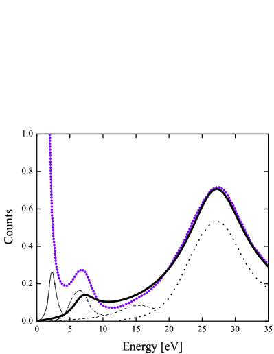
Figure 6: (Color online.) The EEL spectra versus energy loss (in eV), evaluated from $P_{\infty}(\omega)$ in Eq. (13) [thick (black) solid line], along with the corresponding experimental spectrum of HOPG from Ref. Carbone_2009a [the (violet) chain curve], which is theoretically decomposed into a laser-generated peak [thin (black) solid line], $\pi$ plasmon peak [thin (black) dash-dot line], a “surface” $\sigma+\pi$ plasmon peak [thin (black) dashed line], and a “bulk” $\sigma+\pi$ plasmon peak [thin (black) dotted line].

In that context, we find it instructive to model the recent experiment by Carbone et al., Carbone_2009a who used their UEM in the so-called static mode to obtain the EEL spectra of a slab of HOPG, having such a thickness that $\omega T_{N}\approx 20$. In Fig. 6 we compare the experimental curve from Fig. 2 of Ref. Carbone_2009a for HOPG with our result for the (appropriately scaled) probability density $P_{\infty}(\omega)$ from Eq. (13), where we used the two-fluid model for $\chi_{0}(q,\omega)$ given in Eq. (16). In order to achieve the best fit with the experiment, we used the same parameters for the $P_{\infty}(\omega)$ curve in Fig. 6 as those used for the $P_{N}(\omega)$ curves in Figs. 1 and 4, except for $\gamma_{\sigma}$, which was increased to $\gamma_{\sigma}=9.52$ eV to take into account that the damping rate for $\sigma$ electrons may be increased due to more abundant impurities or defects in a thick slab of HOPG than in a few-layer MLG. Our curve for $P_{\infty}(\omega)$ is seen in Fig. 6 to reproduce the experiment very well for energies $\gtrsim 10$ eV due to the increased parameter $\gamma_{\sigma}$, whereas the $\pi$ plasmon peak is only qualitatively reproduced in shape, but its position fits the experiment well. The discrepancy between our model and the experiment at energies $\lesssim 10$ eV may be partially ascribed to the presence of both the zero-loss peak and the photogenerated charge carrier plasma excitations at around 2.4 eV, which were not subtracted from the experimental curve in Ref. Carbone_2009a . We also show in Fig. 4 a phenomenological decomposition of the experimental curve into four theoretical curves, which was performed in Ref. Carbone_2009a . Those curves describe contributions from several processes that were associated by the authors with: the laser-generated region peaked at about 2.4 eV, the $\pi$ plasmon peaked at about 7 eV, the surface $\sigma+\pi$ plasmon peaked at about 15 eV with a low weight, and the bulk $\sigma+\pi$ plasmon peaked at about 27 eV with a much larger weight than its surface counterpart. Carbone_2009a While such a decomposition of the $\sigma+\pi$ plasmon contributions is corroborated by the above analysis, we believe that it would be more adequate to label the peaks at 15 and 27 eV as contributions related to the lower edge (which carries a signature of the SLG’s $\sigma+\pi$ plasmon mode) and the upper edge of the bulk $\sigma+\pi$ plasmon band in HOPG, respectively.

IV Concluding remarks

We have shown that a simple and straightforward implementation of the LEG model Fetter_1974 ; Giuliani_1983 ; Jain_1985 to MLG gives analytical expressions for the spectra of the energy lost by a fast electron under normal incidence that provide an explicit account of the effect of increasing number $N$ of graphene layers on the high-energy plasmon excitations in MLG. Those expressions are given in terms of a single-layer polarizability $\chi_{0}(q,\omega)$ that may be modeled independently from the LEG model. By adopting a phenomenological, two-dimensional, two-fluid model for $\chi_{0}(q,\omega)$, which includes Lorentz parameters suitable for describing the dominant $\pi\rightarrow\pi^{*}$ and $\sigma\rightarrow\sigma^{*}$ inter-band transitions in SLG, we found good agreement with the plasmon spectra from four independent experiments. In particular, the shape of such spectra was well reproduced for MLG with $N\lesssim$ 10, where the most dramatic change occurs in the $\pi$ and $\sigma+\pi$ plasmon peaks. Eberlein_2008 In addition, it was shown that the experimental EEL spectra for both MLG with $N>10$ Eberlein_2008 and a thick slab of HOPG Carbone_2009a may be well reproduced by the same model by allowing for increased damping rates in $\chi_{0}(q,\omega)$.

Specifically, the LEG model reproduced the experimentally determined peak positions, Eberlein_2008 which were found to move from about 5 to about 7 eV for the $\pi$ plasmon and from about 15 to about 27 eV for the $\sigma+\pi$ plasmon as the number of layers in MLG grows from $N\sim 1$ to $N>10$. Eberlein_2008 By referring to the eigenmode analysis of the underlying MLG structures, both the plasmon peak positions and the experimentally observed similarity among the EEL spectra for $N=1,2,3,\ldots$ were found to be derived from the plasmon spectra of SLG, based on the smallness of the factor $\omega d/v_{\perp}$ under typical experimental conditions (low loss EELS and the 100 keV incident electrons with $d\approx$ 3.35 Å^-1). Eberlein_2008 Hence no association with the surface plasmons of graphite seems to be justified for the peaks at about 5 and about 15 eV for the $\pi$ and $\sigma+\pi$ plasmons, respectively, in MLG with few layers. In addition, the high-frequency tails in the experimental EEL spectra were exactly reproduced by the LEG model for $N=1$ and 2, and were identified as arising from the plasmon dispersion and from integration over a large range of the in-plane wave numbers, commensurate with the experimental conditions. Eberlein_2008

On the other hand, for sufficiently thick MLG, such that $Nd\omega/v_{\perp}\gg 1$, the limit of an infinite periodic lattice of SLGs showed that the peaks at about 7 and about 27 eV come predominantly from the upper edges of the $\pi$ and $\sigma+\pi$ plasmon bands in the bulk of HOPG, respectively, again because of the smallness of the factor $\omega d/v_{\perp}$. This seems to be corroborated by a comparison with the experimental dispersion relations found from the EEL spectra of graphite. Kramberger_2010 Moreover, it was shown that the $N\rightarrow\infty$ limit of the LEG model also gives good account of a dynamic structure factor that was measured by IXS of HOPG, Hambach_2008 reproducing the movement of the $\pi$ plasmon peak between the corresponding $\pi$ plasmon band edges.

When $Nd\omega/v_{\perp}\sim 1$, the $\sigma+\pi$ plasmon peak is seen to evolve through a sequence of broad structures between 15 and 27 eV, Eberlein_2008 which result from the development of a quasiband of plasmon dispersion curves for MLG with $N\sim 10$ that is a precursor to a fully developed bulk $\sigma+\pi$ plasmon band of HOPG. Furthermore, having in mind that the underlying semi-infinite lattice of SLGs for $N\rightarrow\infty$ does not support surface states in HOPG placed in the air or vacuum, Giuliani_1983 ; Jain_1985 one may conclude that any remaining trace of the peak at about 15 eV for the $\sigma+\pi$ plasmon in the EEL spectra of HOPG is likely to be related to the lower edge of its bulk $\sigma+\pi$ plasmon band, Carbone_2009a and not to a surface plasmon of graphite.

Given that small variations in the free parameters, used in the model adopted for $\chi_{0}(q,\omega)$, do not corrupt the agreement found with the four independent experiments, Eberlein_2008 ; Carbone_2009a ; Hambach_2008 ; Kramberger_2010 we suggest that using the LEG model for high-energy plasmon excitations in MLG, HOPG, and other multilayer carbon nanostructures indeed presents a versatile and robust alternative to other theoretical approaches. The novel applications of these analytical models, presented in this work shed light on several aspects of the problem at hand, including (a) the role of plasmon dispersion in the spectra integrated over the wave number, (b) the role of the dynamical interference factor $Nd\omega/v_{\perp}$ in determining which eigenmodes of the underlying MLG structure have prevalent spectral weights, and (c) the relevance of the bulk plasmon bands, rather than surface plasmons, in classifying the observed plasmon peak frequencies.

- (1) M. H. Gass, U. Bangert, A. L. Bleloch, P. Wang, R. R. Nair, and A. K. Geim, Nat. Nanotechnol. 3, 676 (2008).
- (2) T. Eberlein, U. Bangert, R. R. Nair, R. Jones, M. Gass, A. L. Bleloch, K. S. Novoselov, A. Geim, and P. R. Briddon, Phys. Rev. B 77, 233406 (2008).
- (3) F. Carbone, B. Barwick, O. H. Kwon, H. S. Park, J. S. Baskin, and A. H. Zewail, Chem. Phys. Lett. 468, 107 (2009).
- (4) F. Carbone, O. H. Kwon, and A. H. Zewail, Science 325, 5937 (2009).
- (5) R. Hambach, C. Giorgetti, N. Hiraoka, Y. Q. Cai, F. Sottile, A. G. Marinopoulos, F. Bechstedt, and L. Reining, Phys. Rev. Lett. 101, 266406 (2008).
- (6) J. P. Reed, B. Uchoa, Y. I. Joe, Y. Gan, D. Casa, E. Fradkin, and P. Abbamonte, Science 330, 805 (2010).
- (7) M. H. Upton, R. F. Klie, J. P. Hill, T. Gog, D. Casa, W. Ku, Y. Zhu, M. Y. Sfeir, J. Misewich, G. Eres, and D. Lowndes, Carbon 47, 162 (2009).
- (8) P. B. Visscher and L. M. Falicov, Phys. Rev. B 3, 2541 (1971).
- (9) A. L. Fetter, Annals of Physics 88, 1 (1974).
- (10) G. F. Giuliani and J. J. Quinn, Phys. Rev. Lett. 51, 919 (1983).
- (11) J. K. Jain and P. B. Allen, Phys. Rev. Lett. 54, 2437 (1985).
- (12) G. Gumbs, Phys. Rev. B 37, 10184 (1988).
- (13) K. W.-K. Shung, Phys. Rev. B 34, 979 (1986).
- (14) V. Z. Kresin and H. Morawitz, Phys. Rev. B 37, 7854 (1988).
- (15) H. Morawitz, I. Bozovic, V. Z. Kresin, G. Rietveld, and D. van der Marel, Z. Phys. B 90, 277 (1993).
- (16) C. Yannouleas, E. N. Bogachek, and U. Landman, Phys. Rev. B 53, 10225 (1996).
- (17) S. Chung, D. J. Mowbray, Z. L. Miskovic, F. O. Goodman, and Y.-N. Wang, Radiat. Phys. Chem. 76, 524 (2007).
- (18) A. G. Marinopoulos, L. Reining, A. Rubio, and V. Olevano, Phys. Rev. B 69, 245419 (2004).
- (19) A. A. Lucas, L. Henrard, and Ph. Lambin, Nucl. Instrum. Methods Phys. Res. B 96, 470 (1995).
- (20) M. Kociak, L. Henrard, O. Stephan, K. Suenaga, and C. Colliex, Phys. Rev. B 61, 13936 (2000).
- (21) D. Taverna, M. Kociak, V. Charbois, and L. Henrard, Phys. Rev. B 66, 235419 (2002).
- (22) O. Stephan, D. Taverna, M. Kociak, K. Suenaga, L. Henrard, and C. Colliex, Phys. Rev. B 66, 155422 (2002).
- (23) O. H. Crawford, Phys. Rev. A 42, 1390 (1990).
- (24) I. Villo-Perez, Z. L. Miskovic, and N. R. Arista, in Trends in Nanoscience: Theory, Experiment, Technology, edited by. A. Aldea and V. Barsan, (Springer, Berlin, 2010), p. 217.
- (25) A. Nagashima, K. Nuka, H. Itoh, T. Ichinokawa, C. Oshima, S. Otani, and Y. Ishizawa, Solid State Commun. 83, 581 (1992).
- (26) A. H. Castro Neto, F. Guinea, N. M. Peres, K. S. Novoselov, and A. K. Geim, Rev. Mod. Phys. 81, 109 (2009).
- (27) S. Das Sarma, S. Adam, E. H. Hwang, and E. Rossi, Rev. Mod. Phys. 83, 407 (2011).
- (28) E. H. Hwang, R. Sensarma, and S. Das Sarma, Phys. Rev. B 82, 195406 (2010).
- (29) Y. Liu, R. F. Willis, K. V. Emtsev, and Th. Seyller, Phys. Rev. B 78, 201403(R) (2008).
- (30) T. Langer, J. Baringhaus, H. Pfnür, H. W. Schumacher, and C. Tegenkamp, New J. Phys. 12, 033017 (2010).
- (31) Y. Liu and R. F. Willis, Phys. Rev. B 81, 081406(R) (2010).
- (32) T. Langer, D. F. Förster, C. Busse, T. Michely, H. Pfnür, and C. Tegenkamp, New J. Phys. 13, 053006 (2011).
- (33) K. F. Allison, D. Borka, I. Radovic, Lj. Hadzievski, and Z. L. Miskovic, Phys. Rev. B 80, 195405 (2009).
- (34) K. F. Allison and Z. L. Miskovic, Nanotechnology 21, 134017 (2010).
- (35) R. F. Egerton, Rep. Prog. Phys. 72, 016502 (2009).
- (36) P. E. Trevisanutto, M. Holzmann, M. Cote, and V. Olevano, Phys. Rev. B 81, 121405(R) (2010).
- (37) Z. Chen and X.-Q. Wang, Phys. Rev. B 83, 081405(R) (2011).
- (38) L. Yang, Phys. Rev. B 83, 085405 (2011).
- (39) J. Cazaux, Solid State Commun. 8, 545 (1970).
- (40) D. J. Mowbray, S. Segui, J. Gervasoni, Z. L. Miskovic, and N. R. Arista, Phys. Rev. B 82, 035405 (2010).
- (41) L. Calliari, S. Fanchenko, and M. Filippi, Carbon 45, 1410 (2007).
- (42) L. Calliari, S. Fanchenko, and M. Filippi, Surf. Interface Anal. 40, 814 (2008).
- (43) D. Drosdoff and L. M. Woods, Phys. Rev. B 82, 155459 (2010).
- (44) G. Barton and C. Eberlein, J. Chem. Phys. 95, 1512 (1993).
- (45) D. A. Gorokhov, R. A. Suris, and V. V. Cheianov, Phys. Lett. A 223, 116 (1996).
- (46) X. D. Jiang, Phys. Rev. B 54, 13487 (1996).
- (47) D. J. Mowbray, Z. L. Miskovic, F. O. Goodman, and Y.-N. Wang, Phys. Rev. B 70, 195418 (2004).
- (48) C. Kramberger, R. Hambach, C. Giorgetti, M. H. Rümmeli, M. Knupfer, J. Fink, B. Büchner, L. Reining, E. Einarsson, S. Maruyama, F. Sottile, K. Hannewald, V. Olevano, A. G. Marinopoulos, and T. Pichler, Phys. Rev. Lett. 100, 196803 (2008).
- (49) A. B. Djurisic and E. H. Li, J. Appl. Phys. 85, 7404 (1999).
- (50) C. Kramberger, E. Einarsson, S. Huotari, T. Thurakitseree, S. Maruyama, M. Knupfer, and T. Pichler, Phys. Rev. B 81, 205410 (2010).
- (51) E. M. Baitinger, Phys. Solid State 48, 1461 (2006).