Density profile of interacting Fermions in a one-dimensional optical trap

Abstract

The density distribution of the one-dimensional Hubbard model in a harmonic trapping potential is investigated in order to study the effect of the confining trap. Strong superimposed oscillations are always present on top of a uniform density cloud, which show universal scaling behavior as a function of increasing interactions. An analytical formula is proposed on the basis of bosonization, which describes the density oscillations for all interaction strengths. The wavelength of the dominant oscillation changes with interaction, which indicates the crossover to a spin-incoherent regime. Using the Bethe ansatz the shape of the uniform fermion cloud is analyzed in detail, which can be described by a universal scaling form.

Ultra-cold gases in optical traps and lattices have become a promising tool for simulating strongly correlated systems with a full control of all relevant parameters review . While the first simulations were mostly made on bosonic setups, ultra-cold fermions are by now also well established fermions . In order to simulate interacting electron systems such as Hubbard-type models, fermionic atoms with two different hyperfine states are used in order to represent the two spin channels fermions . It is therefore possible to test theoretical predictions even for systems that are less common or hard to produce in nature, such as perfectly clean isolated one-dimensional (1D) quantum wires. However, the experimental setup will always possess a smoothly varying potential due to the intensity profile of the laser beams, usually forming a harmonic confinement.

Recent experimental developments have made it possible to locally probe the density profile of ultra-cold atomic condensates directly in space using optical microscopy kuhr or electron beam scanning ott . In this work we therefore want to provide a detailed theoretical quantitative analysis of the 1D fermion density profile as a function of the interaction strength and the confining potential, which in turn can be used to analyze interaction effects from the experimental signals.

The fermion density can generally be characterized in terms of two distinct features, namely the overall size of the cloud on the one hand and superimposed density oscillations on the other hand. From works on quantum wires and quantum dots it is well known that density oscillations may appear from reflections at sharp edges and boundaries, which are due to interference (Friedel oscillations) and/or localization (Wigner crystallization) friedel ; mueller ; Soffing09 ; Bedurftig98 ; rommer ; White02 . However, it is not a priori clear how these oscillations are modified if a harmonic potential is present as a confinement. In this work we now show that the oscillations remain strong in a harmonic trap with interactions, despite the lack of any sharp edges which may cause Friedel oscillations. In a pioneering work schulz from 1993, Schulz predicted $4k_{F}$ density correlations to dominate, which he called a one-dimensional ”Wigner crystal”, that only occurs in case that the interaction parameter takes on rather extreme values, which cannot be reached in a short-ranged Hubbard model even for infinite $U$. In contrast to this expectation, we now find a surprising crossover towards rather strong $4k_{F}$ ”Wigner oscillations” in a trap even for intermediate short-range interactions. Moreover, both Friedel and Wigner oscillations can actually be very well analyzed with the help of an analytic formula on the basis of a bosonization approach. The overall size and shape of the density cloud is also analyzed in quantitative detail, which follows a universal scaling form.

We consider the standard 1D Hubbard Hamiltonian with an external trapping potential

$$H=\sum_{x}\sum_{\sigma=\uparrow,\downarrow} \!\!\!\!\!\!\!\!\left(-J(\psi_{\sigma,x}^{\dagger}\psi_{\sigma,x+1}^{\phantom{\dagger}}+\text{h.c.})\right.$$ (1)

$$\left.+(\mu_{0}+\omega^{2}x^{2})\,n_{\sigma,x}+\frac{U}{2}n_{\sigma,x}n_{\sigma,x}\right)$$

in the limit of large particle separations (small densities) relative to the lattice spacing. In this limit muth the Hamiltonian can also be approximated by the continuous problem of fermions with contact interactions

$$H=\sum_{n=1}^{N}\left(-J\ \partial_{x_{n}}^{2}+\omega^{2}x_{n}^{2}+\sum_{m=1}^{N}\frac{U}{2}\delta(x_{n}-x_{m})\right),$$ (2)

where we assume a non-magnetic state with fixed particle number $N=2N_{\uparrow}=2N_{\downarrow}$. The lattice spacing and the hopping $J$ are the natural units for this problem which are set to unity in what follows. The condition for large particle separation corresponds to ${N\omega}\ll 1$. It should be noted that the opposite limit of small particle separations (i.e. of the order of the lattice spacing) has been studied elsewhere and is governed by a transition to a Mott-insulator Rigol03 ; Rigol04 ; Xianlong06-1 ; Xianlong08 ; Campo05 ; perturb ; chen . A good qualitative understanding of the continuous problem has been achieved using density functional methods 1d ; kecke .

In order to simulate the Hamiltonian in Eq. (1) we use the numerical density matrix renormalization group (DMRG) white . While the DMRG is best suited for homogeneous systems with open boundary conditions, it is also possible to implement the algorithm to describe inhomogeneous traps as long as the actual system size in the simulation is much larger than the spread of the confined fermions.

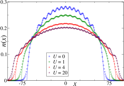
Figure 1: (Color online) DMRG data for the fermion density $n(x)$ in a harmonic trap with $N=30$ and $\omega^{2}=4\cdot 10^{-5}$ (points) compared to the analytical approximation in Eq. (12) (solid lines).

In Fig. 1 typical density distributions from DMRG are plotted for different $U$ in a trap with $N=30$ particles and $\omega^{2}=4\cdot 10^{-5}$, showing a localized fermion cloud with superimposed characteristic oscillations of different wavelengths. An analytical approximation to the data is also shown (solid lines), which will be derived in the following using bosonization and Bethe ansatz methods.

In order to understand the behavior of the density let us first consider the non-interacting case. In the continuous limit the wave-functions of the single-particle oscillator levels are given by $h_{n}(x)=\sqrt{\tfrac{1}{2^{n}n!}}\left(\tfrac{\omega}{\pi}\right)^{1/4}\,e^{-\omega x^{2}/2}\,H_{n}(\sqrt{\omega}x)$, where $H_{n}(x)$ denotes the $n$-th Hermite polynomial. The ground state density distribution at $U=0$ can be calculated as the sum over the filled Fermi sea of oscillator levels

$$n(x)=2\sum_{n=0}^{N/2-1}|h_{n}(x)|^{2}$$ (3)

for a system containing $N$ electrons. Using an expansion around the center of the trap, this function can be well described by a simple closed formula Gleisberg00 ; Butts97 ; Silvera81

$$n(x)\approx n_{0}(x)-\frac{(-1)^{N/2}}{\pi L_{\text{F}}}\frac{\cos\left(2k_{\text{F}}(x)x\right)}{1-x^{2}/L_{\text{F}}^{2}},$$ (4)

for $|x|\leq L_{F}$, where the density cloud is given by

$$n_{0}(x)=\frac{2\omega L_{F}}{\pi}\sqrt{1-x^{2}/L_{\text{F}}^{2}},$$ (5)

with a Thomas-Fermi size of $L_{F}=\sqrt{N/\omega}$ for $U=0$. The result in Eq. (4) resembles the corresponding expression for Friedel oscillations in a 1D box friedel , which also decay proportional to the reciprocal distance from the turning points $\pm L_{F}$. The slowly varying part of the density $n_{0}(x)$, Eq. (5), replaces the normally constant filling $n_{0}$. The period of the oscillations is related to the filling, so that the wavevector also becomes position dependent and is given by the non-local expression

$$2k_{\text{F}}(x)x = \pi\int_{0}^{x}n_{0}(y)\,dy$$

$$= \omega L_{F}\left[x\sqrt{1-x^{2}/L_{\text{F}}^{2}}+L_{F}\arcsin(x/L_{\text{F}})\right],$$

which follows from an expansion of the summed up oscillator wave-functions in Eq. (3). Note that the integration in Eq. (Density profile of interacting Fermions in a one-dimensional optical trap) is similar to the usual WKB approximation, where the local momentum $k(x)\approx\pi n(x)/2$ is integrated in space in order to predict the behavior in a changing potential. For constant filling the expression in Eq. (Density profile of interacting Fermions in a one-dimensional optical trap) reduces to the usual relation $k_{\text{F}}=\frac{\pi}{2}n_{0}$.

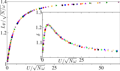
Figure 2: (Color online) The width $L_{\text{F}}(U)$ of the fermion cloud in the trap as determined from the local Bethe ansatz density as a function of the scaling variable $U/\sqrt{N\omega}$. The different symbols (colors) correspond to many different choices of $U\in[0,20]$, $\omega^{2}\in[10^{-5},16\times 10^{-5}]$ and $N\in[10,70]$. Inset: Effective exponent $\delta$ determined from a fit of $n_{0}^{\delta}(x)$ to the local Bethe ansatz density.

Before we analyze the oscillations in the presence of interactions, let us first consider the overall shape of the density cloud $n_{0}(x)$ for repulsive interactions $U>0$. For a translationally invariant 1D Hubbard model, the density is known as a function of $U$ and chemical potential $\mu$ from the non-trivial solution of the Bethe ansatz equations book . This is in sharp contrast to bosonic systems where the density is well described by a mean field approach, which can even be applied locally to non-uniform systems with the help of the Gross-Pitaevskii equation. One promising approach for the non-homogeneous fermion system may be to use the exact solution. In particular, if the external potential is slowly varying, the Bethe ansatz density for the chemical potential $\mu(x)=\mu_{0}+\omega^{2}x^{2}$ could be a good approximation for each location $x$ in the trap. Since strong long-range correlations exist, it is not a priori clear if such a local Bethe ansatz approximation with a translationally invariant system at each point is appropriate, but it agrees very well with our DMRG data for all $U$. This is especially surprising near the edges where the filling is low and also the discrete energy spectrum should play a role. At $U=0$ this approach corresponds to the density in Eq. (5). At $U\to\infty$ the interaction induces a Pauli principle between spin-up and down electrons, so that the system contains effectively twice $N=N_{\uparrow}+N_{\downarrow}$ non-interacting spin-incoherent particles, which results again in the density in Eq. (5), but with $L_{F}$ multiplied by a factor of $\sqrt{2}$. For intermediate $U$ the total size of the cloud therefore becomes interaction dependent with $\sqrt{N/\omega}\leq L_{F}(U)\leq\sqrt{2N/\omega}$. We find that the interaction dependence of the effective size $L_{F}(U)$ in fact follows a universal scaling behavior as a function of $U/\sqrt{N\omega}$ as shown in Fig. 2, which is related to the scaling behavior of the Bethe ansatz equations with $U/n_{0}$ at low filling $n_{0}$ book ; Soffing09 . The Bethe ansatz density at intermediate $U$ does not follow exactly the simple expression in Eq. (5), but can be approximated by the normalized shape if it is raised by a small exponent of $\delta\lesssim 1.3$ as shown in the inset in Fig. 2. It should be noted that Fig. 2 gives a quantitative estimate of the screening cloud for all interaction strengths $U$ and trap parameters as long as $N\omega\ll 1$.

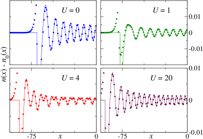
Figure 3: (Color online) Density oscillations around the slowly varying part $n_{0}(x)$ for $N=30$ and $\omega^{2}=4\cdot 10^{-5}$ compared to the analytical form in Eq. (12).

We can now subtract the Bethe ansatz estimate for the slowly-varying part of the density $n_{0}(x)$ from the DMRG data in order to analyze the oscillations as shown in Fig. 3. For weak interactions the Friedel-type oscillations in Eq. (4) can clearly be seen. At intermediate interactions $U=4$ two dominant wavevectors can be observed. At larger $U$ the faster oscillations dominate, corresponding to exactly one density maximum per particle, which is one typical signature of Wigner crystal oscillations. The oscillating signal is quite sensitive to the estimate of the uniform density, which has been subtracted. However, as can be seen in Fig. 3 the oscillations are symmetric in the entire trap without any visible bias towards positive or negative values, which shows that the local Bethe ansatz estimate works well.

A natural tool for calculating the density oscillations with the help of correlation functions in one-dimensional systems is bosonization Soffing09 . In the presence of a trapping potential, bosonization has been considered for interacting spinless fermions before Wonneberger01 ; Xianlong03 ; Artemenko04 ; Xianlong04 . For the spinful case we will now derive the central definitions of the bosonic creation and annihilation operators. Instead of the usual left- and right-moving bosons, only one bosonic field each for spin and charge ($\nu=\mathrm{c,s}$) is defined

$$\phi_{\nu}(u)=\phi_{\nu}^{0}+\frac{\hat{N}_{\uparrow}\pm\hat{N}_{\downarrow}}{\sqrt{2}}u+\sum_{n=1}^{\infty}\left(\tfrac{i}{\sqrt{n}}e^{-inu}b_{\nu,n}^{\phantom{\dagger}}+\text{h.c.}\right)$$ (7)

where the bosonic annihilation and creation operators

$$b^{\dagger}_{\nu,n}=\frac{1}{\sqrt{2n}}\sum_{m}(c_{\uparrow,m+n}^{\dagger}c_{\uparrow,m}^{\phantom{\dagger}}\pm c_{\downarrow,m+n}^{\dagger}c_{\downarrow,m}^{\phantom{\dagger}})$$ (8)

are expressed in terms of fermion operators $c_{\sigma,m}^{\dagger}$ of the $m$-th oscillator mode that are extended to include non-physical states $m<0$ (with $\pm$ corresponding to $\nu=\mathrm{c,s}$ respectively). The number operators $\hat{N}_{\uparrow}\pm\hat{N}_{\downarrow}$ are canonical conjugate to the zero modes $\phi_{\nu}^{0}$. The auxiliary variable $u\in[-\pi,\pi[$ should not be confused with the position $x$. Following the usual steps of the bosonization procedure egg07 , it is then easy to show that free-particle excitations relative to the Fermi edge are reproduced by the bosonic Hamiltonian

$$H=\hbar\omega\left(\sum_{\nu,n>0}nb_{\nu,n}^{\dagger}b_{\nu,n}^{\phantom{\dagger}}+(\hat{N}_{\uparrow}^{2}+\hat{N}_{\downarrow}^{2})/2\right)$$ (9)

The Fourier transformation of the oscillator levels defines a canonical auxiliary fermion field which can be bosonized as a vertex operator as usual

$$\tilde{\psi}^{\dagger}_{\sigma}(u)\equiv\frac{1}{\sqrt{2\pi}}\sum_{m}e^{imu}\,c_{\sigma,m}^{\dagger}\propto e^{-i(\phi_{c}(u)\pm\phi_{s}(u))/\sqrt{2}}.$$ (10)

The auxiliary field can in turn be used to give a non-local expression of the physical fermion fields in terms of the bosons

$$\psi^{\dagger}_{\sigma}(x) \equiv \sum_{n=0}^{\infty}h_{n}(x)\,c_{\sigma,n}^{\dagger}$$ (11)

$$= \frac{1}{\sqrt{2\pi}}\int_{-\pi}^{\pi}\,\sum_{n}h_{n}(x)\,e^{-inu}\tilde{\psi}^{\dagger}_{\sigma}(u){\,\mathrm{d}u}.$$

This expression can be made approximately local in $x$ by noticing that the wave-functions near the Fermi edge oscillate roughly as a function of $n$ with $h_{n}(x)\sim\cos(n\arccos(x/L_{F}))$. Therefore, $\psi^{\dagger}_{\sigma}(x)\sim e^{-i(\phi_{c}(u)\pm\phi_{s}(u))/\sqrt{2}}+e^{-i(\phi_{c}(-u)\pm\phi_{s}(-u))/\sqrt{2}}$ with $u\approx\arccos(x/L_{F})$, which also leads to densities in terms of derivatives of the boson field Wonneberger01 ; Xianlong03 ; Artemenko04 ; Xianlong04 . Without interactions this bosonization approximation is in fact more accurate than for translational invariant systems due to the linear oscillator spectrum. However, spinful interactions become quite complicated in the bosonized language, since general scattering terms appear that are not even momentum conserving.

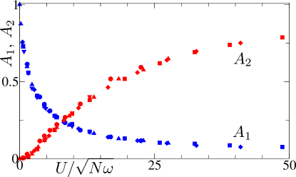
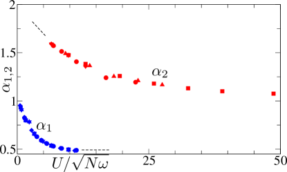
Figure 4: (Color online) Amplitudes $A_{1,2}$ (top) and exponents $\alpha_{1,2}$ (bottom) as determined by fitting Eq. (12) to DMRG data for different choices of $U$, $\omega$, and $N$.

Although we are not able to solve the system by a simple Bogoliubov transformation, the bosonization picture is useful since it is reasonable to expect that the leading instabilities are again a $2k_{F}$ Friedel and a $4k_{F}$ Wigner oscillation as for the translational invariant system schulz ; Soffing09 albeit with a changing wavevector along the trap according to Eq. (Density profile of interacting Fermions in a one-dimensional optical trap). We can therefore generalize Eq. (4) analogously to the Hubbard model with fixed boundary conditions and propose a general ansatz for the density in the trap for $|x|\leq L_{F}$

$$n(x)=n_{0}(x) - A_{1}\frac{(-1)^{N/2}}{\pi L_{\text{F}}}\frac{\cos\left(2k_{\text{F}}(x)\,x\right)}{[1-x^{2}/L_{F}^{2}]^{\alpha_{1}}}$$ (12)

$$- A_{2}\frac{1}{2\pi L_{\text{F}}}\frac{\cos\left(4k_{\text{F}}(x)\,x\right)}{[1-x^{2}/L_{F}^{2}]^{\alpha_{2}}},$$

where $L_{F}(U)$ is given in Fig. 2 and $k_{\text{F}}(x)$ is given in Eq. (Density profile of interacting Fermions in a one-dimensional optical trap) as a function of $L_{F}$. The amplitudes $A_{1,2}$ and the exponents $\alpha_{1,2}$ are unknown and have to be determined from fitting the DMRG data. As can be seen in Fig. 3 this formula fits the data extremely well even to within the last oscillation near the edge. In Fig. 4 the results for the amplitudes and the exponents are shown which again follow a scaling law as a function of $U/\sqrt{N\omega}$. For smaller amplitudes $A_{1,2}\lesssim 0.2$ the corresponding exponents in Fig. 4 could no longer be accurately determined. A clear increase of the faster Wigner-crystal oscillations $A_{2}$ can be seen with increasing $U$. At the same time the slower Friedel-type oscillations $A_{1}$ are suppressed. Both decay exponents generally decrease with increasing interactions which is qualitatively similar to the translational invariant Hubbard model book .

In conclusion we have analyzed the detailed behavior of the fermion density of the one-dimensional Hubbard model in a harmonic trap with the help of bosonization and the Bethe ansatz. The proposed analytical formula in Eq. (12) and the scaling behavior of the parameters in Fig. 2 and Fig. 4 provide very accurate predictions for the position dependent density $n(x)$ as a function of arbitrary interaction strengths $U$ and trap parameters in the limit $N\omega\ll 1$. Significant deviations can only be observed in the last oscillations near the edge of the density cloud. The overall density $n_{0}(x)$ follows a local Bethe ansatz approximation and the oscillations in the trap remain strong despite the lack of any hard-wall boundary conditions. A crossover from slower Friedel oscillations to faster Wigner crystal oscillations can be observed with increasing $U$. We hope that our results will be useful in the analysis of future experiments on ultracold fermions in a one-dimensional trap with local resolution. At the same time the good fit to the proposed analytical formula in Eq. (12) strongly suggests that the problem can be solved by further analyzing the bosonization formulas in Eqs. (7-11) in the presence of interactions, which might inspire future research on the topic.

We are thankful for useful discussions with I. Schneider and A. Struck. This work was supported by the DFG via the SFB/Transregio 49 and the MAINZ school of excellence.

References

- (1) I. Bloch, J. Dalibard, and W. Zwerger, Rev. Mod. Phys. 80, 885 (2008).
- (2) R. Jördens, et al., Nature 455, 204 (2008); U. Schneider, et al. Science 322, 1520 (2008).
- (3) J.F. Sherson, et al., Nature 467, 68 (2010).
- (4) T. Gericke, et al., Nature Phys. 4, 949 (2008).
- (5) J. Friedel, Il Nuovo Cimento 7, 287 (1958).
- (6) G.A. Fiete, et al., Phys. Rev. B 72, 045315 (2005); E.J. Mueller, Phys. Rev. B 72, 075322 (2005).
- (7) S.A. Söffing et al., Phys. Rev. B 79, 195114 (2009).
- (8) G. Bedürftig, B. Brendel, H. Frahm, and R.M. Noack, Phys. Rev. B 58, 10225 (1998).
- (9) S. Rommer and S. Eggert, Phys. Rev. B 62, 4370 (2000); F. Anfuso and S. Eggert, Phys. Rev. B 68, 241301 (2003); I. Schneider et al., Phys. Rev. Lett. 101, 206401 (2008).
- (10) S.R. White, I. Affleck, and D.J. Scalapino, Phys. Rev. B 65, 165122 (2002).
- (11) H.J. Schulz, Phys. Rev. Lett. 71, 1864 (1993)
- (12) D. Muth, M. Fleischhauer, and B. Schmidt, Phys. Rev. A 82, 013602 (2010).
- (13) M. Rigol, A. Muramatsu, G.G. Batrouni, and R.T. Scalettar, Phys. Rev. Lett. 91, 130403 (2003).
- (14) M. Rigol and A. Muramatsu, Phys. Rev. A 69, 053612 (2004).
- (15) G. Xianlong et al., Phys. Rev. B 73, 165120 (2006).
- (16) G. Xianlong and R. Asgari, Phys. Rev. A 77, 033604 (2008).
- (17) V.L. Campo and K. Capelle, Phys. Rev. A 72, 061602 (2005).
- (18) B. Schmidt et al., Phys. Rev. A 79, 063634 (2009)
- (19) A-Hai Chen and Gao Xianlong, Phys. Rev. A 81, 013628 (2010).
- (20) G.E. Astrakharchik, D. Blume, S. Giorgini, and L.P. Pitaevskii, Phys. Rev. Lett. 93, 050402 (2004); G. Xianlong, M. Polini, R. Asgari, and M.P. Tosi. Phys. Rev. A 73, 033609 (2006).
- (21) L. Kecke, H. Grabert, and W. Häusler, Phys. Rev. Lett. 94, 176802 (2005).
- (22) S.R. White, Phys. Rev. Lett. 69, 2863 (1992); Phys. Rev. B 48, 10345 (1993); U. Schollwöck, Rev. Mod. Phys. 77, 259 (2005).
- (23) F. Gleisberg, W. Wonneberger, U. Schloder, and C. Zimmermann, Phys. Rev. A 62, 063602 (2000).
- (24) D. A. Butts and D. S. Rokhsar, Phys. Rev. A 55, 4346 (1997).
- (25) I. F. Silvera and J. T. M. Walraven, Journal of Applied Physics 52, 2304 (1981).
- (26) The One-Dimensional Hubbard Model by F.H.L. Essler, et al., (Cambridge University Press, Cambridge, 2005).
- (27) W. Wonneberger, Phys. Rev. A 63, 063607 (2001).
- (28) G. Xianlong, F. Gleisberg, F. Lochmann, and W. Wonneberger, Phys. Rev. A 67, 023610 (2003).
- (29) S. N. Artemenko, G. Xianlong, and W. Wonneberger, J. Phys. B: Atomic, Molecular and Optical Physics 37, S49 (2004).
- (30) G. Xianlong and W. Wonneberger, J. Phys. B: Atomic, Molecular and Optical Physics 37, 2363 (2004).
- (31) For a review see S. Eggert, Theoretical Survey of One Dimensional Wire Systems, edited by Y. Kuk, et al., (Sowha Publishing, Seoul, 2007), p. 13; arXiv:0708.0003.