2 Institute for High Energy Physics, IHEP, Pobeda 1, 142281 Protvino, Russia
3 School of Physics and Astronomy, University of Edinburgh, JCMB, KB, Mayfield Rd, Edinburgh EH9 3JZ, Scotland
4 Physikalisches Institut, Albert-Ludwigs-Universität Freiburg, Hermann-Herder-Straße 3, D-79104 Freiburg i. B., Germany
5 NIKHEF, Science Park, Amsterdam, The Netherlands
6 Department of Physics and Astronomy, University College, London, WC1E 6BT, UK
7 Departament d’Estructura i Constituents de la Matèria, Universitat de Barcelona, Diagonal 647, E-08028 Barcelona, Spain
8 Department of Physics, Oxford University, Denys Wilkinson Bldg, Keble Rd, Oxford, OX1 3RH, UK
9 CERN, CH–1211 Genève 23, Switzerland; Antwerp University, B–2610 Wilrijk, Belgium; University of California Davis, CA, USA
10 CEA, DSM/IRFU, CE-Saclay, Gif-sur-Yvetee, France
11 Dipartimento di Fisica, Università di Milano and INFN, Sezione di Milano, Via Celoria 16, I-20133 Milano, Italy
12 Deutsches Elektronensynchrotron DESY Notkestraße 85 D–22607 Hamburg, Germany
13 Physics and Astronomy Department, Michigan State University, East Lansing, MI 48824, USA
14 Institut für Theoretische Physik, Universität Zürich, CH-8057 Zürich, Switzerland
15 Taipei Municipal University of Education, Taipei, Taiwan
16 School of Physics, University College Dublin Science Centre North, UCD Belfeld, Dublin 4, Ireland
17 Department of Physics, Southern Methodist University, Dallas, TX 75275-0175, USA
18 Physikalisches Institut, Universität Heidelberg Philosophenweg 12, D–69120 Heidelberg, Germany
19 Department of Astronomy and Theoretical Physics, Lund University, Sölvegatan 14A, S-223 62 Lund, Sweden
20 Cavendish Laboratory, University of Cambridge, CB3 OHE, UK
21 Institut für Theoretische Teilchenhysik und Kosmologie, RWTH Aachen University, D-52056 Aachen, Germany
22 Theory Group, Physics Department, CERN, CH-1211 Geneva 23, Switzerland
The PDF4LHC Working Group Interim Report
Abstract
This document is intended as a study of benchmark cross sections at the LHC (at 7 TeV) at NLO using modern PDFs currently available from the 6 PDF fitting groups that have participated in this exercise. It also contains a succinct user guide to the computation of PDFs, uncertainties and correlations using available PDF sets.
A companion note provides an interim summary of the current recommendations of the PDF4LHC working group for the use of parton distribution functions (PDFs) and of PDF uncertainties at the LHC, for cross section and cross section uncertainty calculations.
1 Introduction
The LHC experiments are currently producing cross sections from the 7 TeV data, and thus need accurate predictions for these cross sections and their uncertainties at NLO and NNLO. Crucial to the predictions and their uncertainties are the parton distribution functions (PDFs) obtained from global fits to data from deep-inelastic scattering, Drell-Yan and jet data. A number of groups have produced publicly available PDFs using different data sets and analysis frameworks. It is one of the charges of the PDF4LHC working group to evaluate and understand differences among the PDF sets to be used at the LHC, and to provide a protocol for both experimentalists and theorists to use the PDF sets to calculate central cross sections at the LHC, as well as to estimate their PDF uncertainty. This current note is intended to be an interim summary of our level of understanding of NLO predictions as the first LHC cross sections at 7 TeV are being produced 111Comparisons at NNLO for , and Higgs production can be found in ref. [1]. The intention is to modify this note as improvements in data/understanding warrant.
For the purpose of increasing our quantitative understanding of the similarities and differences between available PDF determinations, a benchmarking exercise between the different groups was performed. This exercise was very instructive in understanding many differences in the PDF analyses: different input data, different methodologies and criteria for determining uncertainties, different ways of parametrizing PDFs, different number of parametrized PDFs, different treatments of heavy quarks, different perturbative orders, different ways of treating (as an input or as a fit parameter), different values of physical parameters such as itself and heavy quark masses, and more. This exercise was also very instructive in understanding where the PDFs agree and where they disagree: it established a broad agreement of PDFs (and uncertainties) obtained from data sets of comparable size and it singled out relevant instances of disagreement and of dependence of the results on assumptions or methodology.
The outline of this interim report is as follows. The first three sections are devoted to a description of current PDF sets and their usage. In Sect. 2 we present several modern PDF determinations, with special regard to the way PDF uncertainties are determined. First we summarize the main features of various sets, then we provide an explicit users’ guide for the computation of PDF uncertainties. In Sect. 3 we discuss theoretical uncertainties on PDFs. We first introduce various theoretical uncertainties, then we focus on the uncertainty related to the strong coupling and also in this case we give both a presentation of choices made by different groups and a users’ guide for the computation of combined PDF+ uncertainties. Finally in Sect. 4 we discuss PDF correlations and the way they can be computed.
2 PDF determinations - experimental uncertainties
Experimental uncertainties of PDFs determined in global fits (usually called “PDF uncertainties” for short) reflect three aspects of the analysis, and differ because of different choices made in each of these aspects: (1) the choice of data set; (2) the type of uncertainty estimator used which is used to determine the uncertainties and which also determines the way in which PDFs are delivered to the user; (3) the form and size of parton parametrization. First, we briefly discuss the available options for each of these aspects (at least, those which have been explored by the various groups discussed here) and summarize the choices made by each group; then, we provide a concise user guide for the determination of PDF uncertainties for available fits. We will in particular discuss the following PDF sets (when several releases are available the most recent published ones are given in parenthesis in each case): ABKM/ABM [2, 3], CTEQ/CT (CTEQ6.6 [4], CT10 [5]), GJR [6, 7], HERAPDF (HERAPDF1.0 [8]), MSTW (MSTW08 [9]), NNPDF (NNPDF2.0 [10]). There is a significant time-lag between the development of a new PDF and the wide adoption of its use by experimental collaborations, so in some cases, we report not on the most up-to-date PDF from a particular group, but instead on the most widely-used.
2.1 Features, tradeoffs and choices
2.1.1 Data Set
There is a clear tradeoff between the size and the consistency of a data set: a wider data set contains more information, but data coming from different experiment may be inconsistent to some extent. The choices made by the various groups are the following:
-
•
The CTEQ, MSTW and NNPDF data sets considered here include both electroproduction and hadroproduction data, in each case both from fixed-target and collider experiments. The electroproduction data include electron, muon and neutrino deep–inelastic scattering data (both inclusive and charm production). The hadroproduction data include Drell-Yan (fixed target virtual photon and collider and production) and jet production 222Although the comparisons included in this note are only at NLO,we note that, to date, the inclusive jet cross section, unlike the other processes in the list above, has been calculated only to NLO, and not to NNLO. This may have an impact on the precision of NNLO global PDF fits that include inclusive jet data..
-
•
The GJR data set includes electroproduction data from fixed-target and collider experiments, and a smaller set of hadroproduction data. The electroproduction data include electron and muon inclusive deep–inelastic scattering data, and deep-inelastic charm production from charged leptons and neutrinos. The hadroproduction data includes fixed–target virtual photon Drell-Yan production and Tevatron jet production.
-
•
The ABKM/ABM data sets include electroproduction from fixed-target and collider experiments, and fixed–target hadroproduction data. The electroproduction data include electron, muon and neutrino deep–inelastic scattering data (both inclusive and charm production). The hadroproduction data include fixed–target virtual photon Drell-Yan production. The most recent version, ABM10 [11], includes Tevatron jet data.
-
•
The HERAPDF data set includes all HERA deep-inelastic inclusive data.
2.1.2 Statistical treatment
Available PDF determinations fall in two broad categories: those based on a Hessian approach and those which use a Monte Carlo approach. The delivery of PDFs is different in each case and will be discussed in Sect. 2.2.
Within the Hessian method, PDFs are determined by minimizing a suitable log-likelihood function. Different groups may use somewhat different definitions of , for example, by including entirely, or only partially, correlated systematic uncertainties. While some groups account for correlated uncertainties by means of a covariance matrix, other groups treat some correlated systematics (specifically but not exclusively normalization uncertanties) as a shift of data, with a penalty term proportional to some power of the shift parameter added to the . The reader is referred to the original papers for the precise definition adopted by each group, but it should be born in mind that because of all these differences, values of the quoted by different groups are in general only roughly comparable.
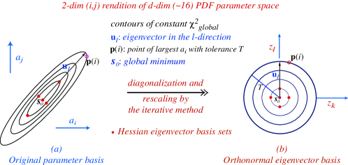
With the covariance matrix approach, we can define , are data, theoretical predictions, is the number of data points (note the inclusion of the factor in the definition) and is the covariance matrix. Different groups may use somewhat different definitions of the covariance matrix, by including entirely or only partially correlated uncertainties. The best fit is the point in parameter space at which is minimum, while PDF uncertainties are found by diagonalizing the (Hessian) matrix of second derivatives of the at the minimum (see Fig. 1) and then determining the range of each orthonormal Hessian eigenvector which corresponds to a prescribed increase of the function with respect to the minimum.
In principle, the variation of the which corresponds to a 68% confidence (one sigma) is . However, a larger variation , with a suitable “tolerance” parameter [12, 13, 14] may turn out to be necessary for more realistic error estimates for fits containing a wide variety of input processes/data, and in particular in order for each individual experiment which enters the global fit to be consistent with the global best fit to one sigma (or some other desired confidence level such as 90%). Possible reasons why this is necessary could be related to data inconsistencies or incompatibilities, underestimated experimental systematics, insufficiently flexible parton parametrizations, theoretical uncertainties or approximation in the PDF extraction. At present, HERAPDF and ABKM use , GJR uses at one sigma (corresponding to at 90% c.l.), CTEQ6.6 uses at 90% c.l. (corresponding to to one sigma) and MSTW08 uses a dynamical tolerance [9], i.e. a different value of for each eigenvector, with values for one sigma ranging from to and most values being .
Within the NNPDF method, PDFs are determined by first producing a Monte Carlo sample of pseudo-data replicas. Each replica contains a number of points equal to the number of original data points. The sample is constructed in such a way that, in the limit , the central value of the -th data point is equal to the mean over the values that the -th point takes in each replica, the uncertainty of the same point is equal to the variance over the replicas, and the correlations between any two original data points is equal to their covariance over the replicas. From each data replica, a PDF replica is constructed by minimizing a function. PDF central values, uncertainties and correlations are then computed by taking means, variances and covariances over this replica sample. NNPDF uses a Monte Carlo method, with each PDF replica obtained as the minimum which satisfies a cross-validation criterion [15, 10], and is thus larger than the absolute minimum of the . This method has been used in all NNPDF sets from NNPDF1.0 onwards.
2.1.3 Parton parametrization
Existing parton parametrizations differ in the number of PDFs which are independently parametrized and in the functional form and number of independent parameters used. They also differ in the choice of individual linear combinations of PDFs which are parametrized. In what concerns the functional form, the most common choice is that each PDF at some reference scale is parametrized as
| (1) |
where is a function which tends to a constant both for and , such as for instance (HERAPDF). The fit parameters are , and the parameters in . Some of these parameters may be chosen to take a fixed value (including zero). The general form Eq. (1) is adopted in all PDF sets which we discuss here except NNPDF, which instead lets
| (2) |
where is a neural network, and is is a “preprocessing” function. The fit parameters are the parameters which determine the shape of the neural network (a 2-5-3-1 feed-forward neural network for NNPDF2.0). The preprocessing function is not fitted, but rather chosen randomly in a space of functions of the general form Eq. (2) within some acceptable range of the parameters and , and with .
The basis functions and number of parameters are the following.
-
•
ABKM parametrizes the two lightest flavours and antiflavours, the total strangeness and the gluon (five independent PDFs) with 21 free parameters.
-
•
CTEQ6.6 and CT10 parametrize the two lightest flavours and antiflavours the total strangeness and the gluon (six independent PDFs) with respectively 22 and 26 free parameters.
-
•
GJR parametrizes the two lightest flavours and antiflavours and the gluon with 20 free parameters (five independent PDFs); the strange distribution is assumed to be either proportional to the light sea or to vanish at a low scale GeV at which PDFs become valence-like.
-
•
HERAPDF parametrizes the two lightest flavours, , the combination and the gluon with 10 free parameters (six independent PDFs), strangeness is assumed to be proportional to the distribution; HERAPDF also studies the effect of varying the form of the parametrization and of and varying the relative size of the strange component and thus determine a model and parametrization uncertainty (see Sect.3.2.3 for more details).
-
•
MSTW parametrizes the three lightest flavours and antiflavours and the gluon with 28 free parameters (seven independent PDFs) to find the best fit, but 8 are held fixed in determining uncertainty eigenvectors.
-
•
NNPDF parametrizes the three lightest flavours and antiflavours and the gluon with 259 free parameters (37 for each of the seven independent PDFs).
2.2 PDF delivery and usage
The way uncertainties should be determined for a given PDF set depends on whether it is a Monte Carlo set (NNPDF) or a Hessian set (all other sets). We now describe the procedure to be followed in each case.
2.2.1 Computation of Hessian PDF uncertainties
For Hessian PDF sets, both a central set and error sets are given. The number of eigenvectors is equal to the number of free parameters. Thus, the number of error PDFs is equal to twice that. Each error set corresponds to moving by the specified confidence level (one sigma or 90% c.l.) in the positive or negative direction of each independent orthonormal Hessian eigenvector.
Consider a variable ; its value using the central PDF for an error set is given by . is the value of that variable using the PDF corresponding to the “” direction for the eigenvector , and the value for the variable using the PDF corresponding to the “” direction.
| (3) |
adds in quadrature the PDF error contributions that lead to an increase in the observable , and the PDF error contributions that lead to a decrease. The addition in quadrature is justified by the eigenvectors forming an orthonormal basis. The sum is over all eigenvector directions. Ordinarily, one of and will be positive and one will be negative, and thus it is trivial as to which term is to be included in each quadratic sum. For the higher number (less well-determined) eigenvectors, however, the “” and “”eigenvector contributions may be in the same direction. In this case, only the more positive term will be included in the calculation of and the more negative in the calculation of [24]. Thus, there may be less than non-zero terms for either the “” or “” directions. A symmetric version of this is also used by many groups, given by the equation below:
In most cases, the symmetric and asymmetric forms give very similar results. The extent to which the symmetric and asymmetric errors do not agree is an indication of the deviation of the distribution from a quadratic form. The lower number eigenvectors, corresponding to the best known directions in eigenvector space, tend to have very symmetric errors, while the higher number eigenvectors can have asymmetric errors. The uncertainty for a particular observable then will (will not) tend to have a quadratic form if it is most sensitive to lower number (higher number) eigenvectors. Deviations from a quadratic form are expected to be greater for larger excursions, i.e. for 90%c.l. limits than for 68% c.l. limits.
The HERAPDF analysis also works with the Hessian matrix, defining experimental error PDFs in an orthonormal basis as described above. The symmetric formula Eq. LABEL:eq:symm is most often used to calculate the experimental error bands on any variable, but it is possible to use the asymmetric formula as for MSTW and CTEQ. (For HERAPDF1.0 these errors are provided at c.l. in the LHAPDF file: HERAPDF10 EIG.LHgrid).
Other methods of calculating the PDF uncertainties independent of the Hessian method, such as the Lagrange Multiplier approach [12], are not discussed here.
2.2.2 Computation of Monte Carlo PDF uncertainties
For the NNPDF Monte Carlo set, a Monte Carlo sample of PDFs is given. The expectation value of any observable (for example a cross–section) which depends on the PDFs is computed as an average over the ensemble of PDF replicas, using the following master formula:
| (5) |
where is the number of replicas of PDFs in the Monte Carlo ensemble. The associated uncertainty is found as the standard deviation of the sample, according to the usual formula
| (6) | |||||
These formulae may also be used for the determination of central values and uncertainties of the parton distribution themselves, in which case the functional is identified with the parton distribution : . Indeed, the central value for PDFs themselves is given by
| (7) |
NNPDF provides both sets of and replicas. The larger set ensures that statistical fluctuations are suppressed so that even oddly-shaped probability distributions such as non-gaussian or asymmetric ones are well reproduced, and more detailed features of the probability distributions such as correlation coefficients or uncertainties on uncertainties can be determined accurately. However, for most common applications such as the determination of the uncertainty on a cross section the smaller replica set is adequate, and in fact central values can be determined accurately using a yet smaller number of PDFs (typically ), with the full set of only needed for the reliable determination of uncertainties.
NNPDF also provides a set 0 in the NNPDF20_100.LHgrid LHAPDF file, as in previous releases of the NNPDF family, while replicas 1 to 100 correspond to PDF sets 1 to 100 in the same file. This set 0 contains the average of the PDFs, determined using Eq. (7): in other words, set 0 contains the central NNPDF prediction for each PDF. This central prediction can be used to get a quick evaluation of a central value. However, it should be noticed that for any which depends nonlinearly on the PDFs, . This means that a cross section evaluated from the central set is not exactly equal to the central cross section (though it will be for example for deep-inelastic structure functions, which are linear in the PDFs). Hence, use of the 0 set is not recommended for precision applications, though in most cases it will provide a good approximation. Note that set should not be included when computing an average with Eq. (5), because it is itself already an average.
Equation (6) provides the 1–sigma PDF uncertainty on a general quantity which depends on PDFs. However, an important advantage of the Monte Carlo method is that one does not have to rely on a Gaussian assumption or on linear error propagation. As a consequence, one may determine directly a confidence level: e.g. a 68% c.l. for is simply found by computing the values of and discarding the upper and lower 16% values. In a general non-gaussian case this 68% c.l. might be asymmetric and not equal to the variance (one–sigma uncertainty). For the observables of the present benchmark study the 1–sigma and 68% c.l. PDF uncertainties turn out to be very similar and thus only the former are given, but this is not necessarily the case in in general. For example, the one sigma error band on the NNPDF2.0 large gluon and the small strangeness is much larger than the corresponding 68% CL band, suggesting non-gaussian behavior of the probability distribution in these regions, in which PDFs are being extrapolated beyond the data region.
3 PDF determinations - Theoretical uncertainties
Theoretical uncertainties of PDFs determined in global fits reflect the approximations in the theory which is used in order to relate PDFs to measurable quantities. The study of theoretical PDF uncertainties is currently less advanced that that of experimental uncertainties, and only some theoretical uncertainties have been explored. One might expect that the main theoretical uncertainties in PDF determination should be related to the treatment of the strong interaction: in particular to the values of the QCD parameters, specifically the value of the strong coupling and of the quark masses and and uncertainties related to the truncation of the perturbative expansion (commonly estimated through the variation of renormalization and factorization scales). Further uncertainties are related to the treatment of heavy quark thresholds, which are handled in various ways by different groups (fixed flavour number vs. variable flavour number schemes, and in the latter case different implementations of the variable flavour number scheme), and to further approximations such as the use of -factor approximations. Finally, more uncertainties may be related to weak interaction parameters (such as the mass) and to the treatment of electroweak effects (such as QED PDF evolution [16] ).
Of these uncertainties, the only one which has been explored systematically by the majority of the PDF groups is the uncertainty. The way uncertainty can be determined using CTEQ, HERAPDF, MSTW, and NNPDF will be discussed in detail below. HERAPDF also provides model and parametrization uncertainties which include the effect of varying and , as well as the effect of varying the parton parametrization, as will also be discussed below. Sets with varying quark masses and their implications have recently been made available by MSTW [17], the effects of varying and have been included by ABKM [2] and preliminary studies of the effect of and have also been presented by NNPDF [18]. Uncertainties related to factorization and renormalization scale variation and to electroweak effects are so far not available. For the benchmarking exercise of Sec. 5, results are given adopting common values of electroweak parameters, and at least one common value of (though values for other values of are also given), but no attempt has yet been made to benchmark the other aspects mentioned above.
3.1 The value of and its uncertainty
We thus turn to the only theoretical uncertainty which has been studied systematically so far, namely the uncertainty on . The choice of value of is clearly important because it is strongly correlated to PDFs, especially the gluon distribution (the correlation of with the gluon distribution using CTEQ, MSTW and NNPDF PDFs is studied in detail in Ref. [19]). See also Ref. [2] for a discussion of this correlation in the ABKM PDFs. There are two separate issues related to the value of in PDF fits: first, the choice of for which PDFs are made available, and second the choice of the preferred value of to be used when giving PDFs and their uncertainties. The two issues are related but independent, and for each of the two issue two different basic philosophies may be adopted.
Concerning the range of available values of :
-
•
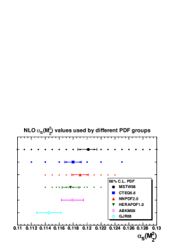
PDFs fits are performed for a number of different values of . Though a PDF set corresponding to some reference value of is given, the user is free to choose any of the given sets. This approach is adopted by CTEQ (0.118), HERAPDF (0.1176), MSTW (0.120) and NNPDF (0.119), where we have denoted in parenthesis the reference (NLO) value of for each set.
-
•
is treated as a fit parameters and PDFs are given only for the best–fit value. This approach is adopted by ABKM (0.1179) and GJR (0.1145), where in parenthesis the best-fit (NLO) value of is given.
Concerning the preferred central value and the treatment of the uncertainty:
-
•
The value of is taken as an external parameter, along with other parameters of the fit such as heavy quark masses or electroweak parameter. This approach is adopted by CTEQ, HERAPDF1.0 and NNPDF. In this case, there is no apriori central value of and the uncertainty on is treated by repeating the PDF determination as is varied in a suitable range. Though a range of variation is usually chosen by the groups, any other range may be chosen by the user.
-
•
The value of is treated as a fit parameter, and it is determined along with the PDFs. This approach is adopted by MSTW, ABKM and GJR08. In the last two cases, the uncertainty on is part of the Hessian matrix of the fit. The MSTW approach is explained below.
As a cross-check,CTEQ [20] has also used the world average value of as an additional input to the global fit.
The values of for which fits are available, as well as the default values and uncertainties used by each group are summarized in Fig. 2 333There is implicitly an additional uncertainty due to scale variation.See for example Ref. [26].. The most recent world average value of is [22] 444We note that the values used in the average are from extractions at different orders in the perturbative expansion.. However, a more conservative estimate of the uncertainty on was felt to be appropriate for the benchmarking exercise summarized in this note, for which we have taken at 90%c.l. (corresponding to 0.0012 at one sigma). This uncertainty has been used for the CTEQ, NNPDF and HERAPDF studies. For MSTW, ABKM and GJR the preferred uncertainty for each group is used, though for MSTW in particular this is close to 0.0012 at one sigma. It may not be unreasonable to argue that a yet larger uncertainty may be appropriate.
When comparing results obtained using different PDF sets it should be borne in mind that if different values of are used, cross section predictions change both because of the dependence of the cross section on the value of (which for some processes such as top production or Higgs production in gluon-gluon fusion may be quite strong), and because of the dependence of the PDFs themselves on the value of . Differences due to the PDFs alone can be isolated only when performing comparisons at a common value of .
3.2 Computation of PDF+ uncertainties
Within the quadratic approximation to the dependence of on parameters (i.e. linear error propagation), it turns out that even if PDF uncertainty and the uncertainty are correlated, the total one-sigma combined PDF+ uncertainty including this correlation can be simply found without approximation by computing the one sigma PDF uncertainty with fixed at its central value and the one-sigma uncertainty with the PDFs fixed their central value, and adding results in quadrature [20], and similarly for any other desired confidence level.
For example, if is the PDF uncertainty for a cross section and is the uncertainty, the combined uncertainty is
| (8) |
Other treatments can be used when deviations from the quadratic approximation are possible. Indeed,for MSTW because of the use of dynamical tolerance linear error propagation does not necessarily apply. For NNPDF, because of the use of a Monte Carlo method linear error propagation is not assumed: in practice, addition in quadrature turns out to be a very good approximation, but an exact treatment is computationally simpler. We now describe in detail the procedure for the computation of and PDF uncertainties (and for HERAPDF also of model and parametrization uncertainties) for various parton sets.
3.2.1 CTEQ - Combined PDF and uncertainties
CTEQ takes as an external input parameter and provides the CTEQ6.6alphas [20] (or the CT10alpha [5]) series which contains 4 sets extracted using ; The uncertainty associated with can be evaluated by computing any given observable with in the partonic cross-section and with the PDF sets that have been extracted with these values of . The differences
| (9) |
are the uncertainties according to CTEQ. In [20] it has been demonstrated that, in the Hessian approach, the combination in quadrature of PDF and uncertainties is correct within the quadratic approximation. In the studies in Ref. [20], CTEQ did not find appreciable deviations from the quadratic approximation, and thus the procedure described below will be accurate for the cross sections considered here.
Therefore, for CTEQ6.6 the combined PDF+uncertainty is given by
| (10) | |||||
3.2.2 MSTW - Combined PDF and uncertainties
MSTW fits together with the PDFs and obtains and . Any correlation between the PDF and the uncertainties is taken into account with the following recipe [23]. Beside the best-fit sets of PDFs, which correspond to , four more sets,both at NLO and at NNLO, of PDFs are provided. The latter are extracted setting as input , where is the standard deviation indicated here above. Each of these extra sets contains the full parametrization to describe the PDF uncertainty. Comparing the results of the five sets, the combined PDF+uncertainty is defined as:
| (11) | |||||
where run over the five values of under study, and the corresponding PDF uncertainties are used.
The central and , where sets are all obtained using the dynamical tolerance prescription for PDF uncertainty which determines the uncertainty when the quality of the fit to any one data set (relative to the best fit for the preferred value of ) becomes sufficiently poor. Naively one might expect that the PDF uncertainty for the might then be zero since one is by definition already at the limit of allowed fit quality for one data set. If this were the case the procedure of adding PDF and uncertainties would be a very good approximation. However, in practice there is freedom to move the PDFs in particular directions without the data set at its limit of fit quality becoming worse fit, and some variations can be quite large before any data set becomes sufficiently badly fit for the criterion for uncertainty to be met. This can led to significantly larger PDF uncertainties than the simple quadratic prescription. In particular, since there is a tendency for the best fit to have a too low value of at low , at higher value the small- gluon has freedom to increase without spoiling the fit, and the PDF uncertainty is large in the upwards direction for Higgs production.
3.2.3 HERAPDF - , model and parametrization uncertainties
HERAPDF provides not only uncertainties, but also model and parametrization uncertainties. Note that at least in part parametrization uncertainty will be accounted for by other groups by the use of a significantly larger number of initial parameters, the use of a large tolerance (CTEQ, MSTW) or by a more general parametrization (NNPDF), as discussed in Sect. 2.1.3. However, model uncertainties related to heavy quark masses are not determined by other groups.
The model errors come from variation of the choices of: charm mass (GeV); beauty mass ( GeV); minimum of data used in the fit ( GeV2); fraction of strange sea in total d-type sea ( at the starting scale). The model errors are calculated by taking the difference between the central fit and the model variation and adding them in quadrature, separately for positive and negative deviations. (For HERAPDF1.0 the model variations are provided as members 1 to 8 of the LHAPDF file: HERAPDF10 VAR.LHgrid).
The parametrization errors come from: variation of the starting scale GeV2; variations of the basic 10 parameter fit to 11 parameter fits in which an extra parameter is allowed to be free for each fitted parton distribution. In practice only three of these extra parameter variations have significantly different PDF shapes from the central fit. The parametrization errors are calculated by storing the difference between the parametrization variant and the central fit and constructing an envelope representing the maximal deviation at each value. (For HERAPDF1.0 the parametrization variations are provided as members 9 to 13 of the LHAPDF file: HERAPDF10 VAR.LHgrid).
HERAPDF also provide an estimate of the additional error due to the uncertainty on . Fits are made with the central value, , varied by . The c.l. error on any variable should be calculated by adding in quadrature the difference between its value as calculated using the central fit and its value using these two alternative values; c.l. values may be obtained by scaling the result down by 1.645. (For HERAPDF1.0 these variations are provided as members 9,10,11 of the LHAPDF file: HERAPDF10 ALPHAS.LHgrid for , respectively). Additionally members 1 to 8 provide PDFs for values of ranging from 0.114 to 0.122). The total PDF + uncertainty for HERAPDF should be constructed by adding in quadrature experimental, model, parametrization and uncertainties.
3.2.4 NNPDF - Combined PDF and uncertainties
For the NNPDF2.0 family, PDF sets obtained with values of in the range from 0.114 to 0.124 in steps of are available in LHAPDF. Each of these sets is denoted by NNPDF20_as_0114_100.LHgrid, NNPDF20_as_0115_100.LHgrid, … and has the same structure as the central NNPDF20_100.LHgrid set: PDF set number 0 is the average PDF set, as discussed above
| (12) |
for the different values of , while sets from 1 to 100 are the 100 PDF replicas corresponding to this particular value of . Note that in general not only the PDF central values but also the PDF uncertainties will depend on .
The methodology used within the NNPDF approach to combine PDF and uncertainties is discussed in Ref. [19, 28]. One possibility is to add in quadrature the PDF and uncertainties, using PDFs obtained from different values of , which as discussed above is correct in the quadratic approximation. However use of the exact correlated Monte Carlo formula turns out to be actually simpler, as we now show.
If the sum in quadrature is adopted, for a generic cross section which depends on the PDFs and the strong coupling , we have
| (13) |
where PDF(±) stands schematically for the PDFs obtained when is varied within its 1–sigma range, . The PDF+ uncertainty is
| (14) |
with the PDF uncertainty on the observable computed from the set with the central value of .
The exact Monte Carlo expression instead is found noting that the average over Monte Carlo replicas of a general quantity which depends on both and the PDFs, is
| (15) |
where stands for the replica of the PDF fit obtained using as the value of the strong coupling; is the total number of PDF replicas
| (16) |
and is the number of PDF replicas for each value of . If we assume that is gaussianly distributed about its central value with width equal to the stated uncertainty, the number of replicas for each different value of is
| (17) |
with and the assumed central value and 1–sigma uncertainty of . Clearly with a Monte Carlo method a different probability distribution of values could also be assumed. For example, if we assume and we take nine distinct values , assuming 100 replicas for the central value () we get .
The combined PDF+ uncertainty is then simply found by using Eq. (6) with averages computed using Eq. (15). The difference between Eq. (15) and Eq. (14) measures deviations from linear error propagation. The NNPDF benchmark results presented below are obtained using Eq. (15) with at one sigma. No significant deviations from linear error propagation were observed.
It is interesting to observe that the same method can be used to determine the combined uncertainty of PDFs and other physical parameters, such as heavy quark masses.
4 PDF correlations
The uncertainty analysis may be extended to define a correlation between the uncertainties of two variables, say and As for the case of PDFs, the physical concept of PDF correlations can be determined both from PDF determinations based on the Hessian approach and on the Monte Carlo approach.
4.1 PDF correlations in the Hessian approach
Consider the projection of the tolerance hypersphere onto a circle of radius 1 in the plane of the gradients and in the parton parameter space [13, 24]. The circle maps onto an ellipse in the plane. This “tolerance ellipse” is described by Lissajous-style parametric equations,
| (18) | |||||
| (19) |
where the parameter varies between 0 and , and . and are the maximal variations and evaluated according to the Equation, and is the angle between and in the space, with
| (20) |
The quantity characterizes whether the PDF degrees of freedom of and are correlated (), anti-correlated (), or uncorrelated (). If units for and are rescaled so that (e.g., ), the semimajor axis of the tolerance ellipse is directed at an angle (or with respect to the axis for (or ). In these units, the ellipse reduces to a line for and becomes a circle for , as illustrated by Fig. 3. These properties can be found by diagonalizing the equation for the correlation ellipse. Its semiminor and semimajor axes (normalized to ) are
| (21) |
The eccentricity is therefore approximately equal to as .
| (22) |
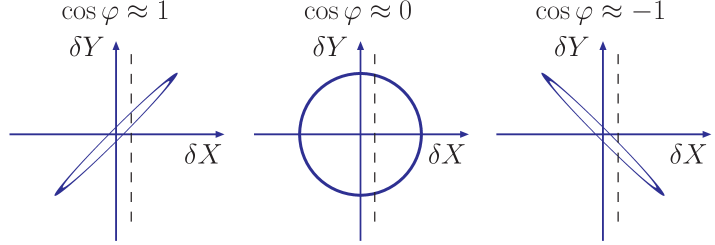
A magnitude of close to unity suggests that a precise measurement of (constraining to be along the dashed line in Fig. 3) is likely to constrain tangibly the uncertainty in , as the value of shall lie within the needle-shaped error ellipse. Conversely, implies that the measurement of is not likely to constrain strongly.555The allowed range of for a given is where
The values of and are also sufficient to estimate the PDF uncertainty of any function of and by relating the gradient of to and via the chain rule:
| (23) |
Of particular interest is the case of a rational function pertinent to computations of various cross section ratios, cross section asymmetries, and statistical significance for finding signal events over background processes [24]. For rational functions Eq. (23) takes the form
| (24) |
For example, consider a simple ratio, . Then is suppressed () if and are strongly correlated, and it is enhanced () if and are strongly anticorrelated.
As would be true for any estimate provided by the Hessian method, the correlation angle is inherently approximate. Eq. (20) is derived under a number of simplifying assumptions, notably in the quadratic approximation for the function within the tolerance hypersphere, and by using a symmetric finite-difference formula for that may fail if is not monotonic. With these limitations in mind, we find the correlation angle to be a convenient measure of interdependence between quantities of diverse nature, such as physical cross sections and parton distributions themselves. For example, in Section 5.2.2, the correlations for the benchmark cross sections are given with respect to that for production. As expected, the and cross sections are very correlated with that for the , while the Higgs cross sections are uncorrelated (=120 GeV) or anti-correlated (=240 GeV). Thus, the PDF uncertainty for the ratio of the cross section for a 240 GeV Higgs boson to that of the cross section for boson production is larger than the PDF uncertainty for Higgs boson production by itself.
A simple code (corr.C) is available from the PDF4LHC website that calculates the correlation cosine between any two observables given two text files that present the cross sections for each observable as a function of the error PDFs.
4.2 PDF correlations in the Monte Carlo approach
General correlations between PDFs and physical observables can be computed within the Monte Carlo approach used by NNPDF using standard textbook methods. To illustrate this point, let us compute the the correlation coefficient for two observables and which depend on PDFs (or are PDFs themselves). This correlation coefficient in the Monte Carlo approach is given by
| (25) |
where the averages are taken over ensemble of the values of the observables computed with the different replicas in the NNPDF2.0 set, and are the standard deviations of the ensembles. The quantity characterizes whether two observables (or PDFs) are correlated (), anti-correlated () or uncorrelated ().
This correlation can be generalized to other cases, for example to compute the correlation between PDFs and the value of the strong coupling , as studied in Ref. [19, 28], for any given values of and . For example, the correlation between the strong coupling and the gluon at and (or in general any other PDF) is defined as the usual correlation between two probability distributions, namely
| (26) |
where averages over replicas include PDF sets with varying in the sense of Eq. (15). Note that the computation of this correlation takes into account not only the central gluons of the fits with different but also the corresponding uncertainties in each case.
5 The PDF4LHC benchmarks
A benchmarking exercise was carried out to which all PDF groups were invited to participate. This exercise considered only the-then most up to date published versions/most commonly used of NLO PDFs from 6 groups: ABKM09 [2], [3], CTEQ6.6 [4], GJR08 [7], HERAPDF1.0 [8], MSTW08 [9], NNPDF2.0 [10]. The benchmark cross sections were evaluated at NLO at both 7 and 14 TeV. We report here primarily on the 7 TeV results.
All of the benchmark processes were to be calculated with the following settings:
-
1.
at NLO in the scheme
-
2.
all calculation done in a the 5-flavor quark ZM-VFNS scheme, though each group uses a different treatment of heavy quarks
-
3.
at a center-of-mass energy of 7 TeV
-
4.
for the central value predictions, and for and c.l. PDF uncertainties
-
5.
with and without the uncertainties, with the prescription for combining the PDF and errors to be specified
-
6.
repeating the calculation with a central value of of 0.119.
To provide some standardization, a gzipped version of MCFM5.7 [25] was prepared by John Campbell, using the specified parameters and exact input files for each process. It was allowable for other codes to be used, but they had to be checked against the MCFM output values.
The processes included in the benchmarking exercise are given below.
-
1.
and cross sections and rapidity distributions including the cross section ratios and ( and the asymmetry as a function of rapidity ([]).
The following specifications were made for the and cross sections:
-
(a)
=91.188 GeV
-
(b)
=80.398 GeV
-
(c)
zero width approximation used
-
(d)
=0.116637 X
-
(e)
= 0.2227
-
(f)
other EW couplings derived using tree level relations
-
(g)
BR() = 0.03366
-
(h)
BR() = 0.1080
-
(i)
CKM mixing parameters from Eq. 11.27 of the PDG2009 CKM review
-
(j)
scales: = or
-
(a)
-
2.
total cross sections at NLO in the Standard Model
The following specifications were made for the Higgs cross section.
-
(a)
= 120, 180 and 240 GeV
-
(b)
zero Higgs width approximation, no branching ratios taken into account
-
(c)
top loop only, with = 171.3 GeV in
-
(d)
scales:
-
(a)
-
3.
cross section at NLO
-
(a)
= 171.3 GeV
-
(b)
zero top width approximation, no branching ratios
-
(c)
scales:
-
(a)
The cross sections chosen are all important cross sections at the LHC, for standard model benchmarking for the case of the and top cross sections and discovery potential for the case of the Higgs cross sections. Both and initial states are involved. The NLO and cross sections have a small dependence on the value of , while the dependence is sizeable for both and Higgs production.
5.1 Comparison between benchmark predictions
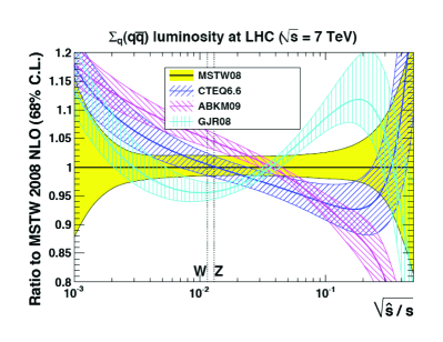
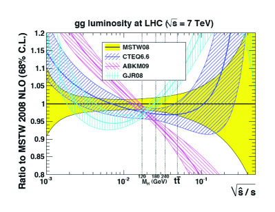
Now we turn to compare the results of the various PDF sets for the LHC observables with the common benchmark settings discussed above. To perform a more meaningful comparison, it is useful to first introduce the idea of differential parton-parton luminosities. Such luminosities, when multiplied by the dimensionless cross section for a given process, provide a useful estimate of the size of an event cross section at the LHC. Below we define the differential parton-parton luminosity :
| (27) |
The prefactor with the Kronecker delta avoids double-counting in case the partons are identical. The generic parton-model formula
| (28) |
can then be written as
| (29) |
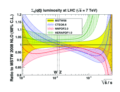
Relative quark-antiquark and gluon-gluon PDF luminosities are shown in Figures 4 and 5. CTEQ6.6, NNPDF2.0, HERAPDF1.0, MSTW08, ABKM09 and GJR08 PDF luminosities are shown, all normalized to the MSTW08 central value, along with their 68 %c.l. error bands. The inner uncertainty bands (dashed lines)for HERAPDF1.0 correspond to the (asymmetric) experimental errors, while the outer uncertainty bands (shaded regions) also includes the model and parameterisation errors. It is interesting to note that the error bands for each of the PDF luminosities are of similar size. The predictions of W/Z, and Higgs cross sections are in reasonable agreement for CTEQ, MSTW and NNPDF, while the agreement with ABKM, HERAPDF and GJR is somewhat worse. (Note however that these plots do not illustrate the effect that the different values used by different groups will have on (mainly) and Higgs cross sections.) It is also notable that the PDF luminosities tend to differ at low and high , for both and luminosities. The CTEQ6.6 distributions, for example, may be larger at low than MSTW2008, due to the positive-definite parameterization of the gluon distribution; the MSTW gluon starts off negative at low and and this results in an impact for both the gluon and sea quark distributions at larger values. The NNPDF2.0 luminosity tends to be somewhat lower, in the region for example. Part of this effect might come from the use of a ZM heavy quark scheme, although other differences might be relevant.

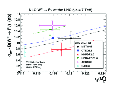
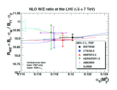
After having performed the comparison between PDF luminosities, we turn to the comparison of LHC observables. Perhaps the most useful manner to perform this comparison is to show the cross–sections as a function of , with an interpolating curve connecting different values of for the same group, when available [27] (see Figs. 6-9). Following the interpolating curve, it is possible to compare cross sections at the same value of . The predictions for the CTEQ, MSTW and NNPDF and cross sections at 7 TeV (Figs. 6-7) agree well, with the NNPDF predictions somewhat lower, consistent with the behaviour of the luminosity observed in Fig. 4. The cross sections from HERAPDF1.0 and ABKM09 are somewhat larger 666Updated versions of these plots, including an extension to NNLO, will be presented in a forthcoming MSTW publication. See also Ref. [1].. The impact from the variation of the value of is relatively small. Basically, all of the PDFs predict similar values for the cross section ratio; much of the remaining uncertainty in this ratio is related to uncertainties in the strange quark distribution. This will serve as a useful benchmark at the LHC. A larger variation in predictions can be observed for the ratio (see Fig. 7). This quantity depends on the separation of the quarks into flavours and the separation between quarks and antiquarks. The data providing this information only extends down to , and consists partially of neutrino DIS off nuclear targets. Hence, different groups provide different results because they fit different choices of data, make different assumptions about nuclear corrections and make different assumptions about the parametric forms of nonsinglet quarks relevant for .


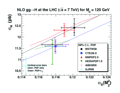
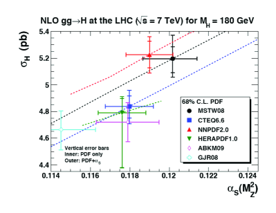
The predictions for Higgs production from fusion (Figs. 8-9) depend strongly on the value of : the anticorrelation between the gluon distribution and the value of is not sufficient to offset the growth of the cross section (which starts at and undergoes a large correction). The CTEQ, MSTW and NNPDF predictions are in moderate agreement but CTEQ lies somewhat lower, to some extent due to the lower choice of . Compared at the common value of , the CTEQ prediction and that of either MSTW or NNPDF, have one-sigma PDF uncertainties which just about overlap for each value of . If the comparison is made at the respective reference values of , but without accounting for the uncertainty, the discrepancies are rather worse, and indeed, even allowing for uncertainty, the bands do not overlap. Hence, both the difference in PDFs and in the dependence of the cross section on the value of are responsible for the differences observed. A useful measure of this is to note that the difference in the central values of the MSTW and CTEQ predictions for a common value of for a 120 GeV Higgs (a typical discrepancy) is equivalent to a change in of about 0.0025. The worst PDF discrepancy is similar to a change of about 0.004. The predictions from HERAPDF are rather lower, reflecting the behaviour of the gluon luminosity of Fig. 5. The ABKM and GJR predictions are also rather lower, but the dependence of results is not explicitly available for these groups, hence it is hard to tell how much of the discrepancy is due to the fact that these groups adopt low values of .
Production of a pair (Fig. 9, right plot) probes the gluon-gluon luminosity at a higher value of , with smaller higher order corrections than present for Higgs production through fusion. The cross section predictions from CTEQ6.6, MSTW2008 and NNPDF2.0 are all seen to be in good agreement, especially when evaluated at the common value of of 0.119.


5.2 Tables of results from each PDF set
In the subsections below, we provide tables of the benchmark cross sections from the PDF groups participating in the benchmark exercise. Only results for 7 TeV will be provided for this interim version of the note.
5.2.1 ABMK09 NLO 5 Flavours
In the following sub-section, the tables of relevant cross sections for the ABKM09 PDFs are given. Results are given for the value of determined from the fit. The charm mass is taken to be GeV and the bottom mass is taken to be GeV. The heavy quark mass uncertainites are incorporated in with the PDF uncertainties.
The results obtained with the ABKM09 NLO 5 flavours set are reported in Tables 1-2.
| Process | Cross section | combined PDF and errors |
|---|---|---|
| 6.3398 | 0.0981 | |
| 4.2540 | 0.0657 | |
| 0.9834 | 0.0151 | |
| 139.55 | 7.96 | |
| 11.663 | 0.314 | |
| 4.718 | 0.147 | |
| 2.481 | 0.092 |
Table 1. Benchmark cross section predictions and uncertainties for ABKM09 NLO for and Higgs production (120, 180, 240 GeV) at 7 TeV. The central prediction is given in column 2. Errors are quoted at the 68% CL. The PDF and errors are evaluated simultaneously. Higgs boson cross sections are corrected for finite top mass effects (1.06, 1.15 and 1.31 for masses of 120, 180 and 240 GeV respectively.
| PDF + Error | PDF + Error | PDF + Error | ||||
|---|---|---|---|---|---|---|
| -4.4 | 0.002 | 0.0005 | 0.0001 | 0.00004 | 0.00002 | 0.000004 |
| -4.0 | 0.102 | 0.0084 | 0.0198 | 0.00262 | 0.00472 | 0.000324 |
| -3.6 | 0.394 | 0.0114 | 0.1228 | 0.01140 | 0.03321 | 0.000909 |
| -3.2 | 0.687 | 0.0324 | 0.2663 | 0.03815 | 0.07542 | 0.002259 |
| -2.8 | 0.878 | 0.0368 | 0.4017 | 0.04089 | 0.10946 | 0.002440 |
| -2.4 | 0.940 | 0.0298 | 0.5328 | 0.01768 | 0.13367 | 0.002566 |
| -2.0 | 0.935 | 0.0180 | 0.6249 | 0.01945 | 0.14787 | 0.002834 |
| -1.6 | 0.915 | 0.0215 | 0.6923 | 0.01479 | 0.15581 | 0.002905 |
| -1.2 | 0.895 | 0.0219 | 0.7344 | 0.01717 | 0.16042 | 0.004083 |
| -0.8 | 0.881 | 0.0241 | 0.7625 | 0.02627 | 0.16298 | 0.003530 |
| -0.4 | 0.867 | 0.0241 | 0.7729 | 0.02364 | 0.16373 | 0.004749 |
| 0.0 | 0.863 | 0.0402 | 0.7774 | 0.02215 | 0.16463 | 0.003186 |
| 0.4 | 0.870 | 0.0411 | 0.7733 | 0.01379 | 0.16352 | 0.005058 |
| 0.8 | 0.871 | 0.0254 | 0.7603 | 0.01647 | 0.16260 | 0.003751 |
| 1.2 | 0.891 | 0.0461 | 0.7348 | 0.02070 | 0.16092 | 0.003715 |
| 1.6 | 0.926 | 0.0589 | 0.6920 | 0.01416 | 0.15539 | 0.004267 |
| 2.0 | 0.934 | 0.0234 | 0.6255 | 0.01680 | 0.14750 | 0.003665 |
| 2.4 | 0.938 | 0.0161 | 0.5279 | 0.01737 | 0.13373 | 0.003013 |
| 2.8 | 0.873 | 0.0244 | 0.4045 | 0.01109 | 0.10944 | 0.002216 |
| 3.2 | 0.692 | 0.0173 | 0.2658 | 0.00600 | 0.07541 | 0.001574 |
| 3.6 | 0.393 | 0.0123 | 0.1254 | 0.00765 | 0.03353 | 0.001316 |
| 4.0 | 0.100 | 0.0057 | 0.0178 | 0.00434 | 0.00441 | 0.000361 |
| 4.4 | 0.002 | 0.0004 | 0.0001 | 0.00003 | 0.00001 | 0.000003 |
Table 2. Benchmark cross section predictions ( in nb) for ABKM09 NLO with for production at 7 TeV, as a function of boson rapidity.
5.2.2 CTEQ6.6
In the following sub-section, the tables of relevant cross sections for the CTEQ6.6 PDFs are given (Tables 3-6). The predictions for the central value of are given in bold. Errors are quoted at the 68% c.l. For CTEQ6.6, this involves dividing the normal 90%c.l. errors by a factor of 1.645.
| )[nb] | |||
| 0.116 | 5.957 | 4.044 | 0.9331 |
| 0.117 | 5.993 | 4.068 | 0.9384 |
| 0.119 | 6.064 | 4.114 | 0.9485 |
| 0.120 | 6.105 | 4.139 | 0.9539 |
Table 3: Benchmark cross section predictions for CTEQ6.6 for and production at 7 TeV, as a function of . The results for the central value of for CTEQ6.6 (0.118) are shown in bold.
| 0.116 | 11.25 | 4.69 | 2.52 | 149.2 |
|---|---|---|---|---|
| 0.117 | 11.42 | 4.76 | 2.57 | 153.0 |
| 0.119 | 11.75 | 4.91 | 2.66 | 160.5 |
| 0.120 | 11.92 | 4.99 | 2.70 | 164.3 |
Table 4: Benchmark cross section predictions for CTEQ6.6 for production (masses of 120, 180 and 240 GeV), and for production, at 7 TeV, as a function of . The results for the central value of for CTEQ6.6 (0.118) are shown in bold. Higgs production ross sections have been corrected for the finite top mass effect (a factor of 1.06 for 120 GeV, 1.15 for 180 GeV and 1.31 for 240 GeV).
| Process | PDF (asym) | PDF (sym) | error | combined | correlation | |
|---|---|---|---|---|---|---|
| 6.057 | +0.123/-0.119 | 0.116 | 0.045 | 0.132 | 0.87 | |
| 4.106 | +0.088/-0.091 | 0.088 | 0.029 | 0.092 | 0.92 | |
| 0.9469 | +0.018/-0.018 | 0.018 | 0.006 | 0.0187 | 1.00 | |
| 156.2 | +7.0/-6.7 | 6.63 | 4.59 | 8.06 | -0.74 | |
| 11.59 | +0.19/-0.23 | 0.21 | 0.20 | 0.29 | 0.01 | |
| 4.840 | +0.077/-0.091 | 0.084 | 0.091 | 0.124 | -0.47 | |
| 2.610 | +0.054/-0.058 | 0.056 | 0.055 | 0.078 | -0.73 |
Table 5: Benchmark cross section predictions and uncertainties for CTEQ6.6 for and Higgs production (120, 180, 240 GeV) at 7 TeV. The central prediction is given in column 2. Errors are quoted at the 68% c.l.. Both the symmetric and asymmetric forms for the PDF errors are given. In the next-to-last column, the (symmetric) form of the PDF and errors are added in quadrature. In the last column, the correlation cosine with respect to production is given.
| PDF Error | PDF Error | PDF Error | ||||
|---|---|---|---|---|---|---|
| -4.4 | 0.002 | 0.0005 | 0.000 | 0.0000 | 0.000 | 0.0000 |
| -4.0 | 0.094 | 0.006 | 0.019 | 0.0063 | 0.005 | 0.00032 |
| -3.6 | 0.367 | 0.013 | 0.122 | 0.0126 | 0.031 | 0.00109 |
| -3.2 | 0.634 | 0.016 | 0.274 | 0.013 | 0.071 | 0.00184 |
| -2.8 | 0.806 | 0.0187 | 0.414 | 0.0128 | 0.106 | 0.00235 |
| -2.4 | 0.878 | 0.019 | 0.517 | 0.0131 | 0.127 | 0.00255 |
| -2.0 | 0.886 | 0.018 | 0.597 | 0.0134 | 0.141 | 0.00255 |
| -1.6 | 0.883 | 0.018 | 0.653 | 0.0144 | 0.148 | 0.00286 |
| -1.2 | 0.867 | 0.020 | 0.697 | 0.017 | 0.155 | 0.00347 |
| -0.8 | 0.862 | 0.023 | 0.723 | 0.02 | 0.166 | 0.00408 |
| -0.4 | 0.855 | 0.025 | 0.739 | 0.023 | 0.161 | 0.00469 |
| 0.0 | 0.864 | 0.026 | 0.750 | 0.0236 | 0.162 | 0.0049 |
| 0.4 | 0.854 | 0.025 | 0.740 | 0.0226 | 0.161 | 0.00479 |
| 0.8 | 0.865 | 0.023 | 0.728 | 0.020 | 0.158 | 0.00418 |
| 1.2 | 0.870 | 0.020 | 0.690 | 0.0167 | 0.155 | 0.00347 |
| 1.6 | 0.882 | 0.018 | 0.654 | 0.0144 | 0.148 | 0.00286 |
| 2.0 | 0.890 | 0.018 | 0.606 | 0.0134 | 0.141 | 0.00265 |
| 2.4 | 0.872 | 0.019 | 0.508 | 0.0128 | 0.114 | 0.0025 |
| 2.8 | 0.806 | 0.019 | 0.416 | 0.0128 | 0.106 | 0.00235 |
| 3.2 | 0.640 | 0.016 | 0.274 | 0.0128 | 0.071 | 0.00184 |
| 3.6 | 0.364 | 0.013 | 0.120 | 0.0127 | 0.031 | 0.00109 |
| 4.0 | 0.095 | 0.006 | 0.023 | 0.0064 | 0.005 | 0.00031 |
| 4.4 | 0.003 | 0.0005 | 0.000 | 0.000 | 0.000 | 0.0000 |
Table 6: Benchmark cross section predictions ( in nb) for CTEQ6.6 for production at 7 TeV, as a function of boson rapidity.
5.2.3 GJR
In the following sub-section, the tables of relevant cross sections for the GJR08 PDFs are given (Tables 7-8). The results are given at the fit value of and the errors correspond to the PDF-only errors at 68% c.l.
| Process | Cross section | PDF Error |
|---|---|---|
| 5.74 | 0.11 | |
| 3.94 | 0.08 | |
| 0.897 | 0.014 | |
| 169 | 6 | |
| 10.72 | 0.35 | |
| 4.66 | 0.14 | |
| 2.62 | 0.09 |
Table 7: Benchmark cross section predictions and uncertainties for GJR08 for and Higgs production (120, 180, 240 GeV) at 7 TeV. The results are given at the fit value of and the errors correspond to the PDF-only errors at 68% c.l. Higgs boson cross sections have been corrected for the finite top mass effect (a factor of 1.06 for 120 GeV, 1.15 for 180 GeV and 1.31 for 240 GeV).
| PDF Error | PDF Error | PDF Error | ||||
|---|---|---|---|---|---|---|
| -4.4 | 0.002 | 0.000 | 0.000 | 0.000 | 0.000 | 0.000 |
| -4.0 | 0.091 | 0.003 | 0.018 | 0.004 | 0.004 | 0.000 |
| -3.6 | 0.368 | 0.011 | 0.122 | 0.013 | 0.031 | 0.001 |
| -3.2 | 0.640 | 0.016 | 0.275 | 0.016 | 0.071 | 0.002 |
| -2.8 | 0.789 | 0.018 | 0.424 | 0.016 | 0.106 | 0.002 |
| -2.4 | 0.848 | 0.018 | 0.525 | 0.016 | 0.126 | 0.002 |
| -2.0 | 0.844 | 0.017 | 0.596 | 0.015 | 0.137 | 0.002 |
| -1.6 | 0.831 | 0.016 | 0.633 | 0.014 | 0.141 | 0.002 |
| -1.2 | 0.803 | 0.015 | 0.654 | 0.013 | 0.144 | 0.002 |
| -0.8 | 0.785 | 0.015 | 0.668 | 0.013 | 0.143 | 0.002 |
| -0.4 | 0.777 | 0.014 | 0.672 | 0.013 | 0.144 | 0.003 |
| 0.0 | 0.780 | 0.014 | 0.677 | 0.013 | 0.145 | 0.003 |
| 0.4 | 0.777 | 0.014 | 0.673 | 0.013 | 0.144 | 0.003 |
| 0.8 | 0.789 | 0.015 | 0.670 | 0.013 | 0.145 | 0.003 |
| 1.2 | 0.806 | 0.015 | 0.655 | 0.013 | 0.143 | 0.002 |
| 1.6 | 0.823 | 0.016 | 0.631 | 0.014 | 0.142 | 0.002 |
| 2.0 | 0.852 | 0.017 | 0.596 | 0.015 | 0.137 | 0.002 |
| 2.4 | 0.842 | 0.018 | 0.527 | 0.016 | 0.126 | 0.002 |
| 2.8 | 0.791 | 0.018 | 0.422 | 0.016 | 0.106 | 0.002 |
| 3.2 | 0.636 | 0.016 | 0.278 | 0.016 | 0.072 | 0.002 |
| 3.6 | 0.371 | 0.011 | 0.117 | 0.013 | 0.031 | 0.001 |
| 4.0 | 0.092 | 0.003 | 0.019 | 0.004 | 0.004 | 0.000 |
| 4.4 | 0.023 | 0.000 | 0.000 | 0.000 | 0.000 | 0.000 |
Table 8: Benchmark cross section predictions ( in nb) for GJR for production at 7 TeV, as a function of boson rapidity. The results are given at the fit value of and the errors correspond to the PDF errors at 68% CL.
5.2.4 HERAPDF1.0
In the following sub-section, the tables of relevant cross sections for the HERAPDF1.0 PDFs are given (Tables 9-10). The predictions for the central value of are given in bold.
| Process | Exp. error | Model error | Param. error | error | Total error | |
|---|---|---|---|---|---|---|
| [nb] | ||||||
| [nb] | ||||||
| [nb] | ||||||
| [pb] | ||||||
| [pb] | ||||||
| [pb] | ||||||
| [pb] |
Table 9: Benchmark cross section predictions and uncertainties for HERAPDF1.0 for and Higgs production (120, 180, 240 GeV) at 7 TeV. The central prediction is given in column 2. Errors are quoted at the 68% c.l. The column labeled Exp. errors stands for the symmetric experimental uncertainty, Model error — for the asymmetric model uncertainty, Param. error — for the asymmetric parameterization uncertainty and error for the uncertainty due to the variation. The Total error stands for the total uncertainty calculated by adding the negative and positive variations in quadrature. Higgs boson cross sections have been corrected for the finite top mass effect (a factor of 1.06 for 120 GeV, 1.15 for 180 GeV and 1.31 for 240 GeV).
| PDF Error | PDF Error | PDF Error | ||||
|---|---|---|---|---|---|---|
Table 10: Benchmark cross section predictions ( in nb) for HERAPDF1.0 set calculated at as a function of boson rapidity. All sources of error calculated above are included.
5.2.5 MSTW2008
In the following sub-section, the tables of relevant cross sections for the MSTW2008 PDFs are given (Tables 11-14). The predictions for the central value of are given in bold.
| )[nb] | |||
| 0.1187 | 5.897 | 4.150 | 0.9336 |
| 0.1194 | 5.927 | 4.171 | 0.9398 |
| 0.1208 | 5.982 | 4.208 | 0.9479 |
| 0.1214 | 6.008 | 4.225 | 0.9516 |
| 0.1190 | 5.911 | 4.160 | 0.9374 |
Table 11: Benchmark cross section predictions for MSTW 2008 for and production at 7 TeV, as a function of . The results for the central value of for MSTW 2008 (0.1202) are shown in bold.
| 0.1187 | 12.13 | 5.08 | 2.74 | 163.5 |
|---|---|---|---|---|
| 0.1194 | 12.27 | 5.14 | 2.77 | 165.8 |
| 0.1208 | 12.53 | 5.24 | 2.83 | 170.0 |
| 0.1214 | 12.64 | 5.29 | 2.86 | 171.9 |
| 0.1190 | 12.18 | 5.10 | 2.76 | 164.4 |
Table 12: Benchmark cross section predictions for MSTW 2008 for production (masses of 120, 180 and 240 GeV), and for production, at 7 TeV, as a function of . The results for the central value of for MSTW 2008 (0.1202) are shown in bold. Cross sections have been corrected for the finite top mass effect (a factor of 1.06 for 120 GeV, 1.15 for 180 GeV and 1.31 for 240 GeV).
| Process | PDF (asym) | PDF (sym) | error | combined | |
|---|---|---|---|---|---|
| 5.957 | +0.129/-0.097 | 0.107 | +0.051/-0.060 | +0.145/-0.121 | |
| 4.190 | +0.092/-0.071 | 0.079 | +0.035/-0.040 | +0.104/-0.080 | |
| 0.944 | +0.020/-0.014 | 0.017 | +0.007/-0.009 | +0.023/-0.0018 | |
| 168.1 | +4.7/-5.6 | 4.9 | +3.8/-4.6 | +7.2/-6.0 | |
| 12.41 | +0.17/-0.21 | 0.19 | +0.23/-0.28 | +0.40/-0.34 | |
| 5.194 | +0.090/-0.106 | 0.095 | +0.094/-0.115 | +0.177/-0.136 | |
| 2.806 | +0.057/-0.069 | 0.062 | +0.052/-0.063 | +0.101/-0.077 |
Table 13: Benchmark cross section predictions and uncertainties for MSTW 2008 for and Higgs production (120, 180, 240 GeV) at 7 TeV. The central prediction is given in column 2. Errors are quoted at the 68% c.l. The symmetric and asymmetric forms for the PDF errors are given. The uncertainty is the deviation of the central prediction at the upper and lower 68% c.l. values of . The combination follows the procedure outlined in the text.
| PDF + Error | PDF + Error | PDF + Error | ||||
|---|---|---|---|---|---|---|
| -4.4 | 0.0024 | 0.0001 | 0.00007 | 0.00003 | 0.000011 | 0.000001 |
| -4.0 | 0.087 | 0.003 | 0.014 | 0.002 | 0.0037 | 0.0001 |
| -3.6 | 0.353 | 0.017 | 0.113 | 0.006 | 0.029 | 0.001 |
| -3.2 | 0.616 | 0.021 | 0.276 | 0.011 | 0.070 | 0.002 |
| -2.8 | 0.787 | 0.022 | 0.422 | 0.015 | 0.105 | 0.003 |
| -2.4 | 0.863 | 0.023 | 0.523 | 0.015 | 0.128 | 0.004 |
| -2.0 | 0.888 | 0.022 | 0.608 | 0.017 | 0.141 | 0.003 |
| -1.6 | 0.879 | 0.020 | 0.678 | 0.017 | 0.151 | 0.004 |
| -1.2 | 0.860 | 0.019 | 0.716 | 0.020 | 0.154 | 0.004 |
| -0.8 | 0.843 | 0.027 | 0.736 | 0.018 | 0.157 | 0.005 |
| -0.4 | 0.856 | 0.023 | 0.770 | 0.019 | 0.161 | 0.005 |
| 0.0 | 0.829 | 0.022 | 0.760 | 0.020 | 0.159 | 0.004 |
| 0.4 | 0.834 | 0.023 | 0.765 | 0.021 | 0.161 | 0.005 |
| 0.8 | 0.855 | 0.022 | 0.742 | 0.019 | 0.157 | 0.004 |
| 1.2 | 0.865 | 0.026 | 0.719 | 0.018 | 0.154 | 0.004 |
| 1.6 | 0.875 | 0.021 | 0.677 | 0.021 | 0.151 | 0.003 |
| 2.0 | 0.890 | 0.026 | 0.608 | 0.018 | 0.142 | 0.004 |
| 2.4 | 0.866 | 0.020 | 0.530 | 0.015 | 0.129 | 0.003 |
| 2.8 | 0.798 | 0.020 | 0.413 | 0.014 | 0.104 | 0.003 |
| 3.2 | 0.611 | 0.019 | 0.280 | 0.012 | 0.070 | 0.002 |
| 3.6 | 0.341 | 0.017 | 0.112 | 0.008 | 0.029 | 0.001 |
| 4.0 | 0.096 | 0.003 | 0.015 | 0.002 | 0.0042 | 0.0002 |
| 4.4 | 0.0022 | 0.0001 | 0.00008 | 0.00003 | 0.000010 | 0.000001 |
Table 14: Benchmark cross section predictions ( in nb) for MSTW 2008 for production at 7 TeV, as a function of boson rapidity.
5.2.6 NNPDF2.0
We show results for the NNPDF2.0 PDF set, with the default NNPDF choice of , as well as for other values of in Table 15 for all the benchmark LHC observables. Note that for each value of we provide the central prediction and the associated PDF uncertainties. For the combined PDF+ uncertainty, we assume the benchmark value of as a 1–sigma uncertainty.
Next in Table 16 we provide for the same observables the benchmark cross section predictions and uncertainties for the NNPDF2.0 set with the combined PDF and strong coupling uncertainties at LHC 7 TeV. In the last column, the PDF and errors are combined using exact error propagation as discussed in Sect. 3.2.4.
Finally in Table 17 we provide the benchmark cross section predictions for the differential rapidity distributions (BR in pb) for NNPDF2.0 for and production at 7 TeV, as a function of the boson rapidity. We provide for each bin in rapidity the combined PDF and uncertainty using exact error propagation.
| =0.115 | nb | nb |
| =0.117 | nb | nb |
| =0.119 | nb | nb |
| =0.121 | nb | nb |
| =0.123 | nb | nb |
| =0.115 | pb | pb |
| =0.117 | pb | pb |
| =0.119 | pb | pb |
| =0.121 | pb | pb |
| =0.123 | pb | pb |
| =0.115 | pb | pb | pb |
| =0.117 | pb | pb | pb |
| =0.119 | pb | pb | pb |
| =0.121 | pb | pb | pb |
| =0.123 | pb | pb | pb |
Table 15: Benchmark cross section predictions for NNPDF2.0 for , , and Higgs production at 7 TeV, as a function of . The results for the central value of for NNPDF2.0 (0.119) are shown in bold. For each value of we provide both the central prediction and the associated 1–sigma PDF uncertainties. The Higgs boson cross sections have been corrected for the finite top mass effect (1.06,1.15,1.31) for the three values of the Higgs boson mass.
| Process | Cross section | PDF errors (1–) | error | PDF+ error |
|---|---|---|---|---|
| [nb] | 5.80 | 0.15 | 0.04 | 0.16 |
| [nb] | 3.97 | 0.09 | 0.04 | 0.10 |
| [nb] | 0.909 | 0.022 | 0.007 | 0.023 |
| [pb] | 169 | 6 | 4 | 7 |
| [pb] | 12.30 | 0.18 | 0.23 | 0.29 |
| [pb] | 5.22 | 0.10 | 0.10 | 0.14 |
| [pb] | 2.84 | 0.066 | 0.052 | 0.092 |
Table 16: Benchmark cross section predictions and uncertainties for NNPDF2.’ for , , and Higgs production (120, 180, 240 GeV) at LHC 7 TeV. The central prediction is given in column 2. We provide PDF uncertainties as 1–sigma uncertainties. In the last column, the PDF and errors are combined using exact error propagation as discussed in Sect. 3.2.4. The Higgs boson cross sections have been corrected for the finite top mass effect (1.06,1.15,1.31) for the three values of the Higgs boson mass.
| BR | PDF+ error | BR | PDF+ error | BR | PDF+ error | |
|---|---|---|---|---|---|---|
| -4.40 | 0.0024 | 0.0003 | 0.0023 | 0.00025 | 0.00001 | 0.00001 |
| -4.00 | 0.090 | 0.0048 | 0.021 | 0.0021 | 0.0039 | 0.00032 |
| -3.60 | 0.352 | 0.020 | 0.122 | 0.007 | 0.030 | 0.002 |
| -3.20 | 0.588 | 0.023 | 0.279 | 0.014 | 0.070 | 0.0037 |
| -2.80 | 0.771 | 0.030 | 0.395 | 0.016 | 0.102 | 0.0042 |
| -2.40 | 0.842 | 0.030 | 0.500 | 0.020 | 0.124 | 0.0043 |
| -2.00 | 0.862 | 0.029 | 0.569 | 0.018 | 0.136 | 0.0053 |
| -1.60 | 0.851 | 0.025 | 0.624 | 0.020 | 0.144 | 0.0038 |
| -1.20 | 0.827 | 0.040 | 0.655 | 0.015 | 0.147 | 0.0039 |
| -0.80 | 0.831 | 0.020 | 0.687 | 0.021 | 0.150 | 0.0045 |
| -0.40 | 0.819 | 0.023 | 0.692 | 0.017 | 0.151 | 0.0034 |
| 0.00 | 0.815 | 0.020 | 0.701 | 0.019 | 0.153 | 0.0049 |
| 0.40 | 0.836 | 0.024 | 0.713 | 0.016 | 0.154 | 0.0031 |
| 0.80 | 0.820 | 0.023 | 0.678 | 0.016 | 0.149 | 0.0046 |
| 1.20 | 0.840 | 0.026 | 0.667 | 0.017 | 0.149 | 0.0044 |
| 1.60 | 0.858 | 0.029 | 0.623 | 0.020 | 0.145 | 0.0039 |
| 2.00 | 0.860 | 0.029 | 0.583 | 0.024 | 0.140 | 0.0051 |
| 2.40 | 0.861 | 0.029 | 0.508 | 0.019 | 0.126 | 0.0046 |
| 2.80 | 0.771 | 0.032 | 0.397 | 0.017 | 0.099 | 0.0047 |
| 3.20 | 0.598 | 0.024 | 0.260 | 0.013 | 0.066 | 0.0037 |
| 3.60 | 0.338 | 0.017 | 0.119 | 0.007 | 0.030 | 0.0025 |
| 4.00 | 0.076 | 0.004 | 0.018 | 0.0023 | 0.0044 | 0.00037 |
| 4.40 | 0.0016 | 0.0007 | 0.0031 | 0.00031 | 0.00001 | 0.00 |
Table 17: Benchmark cross section predictions (BR in nb) for NNPDF2.0 for and production at 7 TeV, as a function of boson rapidity. We provide for each bin in rapidity the combined PDF and uncertainty using exact error propagation.
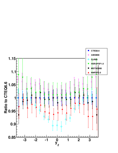
5.3 Comparison of rapidity distributions
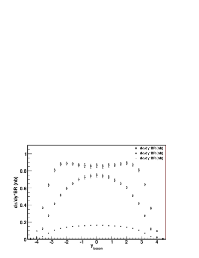
NLO predictions for the and cross sections (along with the PDF uncertainties) are plotted as a function of the boson’s rapidity are plotted in Figure 10 using the CTEQ6.6 PDFs.
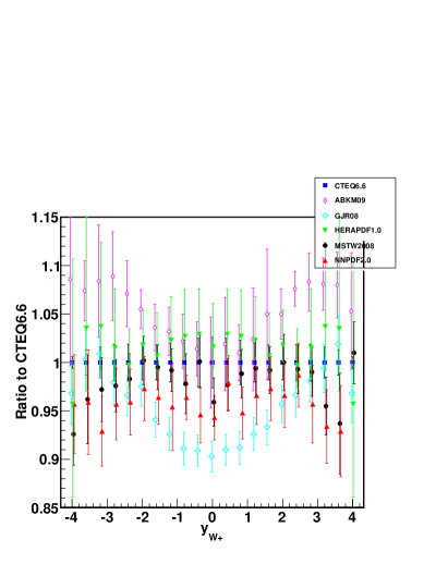
In the figures below, a comparison is made for the predictions of the boson rapidity distributions for the PDFs discussed in this note. In general, the predictions are in reasonable agreement, but differences can be observed that should be detectable with a reasonably-sized data sample at 7 TeV.

6 Summary
In this interim report, we have tried to provide a snapshot of our current understanding of PDFs and the associated experimental and theoretical uncertainties, and of predictions for benchmark cross sections at the LHC (7 TeV) and their corresponding uncertainties. This snapshot will be updated as new input data/theoretical treatments become available. Many of the PDFs discussed in this note are now not the most recent generation from the respective PDF groups, but we have concentrated on these since they are in the most common use by the experimental groups.
References
- [1] S. Alekhin, J. Blümlein,P. Jiminez-Delgado,S. Moch and E. Reya, arXiv:1011.6259 [hep-ph].
- [2] S. Alekhin, J. Blümlein, S. Klein and S. Moch, Phys. Rev. D 81 (2010) 014032 [arXiv:0908.2766 [hep-ph]].
- [3] S. Alekhin, J. Blümlein and S. Moch, PoS D IS2010, 021 (2010) arXiv:1007.3657 [hep-ph].
- [4] P. M. Nadolsky et al., Phys. Rev. D 78 (2008) 013004 [arXiv:0802.0007 [hep-ph]].
- [5] H. L. Lai, M. Guzzi, J. Huston, Z. Li, P. M. Nadolsky, J. Pumplin and C. P. Yuan, Phys. Rev. D82, 074024 (2010). arXiv:1007.2241 [hep-ph].
- [6] M. Glück, P. Jimenez-Delgado and E. Reya, Eur. Phys. J. C 53 (2008) 355 [arXiv:0709.0614 [hep-ph]].
- [7] M. Glück, P. Jimenez-Delgado, E. Reya and C. Schuck, Phys. Lett. B 664, 133 (2008) [arXiv:0801.3618 [hep-ph]].
- [8] F. D. Aaron et al. [H1 Collaboration and ZEUS Collaboration], JHEP 1001 (2010) 109 [arXiv:0911.0884 [hep-ex]].
- [9] A. D. Martin, W. J. Stirling, R. S. Thorne and G. Watt, Eur. Phys. J. C 63 (2009) 189 [arXiv:0901.0002 [hep-ph]].
- [10] R. D. Ball, L. Del Debbio, S. Forte, A. Guffanti, J. I. Latorre, J. Rojo and M. Ubiali, Nucl. Phys. B 838, 136 (2010) [arXiv:1002.4407 [hep-ph]].
- [11] http://indico.cern.ch/conferenceDisplay.py?confId=93790
- [12] D. Stump et al., Phys. Rev. D 65 (2001) 014012 [arXiv:hep-ph/0101051].
- [13] J. Pumplin et al., Phys. Rev. D 65 (2001) 014013 [arXiv:hep-ph/0101032].
- [14] A. D. Martin, R. G. Roberts, W. J. Stirling and R. S. Thorne, Eur. Phys. J. C 28 (2003) 455 [arXiv:hep-ph/0211080].
- [15] R. D. Ball et al. [NNPDF Collaboration], Nucl. Phys. B 809, 1 (2009) [Erratum-ibid. B 816, 293 (2009)] [arXiv:0808.1231 [hep-ph]].
- [16] A. D. Martin, R. G. Roberts, W. J. Stirling and R. S. Thorne, Eur. Phys. J. C 39 (2005) 155 [arXiv:hep-ph/0411040].
- [17] A. D. Martin, W. J. Stirling, R. S. Thorne and G. Watt, Eur. Phys. J. C 70, 51 (2010) [arXiv:1007.2624 [hep-ph]].
- [18] J. Rojo et al., arXiv:1007.0354 [hep-ph].
- [19] F. Demartin, S. Forte, E. Mariani, J. Rojo and A. Vicini, Phys. Rev. D 82 (2010) 014002 [arXiv:1004.0962 [hep-ph]].
- [20] H. L. Lai, J. Huston, Z. Li, P. Nadolsky, J. Pumplin, D. Stump and C. P. Yuan Phys. Rev. D 82, 054021 (2010) arXiv:1004.4624 [hep-ph].
- [21] M. Dittmar et al., arXiv:0901.2504 [hep-ph].
- [22] S. Bethke, Eur. Phys. J. C 64, 689 (2009) [arXiv:0908.1135 [hep-ph]].
- [23] A. D. Martin, W. J. Stirling, R. S. Thorne and G. Watt, Eur. Phys. J. C 64, 653 (2009) [arXiv:0905.3531 [hep-ph]].
- [24] P. M. Nadolsky and Z. Sullivan, in Proc. of the APS/DPF/DPB Summer Study on the Future of Particle Physics (Snowmass 2001) ed. N. Graf, In the Proceedings of APS / DPF / DPB Summer Study on the Future of Particle Physics (Snowmass 2001), Snowmass, Colorado, 30 Jun - 21 Jul 2001, pp P510 [arXiv:hep-ph/0110378].
- [25] http://mcfm.fnal.gov.
- [26] J. Blümlein,S. Riemersma,W. L. van Neerven et al, Nucl.Phys.Proc.Suppl. 51C(1996) 97 [hep-ph/9609217].
- [27] G. Watt, presented at the PDF4LHC meeting of March 26, 2010 (CERN). Plots from http://projects.hepforge.org/mstwpdf/pdf4lhc/ .
- [28] J. R. Andersen et al. [SM and NLO Multileg Working Group], arXiv:1003.1241 [hep-ph].