Ground-state cooling of a suspended nanowire through inelastic macroscopic quantum tunneling in a current-biased Josephson junction

Abstract

We demonstrate that a suspended nanowire forming a weak link between two superconductors can be cooled to its motional ground state by a supercurrent flow. The predicted cooling mechanism has its origins in magnetic field induced inelastic tunneling of the macroscopic superconducting phase associated with the junction. Furthermore, we show the voltage-drop over the junction is proportional to the average population of the vibrational modes in the stationary regime, a phenomena which can be used to probe the level of cooling.

Nanoelectromechanical systems (NEMS) are fast approaching the limits set by quantum mechanics Schwab and Roukes (2005); Blencowe (2005, 2004). Achieving such conditions requires that the mechanical subsystem can be brought into, and detected, in its quantum mechanical ground state. In general this condition demands that an energy quanta associated with the mechanical motion is much larger than the energy associated with the thermal environment. For an oscillator with a mechanical frequency of 100 MHz this implies temperatures as low as a few mK. However, using oscillators with higher mechanical frequencies the quantum limit can be reached, as recently demonstrated by O’Connell et al. O’Connell et al. (2010).

The most common device geometries of NEMS to date consist of mechanical oscillators in the form of cantilevers, suspended beams or microtoroids. These typically have much lower resonance frequencies than those reported in Ref. O’Connell et al. (2010), hence reaching the quantum limit in these devices is very challenging. To circumvent this problem, back-action cooling of the mechanically compliant element is often employed whereby the number of mechanical vibrons is reduced without necessarily lowering the ambient temperature. Suggestions for different cooling mechanisms are plentiful, see e.g. Refs. Martin et al. (2004); Ouyang et al. (2009); Wilson-Rae et al. (2004); Zippilli et al. (2009); Sonne et al. (2010). Common to these is that the oscillator is cooled either by coupling its mechanical oscillations to electromagnetic photons or a flow of charge carriers.

In the present paper we suggest a new mechanism of cooling not previously considered and show that ground-state cooling of the mechanical oscillator is possible. Considering the nanomechanical oscillator as a weak link in a current-biased Josephson junction we show that we can access a regime analogous to the resolved side-band limit Schliesser et al. (2008), whereby the number of mechanical vibrons in the system can be reduced by a factor of $\sim$100 . In the limit of a high mechanical quality factor the resulting vibron population is shown to be well within the quantum regime.

Figure 1: (Color online) Schematic diagram of the system. (Left) A suspended nanowire of length $L$ forms a weak link between two current-biased superconducting leads. The transverse magnetic field $H$ is applied perpendicular to the nanowire. (Right) The equivalent electronic circuit. A constant current $I$ is applied to the Josephson junction which is connected in parallel to a capacitor $C$ and a resistance $R$.

The cooling mechanism considered here is achieved by coupling the mechanical vibrations of the oscillator to the supercurrent through the junction. Below we show that the suggested setup not only allows for ground-state cooling of the mechanical oscillator, but simultaneously probes the macroscopic nature of the superconducting phase associated with the junction. As such, the proposed system allows for interesting physical observations on both the mechanical and the electronic subsystems.

Figure 1 shows a schematic picture of the system considered. It consists of a metallic carbon nanotube suspended over two superconducting leads biased at a current $I$. Transverse to the in-plane motion of the nanotube a magnetic field $H$ is applied which induces coupling between the bending modes of the wire to the supercurrent through it Sonne et al. (2008). Below we analyze the influence of the electromechanical coupling and show that for resonant current-biased conditions this may lead to ground-state cooling of the vibrations of the nanowire.

In our analysis we restrict the description of the mechanical degrees of freedom of the nanowire to the fundamental bending mode, which is considered as a harmonic oscillator with frequency $\omega$. The Hamiltonian describing the system presented in Fig. 1 has the form,

$$\!\!\!\!\hat{\mathcal{H}}=4E_{c}\hat{n}^{2}-j\hbar\hat{\phi}-E_{J}\cos(\hat{\phi}-\Phi\hat{u})+\hbar\omega\hat{b}^{\dagger}\hat{b}\,.$$ (1)

Here, $\hat{n}$ is the operator for the number of Cooper pairs on the junction and $\hat{\phi}$ is the corresponding operator for the superconducting phase Ingold and Nazarov (1992) ($[\hat{\phi},\hat{n}]=i$). In (1), $E_{c}=e^{2}/(2C)$ is the Coulomb energy where $C$ is the capacitance of the junction, $j=I/(2e)$ is the flow of Cooper pairs and $E_{J}$ is the Josephson energy. The operators $\hat{b}^{\dagger}$ $[\hat{b}]$ are creation [annihilation] operators for the oscillator where $\hat{u}=\hat{b}+\hat{b}^{\dagger}$ is the dimensionless deflection of the wire. In the above, the parameter $\Phi=4g\pi LHu_{zp}/\Phi_{0}$ characterizes the strength of coupling between the mechanical and electronic degrees of freedom. Here, $u_{zp}=(\hbar/(2m\omega))^{1/2}$ is the zero-point amplitude of the nanowire, $m$ and $L$ is the effective mass and length of the suspended part of the wire respectively, $\Phi_{0}=\pi\hbar/e$ is the flux quantum and $g$ is a numerical factor of the order of unity which accounts for the profile of the fundamental bending mode Shekhter et al. (2006).

The third term in (1) describes on the one hand the Lorentz force on the nanowire induced by the Josephson current. On the other hand, it gives the deflection-dependence of the Josephson current due to the motion of the wire in the magnetic field Sonne et al. (2008). In what follows we consider a nanotube of length $L\sim 1$$\mu$m, for which $u_{zp}\lesssim 1$ , in a magnetic field $H\sim 1$T. With these parameters $\Phi\lesssim 0.3$, and we consider only the linear terms in the expansion of (1) with respect to $\Phi$. With this expansion the Hamiltonian reads,

$$\hat{\mathcal{H}}=\hat{\mathcal{H}}_{J}+\hat{\mathcal{H}}_{m}+\hat{\mathcal{H}}_{int}\,,$$ (2)

$$\hat{\mathcal{H}}_{J}=4E_{c}\hat{n}^{2}-j\hbar\hat{\phi}-E_{J}\cos\hat{\phi}\,,\qquad\hat{\mathcal{H}}_{m}=\hbar\omega\hat{b}^{\dagger}\hat{b}\,,$$

$$\hat{\mathcal{H}}_{int}=-E_{J}\Phi(\hat{b}^{\dagger}+\hat{b})\sin\hat{\phi}\,.$$

Here, $\hat{\mathcal{H}}_{J}$ is the Josephson Hamiltonian, which under the condition $j<E_{J}/\hbar$, describes the electronic subsystem in the so-called tilted washboard potential. In (2), $\hat{\mathcal{H}}_{int}$ describes the interaction between the mechanical and electronic subsystems with $\hat{\mathcal{H}}_{m}$ the Hamiltonian of the former.

Below we will take the Columb energy to be much smaller than the Josephson energy, $4E_{c}/E_{J}\ll 1$. This condition implies that the characteristic interlevel distance between the quantized states of the Josephson junction associated with a given local minimum of the washboard potential, $\hbar\omega_{p}=(8E_{J}E_{c})^{1/2}$, is much smaller than the height of the barrier separating different local minima. Here, $\omega_{p}$ is the plasma frequency of the junction. We also take the external temperature $T$ to be low, $T<\hbar\omega_{p}/k_{B}$, such that transitions between states associated with different local minima can only occur through under-barrier tunneling. A schematic diagram of the quantum state of the electronic subsystem described through $\hat{\mathcal{H}}_{J}$ is shown in Fig. 2.

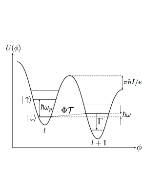
Figure 2: (Color online) Schematic diagram of the tilted washboard potential $U(\phi)=-E_{J}\cos\phi-j\hbar\phi$ as a function of phase $\phi$ at current-bias $I=e/\pi(\omega_{p}-\omega)$. Here, $l$ labels the valleys of the potential and $\sigma=\uparrow,\downarrow$ are the two energy levels within the valleys considered. In the above, $\Phi\mathcal{T}$ is the inelastic tunneling amplitude between two energy levels in consecutive valleys. The quantity $\Gamma$ is the transition rate from the second to the first level within a valley generated by interactions with the quasiparticle environment (see text).

Under-barrier tunneling between two consecutive valleys in Fig. 2 changes the state of the Josephson junction through the associated change of the phase. Such tunneling events, commonly referred to as macroscopic quantum tunneling (MQT), are greatly enhanced if the two energy levels involved in the transition are in resonance. This can be achieved by tuning the current-bias. Thus, we define the critical bias current $I^{*}$ as the current which ensures that the lowest (first) level in a given valley is resonant with the second level in the next valley, $I^{*}\simeq e\omega_{p}/\pi$ Schmidt et al. (1991). As the potential defined by $\hat{\mathcal{H}}_{J}$ is only to first approximation parabolic, the spacing between the energy levels within a given valley is not constant. As such, we will in the following only consider tunneling between the two lowest electronic states and neglect any coupling to higher levels. This is justified as the, e.g., the second and third levels are far from resonance if the junction is biased at $I\simeq I^{*}$ (see Fig. 2) Schmidt et al. (1991).

The electronic system in Fig. 2 is coupled to the mechanical subsystem by the magnetic field. As such, MQT can in the present situation also be accompanied with the emission/absorption of a quanta of mechanical energy, $\hbar\omega$. Performing a WKB analysis for the MQT amplitude we find that the overlap integrals for the inelastic channels is of the order of $\Phi\mathcal{T}$ where $\mathcal{T}\propto\hbar\omega_{p}\exp(-\pi(E_{J}/(2E_{c})^{1/2})<\hbar\omega$ is the tunneling amplitude in the elastic channel. Here, we note that the $\phi$-dependence of $\hat{\mathcal{H}}_{int}$ only leads to a renormalization of the parameter $g$ in the definition of $\Phi$. Also note that due to the large separation in energy, $\omega\ll\omega_{p}$, the electromechanical coupling will not introduce additional tunneling channels between the higher electronic energy levels.

The inelastic tunneling channels change the number of mechanical vibrons such that cooling of the oscillator is possible if transitions through the absorption channel can be promoted. Below we show that this can be achieved by tuning the bias current so that the absorption channel is resonant; the first level in a valley $l$ is separated by $\hbar\omega$ from the second level in $l+1$ as shown in Fig. 2. A further condition for cooling is that the electronic subsystem, once in the second energy level, relaxes to the lower level at a rate $\Gamma$ which is faster than the rate at which the system tunnels back with the emission of a vibron, $\Gamma>\mathcal{T}/\hbar$. Such relaxation arises due to interaction with the quasiparticle environment as discussed further below.

To perform a quantitative analysis of the system we introduce the basis $|l,\sigma\rangle$ where $l$ labels the valleys of the potential and $\sigma=\uparrow,\downarrow$ labels the energy levels inside a given valley ($\downarrow$ is the first and $\uparrow$ is the second level). In this basis the Hamiltonian reads,

$$\hat{\mathcal{H}}=\hat{\mathcal{H}}_{0}+\hat{\mathcal{H}}_{\mathcal{T}}\,,$$ (3)

$$\hat{\mathcal{H}}_{0}=\hat{\mathcal{H}}_{J}+\hat{\mathcal{H}}_{m}=\sum_{l,n,\sigma}(\mathcal{F}_{l,\sigma}+\hbar\omega\hat{b}^{\dagger}\hat{b})|l,\sigma\rangle\langle l,\sigma|\,,$$

$$\hat{\mathcal{H}}_{\mathcal{T}}=\sum_{l}\mathcal{T}\left(\Phi(\hat{b}+\hat{b}^{\dagger})+1\right)|l+1,\uparrow\rangle\langle l,\downarrow|+\textrm{h.c.}\,.$$

In the above, $\mathcal{F}_{l,\sigma}=\hbar\omega_{p}m_{\sigma}-l\pi\hbar I/e$ are the eigenvalues for the electronic degrees of freedom in the basis $|l,\sigma\rangle$, where $m_{\uparrow}=1$ and $m_{\downarrow}=0$. From the form of the Hamiltonian (3) one can see that due to the electromechanical coupling the number of vibrons in the system is not conserved and may change due to macroscopic tunneling of the electronic system from one valley to the next.

To describe the joint dynamics of the electronic and mechanical degrees of freedom we will start our analysis from the Liouville-von Neumann equation for the density matrix $\hat{\rho}$ of the system,

$$\frac{\partial\hat{\rho}}{\partial t}=-\frac{i}{\hbar} \left[\hat{\mathcal{H}}_{0}+\hat{\mathcal{H}}_{\mathcal{T}},\hat{\rho}\right]+\hat{J}(\hat{\rho})+$$

$$\gamma(1+n_{B})\mathcal{L}_{\hat{b}}(\hat{\rho})+\gamma n_{B}\mathcal{L}_{\hat{b}^{\dagger}}(\hat{\rho})\,.$$ (4)

Here, $\hat{J}(\hat{\rho})$ is a phenomenological damping operator for the electronic system Schmidt et al. (1991),

$$\hat{J}(\hat{\rho})=- \frac{\Gamma}{2}\left(\sum_{l}|l,\uparrow\rangle\langle l,\uparrow|\hat{\rho}+\hat{\rho}|l,\uparrow\rangle\langle l,\uparrow|\right)+$$

$$\Gamma \sum_{l,l^{\prime}}|l,\downarrow\rangle\langle l,\uparrow|\hat{\rho}|l^{\prime},\uparrow\rangle\langle l^{\prime},\downarrow|\,.$$ (5)

In the equivalent circuit scheme (see Fig. 1) this damping derives from the parallel resistance $R$, which in the present situation causes the system to decay from the $\uparrow$ state to the $\downarrow$ state in a given valley. In (5), $\Gamma=\omega_{p}/Q_{el}$ is the electronic damping rate, where $Q_{el}=\omega_{p}RC$ is the corresponding quality factor. Here we consider $Q_{el}\gg~{}1$ which implies that the influence from the electronic quasiparticle environment on the tunneling processes is negligible Schmidt et al. (1991); Esteve et al. (1986); Hatakenaka et al. (1990). We will further suppose that the quality factor $Q_{el}$ is so large that broadening of the second energy level, $\Delta\omega_{p}=\omega_{p}/(2Q_{el})$, is small enough for the inelastic resonance transitions to be resolved, $\Delta\omega_{p}<\omega$.

The second damping term in (Ground-state cooling of a suspended nanowire through inelastic macroscopic quantum tunneling in a current-biased Josephson junction), $\mathcal{L}_{\hat{a}}(\hat{\rho})=(2\hat{a}\hat{\rho}\hat{a}^{\dagger}-\hat{a}^{\dagger}\hat{a}\hat{\rho}-\hat{\rho}\hat{a}^{\dagger}\hat{a})/2$, is the standard Lindblad operator which models interactions between the oscillator and the thermal environment. Here, $\gamma=\omega/Q$ is the mechanical damping rate with $Q$ the quality factor and $n_{B}=(\exp(\beta\hbar\omega)-1)^{-1}$, where $\beta=(k_{B}T)^{-1}$, is the average number of vibrons in thermal equilibrium.

Below we investigate the stationary solution to (Ground-state cooling of a suspended nanowire through inelastic macroscopic quantum tunneling in a current-biased Josephson junction). To find this solution we perform a standard perturbative analysis in the small parameters $\mathcal{T}/(\hbar\Gamma),\gamma/\Gamma\propto\epsilon\ll 1$ and look for a solution of the density matrix of the form $\hat{\rho}=\hat{\rho}_{0}+\epsilon\hat{\rho}_{1}+\epsilon^{2}\hat{\rho}_{2}...$ (for a full derivation of the results presented below see Appendix A). Substituting this into (Ground-state cooling of a suspended nanowire through inelastic macroscopic quantum tunneling in a current-biased Josephson junction) one finds that the leading order solution $\hat{\rho}_{0}$ has the form $\hat{\rho}_{0}=\sum_{l,n}|l,\downarrow,n\rangle\rho_{0}(l,\downarrow,n)\langle l,\downarrow,n|$, where the index $n$ labels the Fock state of the oscillator. From (Ground-state cooling of a suspended nanowire through inelastic macroscopic quantum tunneling in a current-biased Josephson junction) we also find the first order correction $\hat{\rho}_{1}=\sum_{l,n,j=-1,0,1}|l+1,\uparrow,n+j\rangle c_{j}(l,n)\langle l,\downarrow,n|+\textrm{h.c.}$ where the sum $\sum_{l}c_{j}(l,n)\equiv C_{j}(n)$ satisfy the following relation,

$$C_{j}(n)=\frac{\mathcal{T}_{j}^{(n)}P(n)}{-\Delta\mathcal{F}_{j}+i\hbar\Gamma/2}\,,\qquad\!\!\!\!\!\!\!\!\!\mathcal{T}_{j}^{(n)}=\left\{\begin{array}[]{l}\mathcal{T}_{+}^{(n)}=\mathcal{T}\Phi\sqrt{n+1}\\ \mathcal{T}_{0}^{(n)}=\mathcal{T}\\ \mathcal{T}_{-}^{(n)}=\mathcal{T}\Phi\sqrt{n}\,.\end{array}\right.$$ (9)

Here, $P(n)=\sum_{l}\rho_{0}(l,\downarrow,n)$ is the population of the vibrational modes of the oscillator. Developing the perturbative expansion one finds that the equation for the second order term, $\hat{\rho}_{2}$, can only be resolved if $P(n)$ satisfy the following equation,

$$(\Gamma_{-}+ \gamma(1+n_{B}))[(n+1)P(n+1)-nP(n)]+$$

$$(\Gamma_{+}+\gamma n_{B})[nP(n-1)-(n+1)P(n)]=0\,.$$ (10)

Here, $\Gamma_{j}$ are the different tunneling rates; $j=-,0,+$ are respectively the absorption, elastic and emission channel,

$$\Gamma_{\pm}=\Gamma\frac{4\Phi^{2}\mathcal{T}^{2}}{4(\Delta\mathcal{F}_{\pm})^{2}+\hbar^{2}\Gamma^{2}}\,,\qquad\Gamma_{0}=\Gamma\frac{4\mathcal{T}^{2}}{4(\Delta\mathcal{F}_{0})^{2}+\hbar^{2}\Gamma^{2}}\,,$$

$$\Delta\mathcal{F}_{0}=\mathcal{F}_{l+1,\uparrow}-\mathcal{F}_{l,\downarrow}\,,\qquad\Delta\mathcal{F}_{\pm}=\mathcal{F}_{0}\pm\hbar\omega\,.$$

Considering the operator for the potential over the Josephson junction $\hat{V}=i[\hat{\mathcal{H}},\hat{\phi}]/(2e)$ (in our representation $\hat{\phi}=2\pi\sum_{l,\sigma}|l,\sigma\rangle l\langle l,\sigma|$) we find,

$$\hat{V}=\frac{\pi}{ie}\sum_{l}\mathcal{T}\left(\Phi(\hat{b}+\hat{b}^{\dagger})+1\right)|l+1,\uparrow\rangle\langle l,\downarrow|+\textrm{h.c.}\,.$$ (11)

This implies that the stationary bias voltage, $V=\textrm{Tr}(\hat{V}\hat{\rho})$, is zero to leading order in $\hat{\rho}$. Thus, the potential drop is given by the first order correction to the density matrix, $V=\textrm{Tr}(\hat{V}\hat{\rho}_{1})$, which implicitly depends on the coefficients $C_{j}(n)$. Solving equation (10) we find that the average number of vibrons, $\langle n\rangle=\sum_{n}nP(n)$, is given by,

$$\langle n\rangle=\frac{n_{B}\gamma+\Gamma_{+}}{\gamma+\Gamma_{-}-\Gamma_{+}}\,,$$ (12)

and that the voltage drop scales with $\langle n\rangle$ as,

$$V=\frac{\pi\hbar}{e}\left(\Gamma_{-}\langle n\rangle+\Gamma_{0}+\Gamma_{+}(\langle n\rangle+1)\right)\,.$$ (13)

Here we note that the potential drop in the stationary regime is primarily determined by the elastic tunneling rate, $\Gamma_{0}$. This is consistent with the physical processes discussed, i.e. in the limit $\gamma,\Gamma_{+}\rightarrow 0$ we get $\langle n\rangle=0$ (complete ground state cooling as no heating channel is open) and $V\propto\Gamma_{0}$ (the system moves down the tilted washboard potential at the rate $\Gamma_{0}$ which conserves the number of vibrons).

In Fig. 3 we plot both the average stationary population of the mechanical subsystem and the corresponding voltage drop as a function of the bias current. As expected, the lowest occupation is achieved when $I=I^{*}-e\omega/\pi$ (see Fig. 2). In this regime, we find that ground state cooling of the mechanical subsystem is possible if the resolved side-band limit, $\omega>\Gamma$, is achieved. Under conditions when the bias current is $I>I^{*}$ the tunneling events discussed above will lead to pumping of the mechanical subsystem, in which case the above analysis does not apply once the limit $\mathcal{T}(\langle n\rangle+1)\sim\hbar\Gamma$ is reached. This regime will be discussed in future work.

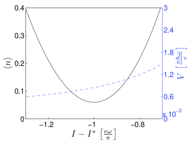
Figure 3: (Color online) Average vibron population (solid) and bias voltage (dashed) in the stationary regime as a function of the current bias. Here, $\Phi=0.3$, $\Gamma=\omega/4$, $\mathcal{T}=\hbar\omega/20$, $n_{B}=20$ and $Q=$$10^{5}$ .

To conclude we have shown that a suspended nanowire which forms a weak link in current-biased Josephson junction can be cooled to its motional ground state. This effect derives from the coupling of the mechanical motion of the nanowire to the electronic degrees of freedom by a magnetic field. Furthermore, we have shown that by operating the system under optimal bias-current conditions the occupation factor of the vibrational modes can be greatly decreased. Also, we have found that the potential drop over the junction might be a sensitive probe of the stationary vibron population as it scales with the average number of vibrons.

This work was supported in part by the Swedish VR and SSF and by the EC project QNEMS (FP7-ICT-233952).

Appendix A Derivation of density matrix

The evolution of the density matrix is governed by the Liouville-von Neumann equation (Ground-state cooling of a suspended nanowire through inelastic macroscopic quantum tunneling in a current-biased Josephson junction),

$$\frac{\partial\hat{\rho}}{\partial t}= -\frac{i}{\hbar}\left[\hat{\mathcal{H}}_{0}+\hat{\mathcal{H}}_{\mathcal{T}},\hat{\rho}\right]+\hat{J}(\hat{\rho})+$$

$$\gamma(1+n_{B})\mathcal{L}_{\hat{b}}(\hat{\rho})+\gamma n_{B}\mathcal{L}_{\hat{b}^{\dagger}}(\hat{\rho})\,.$$ (14)

In what follows we will consider the stationary solution of (A) by performing a perturbative analysis in the small parameters $\mathcal{T}/(\hbar\Gamma),\gamma/\Gamma\ll 1$. In particular we will consider the limit of high mechanical quality factor $Q$ such that $\gamma=\omega/Q<\mathcal{T}/(\hbar)$. To start the analysis we take the total density matrix to be of the form, $\hat{\rho}=\hat{\rho}_{0}+\epsilon\hat{\rho}_{1}+\epsilon^{2}\hat{\rho}_{2}...$ and equate powers of $\epsilon$. With this we find the following equations,

$$0=-\frac{i}{\hbar}\left[\hat{\mathcal{H}}_{0},\hat{\rho}_{0}\right]+\hat{J}(\hat{\rho}_{0})\,,\qquad\qquad\qquad\,\,\,\,\,\,\,\,\,O(\epsilon^{0})\\$$ (15)

$$0=-\frac{i}{\hbar}\left[\hat{\mathcal{H}}_{0},\hat{\rho}_{1}\right]+\hat{J}(\hat{\rho}_{1})-\frac{i}{\hbar}\left[\hat{\mathcal{H}}_{\mathcal{T}},\hat{\rho}_{0}\right]\,,\,\,\,\,\,\,\,O(\epsilon^{1})$$ (16)

$$0= -\frac{i}{\hbar}\left[\hat{\mathcal{H}}_{0},\hat{\rho}_{2}\right]+\hat{J}(\hat{\rho}_{2})-\frac{i}{\hbar}\left[\hat{\mathcal{H}}_{\mathcal{T}},\hat{\rho}_{1}\right]+$$

$$\gamma(1+n_{B})\mathcal{L}_{\hat{b}}(\hat{\rho}_{0})+\gamma n_{B}\mathcal{L}_{\hat{b}^{\dagger}}(\hat{\rho}_{0})\,.\, O(\epsilon^{2})$$ (17)

Solving the above equations at each order of $\epsilon$ we find $\hat{\rho}_{0}=\sum_{l,n}|l,\downarrow,n\rangle\rho_{0}(l,\downarrow,n)\langle l,\downarrow,n|$ which satisfies (15). Similarly, the first order correction to the stationary density matrix is determined from (16) as,

$$\hat{\rho}_{1}=\sum_{\begin{subarray}{c}l,n\\ j=-1,0,1\end{subarray}}|l+1,\uparrow,n+i\rangle c_{j}(l,n)\langle l,\downarrow,n|+\textrm{h.c.}\,,$$

$$c_{j}(l,n)=\frac{\mathcal{T}_{j}^{(n)}\rho_{0}(l,\downarrow,n)}{-\Delta\mathcal{F}_{j}+i\hbar\Gamma/2}\,,$$ (18)

Substituting this into (17) we find the equation for the coefficients $\rho_{0}$ by tracing out the spin ($\uparrow,\downarrow$) degrees of freedom,

$$\Gamma\sum_{j=-1,0,1}\frac{4}{4(\Delta\mathcal{F}_{j})^{2}+\hbar^{2}\Gamma^{2}} \bigg{(}|\mathcal{T}_{j}^{(n-j)}|^{2}\rho_{0}(l-1,\downarrow,n-j)-$$

$$\qquad|\mathcal{T}_{j}^{(n)}|^{2}\rho_{0}(l,\downarrow,n)\bigg{)}=$$

$$\gamma(1+n_{B})[n\rho_{0}(l,\downarrow,n) -(n+1)\rho_{0}(l,\downarrow,n+1)]+$$

$$\gamma n_{B}[(n+1)\rho_{0}(l,\downarrow,n) -n\rho_{0}(l,\downarrow,n-1)]\,.$$ (19)

Tracing out the valley index $l$ we recover the expressions presented in the paper, i.e. equation (18) gives

$$C_{j}(n)\equiv\sum_{l=-\infty}^{\infty}c_{j}(l,n)=\frac{\mathcal{T}_{j}^{(n)}P(n)}{-\Delta\mathcal{F}_{j}+i\hbar\Gamma/2}\,,$$

whereas equation (19) gives,

$$(\Gamma_{-}+ \gamma(1+n_{B}))[(n+1)P(n+1)-nP(n)]+$$

$$(\Gamma_{+}+\gamma n_{B})[nP(n-1)-(n+1)P(n)]=0\,.$$ (20)

In this expression the relationship between the coefficients are,

$$\Gamma_{\pm}=\Gamma\frac{4\Phi^{2}\mathcal{T}^{2}}{4(\Delta\mathcal{F}_{\pm})^{2}+\hbar^{2}\Gamma^{2}}\,,\qquad\Gamma_{0}=\Gamma\frac{4\mathcal{T}^{2}}{4(\Delta\mathcal{F}_{0})^{2}+\hbar^{2}\Gamma^{2}}\,,$$

$$\frac{i}{\hbar}\mathcal{T}_{j}^{(n)}\left(C_{j}(n)-C_{j}^{*}(n)\right)=P(n)\Gamma_{j}N\,,$$

$$N=\left\{\begin{array}[]{lcl}n+1&&j=+\\ 1&&j=0\\ n&&j=-\,.\end{array}\right.$$ (24)

In the above we note that (A) gives the balanced equation for the probability $P(n)$ of finding the oscillating nanowire in the state $n$. The stationary average distribution of the vibrational modes is then given by the solution to this equation,

$$\langle n\rangle=\sum_{n=0}^{\infty}nP(n)=\frac{n_{B}\gamma+\Gamma_{+}}{\Gamma_{-}+\gamma-\Gamma_{+}}\,.$$

The density matrix $\hat{\rho}_{1}$ allow us to evaluate the potential drop over the junction in the stationary regime. Following the derivation outlined in the paper we find that the lowest order term of the density matrix, $\hat{\rho}_{0}$, does not contribute to the potential drop as it is diagonal in the spin basis. As such, the potential drop is uniquely determined from $\hat{\rho}_{1}$.

References

- Schwab and Roukes (2005) K. C. Schwab and M. L. Roukes, Phys. Today, 58, 36 (2005).
- Blencowe (2005) M. P. Blencowe, Contemp. Phys., 46, 249 (2005).
- Blencowe (2004) M. Blencowe, Phys. Rep., 395, 159 (2004).
- O’Connell et al. (2010) A. D. O’Connell, M. Hofheinz, M. Ansmann, R. C. Bialczak, M. Lenander, E. Lucero, M. Neeley, D. Sank, H. Wang, M. Weides, J. Wenner, J. M. Martinis, and A. N. Cleland, Nature, 464, 697 (2010).
- Martin et al. (2004) I. Martin, A. Shnirman, L. Tian, and P. Zoller, Phys. Rev. B, 69, 125339 (2004).
- Ouyang et al. (2009) S. H. Ouyang, J. Q. You, and F. Nori, Phys. Rev. B, 79, 075304 (2009).
- Wilson-Rae et al. (2004) I. Wilson-Rae, P. Zoller, and A. Imamoḡlu, Phys. Rev. Lett., 92, 075507 (2004).
- Zippilli et al. (2009) S. Zippilli, G. Morigi, and A. Bachtold, Phys. Rev. Lett., 102, 096804 (2009).
- Sonne et al. (2010) G. Sonne, M. E. Peña-Aza, L. Y. Gorelik, R. I. Shekhter, and M. Jonson, Phys. Rev. Lett., 104, 226802 (2010).
- Schliesser et al. (2008) A. Schliesser, R. Riviere, G. Anetsberger, O. Arcizet, and T. J. Kippenberg, Nat. Phys., 4, 415 (2008).
- Sonne et al. (2008) G. Sonne, R. I. Shekhter, L. Y. Gorelik, S. I. Kulinich, and M. Jonson, Phys. Rev. B, 78, 144501 (2008).
- Ingold and Nazarov (1992) G.-L. Ingold and Y. V. Nazarov, “Single charge tunneling,” (Plenum Press, New York, 1992) p. 21.
- Shekhter et al. (2006) R. I. Shekhter, L. Y. Gorelik, L. I. Glazman, and M. Jonson, Phys. Rev. Lett., 97, 156801 (2006).
- Schmidt et al. (1991) J. M. Schmidt, A. N. Cleland, and J. Clarke, Phys. Rev. B, 43, 229 (1991).
- Esteve et al. (1986) D. Esteve, M. H. Devoret, and J. M. Martinis, Phys. Rev. B, 34, 158 (1986).
- Hatakenaka et al. (1990) N. Hatakenaka, H. Takayanagi, and S. Kurihara, Physica B, 165-166, 931 (1990).