Critical properties of the two-dimensional Z(5) vector model

Abstract:

The two-dimensional Z(5) vector model is investigated through the determination of critical points and one critical index. To this purpose a new cluster algorithm has been developed valid for $2D$ Z($N$) models with odd values of $N$. Results are compared with analytical predictions.

1 Introduction

The Berezinskii-Kosterlitz-Thouless (BKT) phase transition is known to take place in a variety of two-dimensional ($2D$) systems, the most common being the $2D$ $XY$ model [1]. Here we are going to study an example of lattice spin model where this type of the transition shows up, namely the $2D$ Z($N$) spin model, also known as vector Potts model. On a $2D$ lattice $\Lambda=L^{2}$ with linear extension $L$ and periodic boundary conditions, the partition function of the model can be written as

$$Z(\Lambda,\beta)=\left[\prod_{x\in\Lambda}\frac{1}{N}\sum_{s(x)=0}^{N-1}\right]\left[\prod_{x\in\Lambda}\prod_{n=1,2}Q\left(s(x)-s(x+e_{n})\right)\right]\;,\;\;\;\;\;Q(s)\ =\ \exp\left[\sum_{k=1}^{N-1}\beta_{k}\cos\frac{2\pi k}{N}s\right]\,,$$ (1)

in the standard formulation with $N-1$ different couplings.

Some details of the critical behavior of $2D$ Z($N$) spin models are well known – see the review in Ref. [2]. The Z($N$) spin model in the Villain formulation has been studied analytically in Refs. [3]. It was shown that the model has at least two phase transitions when $N\geq 5$. The intermediate phase is a massless phase with power-like decay of the correlation function. The critical index $\eta$ has been estimated both from the renormalization group (RG) approach of the Kosterlitz-Thouless type and from the weak-coupling series for susceptibility. It turns out that $\eta(\beta^{(1)}_{\rm c})=1/4$ at the transition point from the strong coupling (high-temperature) phase to the massless phase, i.e. the behavior is similar to that of the $XY$ model. At the transition point $\beta^{(2)}_{\rm c}$ from the massless phase to the ordered low-temperature phase one has $\eta(\beta^{(2)}_{\rm c})=4/N^{2}$. A rigorous proof that the BKT phase transition does take place, and so that the massless phase exists, has been constructed in Ref. [4] for both Villain and standard formulations (with one non-vanishing coupling $\beta_{1}$). Monte-Carlo simulations of the standard version with $N=6,8,12$ were performed in Ref. [5]. Results for the critical index $\eta$ agree well with the analytical predictions obtained from the Villain formulation of the model.

Here we investigate the case $N=5$, the lowest number where the BKT transition is expected. The motivation of our study is two-fold: (i) to compute critical indices at the transition points, which could serve as checking point of universality; (ii) to develop and test a Monte Carlo cluster algorithm valid for odd values of $N$, not yet available in the literature, to our knowledge.

2 Algorithm and numerical set-up

In this work we concentrate our attention to the model defined by Eq. (1) with only one non-zero coupling, $\beta_{1}\equiv\beta$. The Hamiltonian of the model is

$$H=-\beta\sum_{\langle ij\rangle}\cos\left(\frac{2\pi}{N}(s_{i}-s_{j})\right)\;,\;\;\;\;\;s_{i}=0,1,\ldots,N-1\;,$$ (2)

with summation taken over nearest-neighbor sites. For $N=2$ this is the Ising model, whereas in the $N\rightarrow\infty$ limit we get the $XY$ model.

A cluster algorithm for the Monte Carlo numerical simulation of this model is available in the literature only for even $N$ [5]. Here we develop a new algorithm, valid instead for odd $N$, by which an accurate numerical study of the model can be performed for $N=5$, i.e. the smallest $N$ value for which the phase structure described in the Introduction holds. Here are the steps of our cluster algorithm for the update of a spin configuration $\{s_{i}\}$:

• choose randomly $n$ in the set $\{0,1,2,\ldots,N-1\}$

• build a cluster configuration according to the following probability of bond activation between neighboring sites $ij$

  $$p_{ij}=\left\{\begin{array}[]{cl}1-\exp(-2\beta\ \alpha_{i}\alpha_{j})&{\rm if}\;\alpha_{i}\alpha_{j}>0\\ 0&{\rm otherwise}\\ \end{array}\right.\;,\;\;\;\;{\rm with}\;\;\alpha_{k}\equiv\sin\left(\frac{2\pi}{N}(s_{k}-n)\right)$$

• “flip” each cluster, with probability 1/2, by replacing all spins belonging to it according to the transformation

  $$s_{i}\rightarrow{\rm mod}(-s_{i}+2n+N,N)\;,$$

  which amounts to replacing each spin $s_{i}$ in a cluster by the spin $s_{j}$ for which $\alpha_{j}=-\alpha_{i}$.

It is easy to prove that this cluster algorithm fulfills the detailed balance. We have tested the efficiency of the cluster algorithm against the standard heat-bath algorithm and found that the cluster algorithm is strongly preferable (see Ref. [6] for details).

Figure 1: Scatter plot of the complex magnetization $M_{L}$ at $\beta=0.80,1.10,1.50$ in $Z(5)$ on a $64^{2}$ lattice.

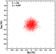
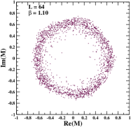
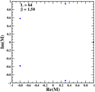
The three phases exhibited by the $2D$ Z(5) spin model can be characterized by means of two observables: the complex magnetization $M_{L}$ and the population $S_{L}$. The complex magnetization is given by

$$M_{L}=\frac{1}{L^{2}}\sum_{i}\exp\left(i\frac{2\pi}{N}s_{i}\right)\equiv|M_{L}|e^{i\psi}\;.$$ (3)

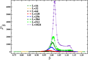
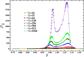
In Fig. 1 we show the scatter plot of $M_{L}$ on a lattice with $L=64$ in $Z(5)$ at three values of $\beta$, each representative of a different phase: $\beta=0.80$ (high-temperature, disordered phase), $\beta=1.10$ (BKT massless phase) and $\beta=1.50$ (low-temperature, ordered phase). As we can see we pass from a uniform distribution (low $\beta$) to a ring distribution (intermediate $\beta$) and finally to five isolated spots (high $\beta$). The naive average of the complex magnetization gives constantly zero, therefore $M_{L}$ is not an order parameter. A convenient observable to detect the transition from one phase to the other is instead the absolute value $|M_{L}|$ of the complex magnetization. In Fig. 2 (left) we show the behavior of the susceptibility of $|M_{L}|$,

$$\chi^{(M)}_{L}=L^{2}(\langle|M_{L}|^{2}\rangle-\langle|M_{L}|\rangle^{2})\;,$$ (4)

in $Z(5)$ on lattices with $L$ ranging from 16 to 1024 over a wide interval of $\beta$ values. On each lattice $\chi^{(M)}_{L}$ clearly exhibits two peaks, the first of them, more pronounced than the other, identifies the pseudo-critical coupling $\beta^{(1)}_{\rm pc}(L)$ at which the transition from the disordered to the massless phase occurs, whereas the second corresponds to the pseudo-critical coupling $\beta^{(2)}_{\rm pc}(L)$ of the transition from the massless to the ordered phase. It is evident from Fig. 2 that $|M_{L}|$ is particularly sensitive to the first transition, thus making this observable the best candidate for studying its properties.

As a local order parameter to better detect the second transition, i.e. that from the massless to the ordered phase, we chose instead the population $S_{L}$, defined as

$$S_{L}=\frac{N}{N-1}\left[\frac{\max_{i=0,N-1}(n_{i})}{L^{2}}-\frac{1}{N}\right]\;,$$ (5)

where $n_{i}$ represents the number of spins of a given configuration which are in the state $s_{i}$. In a phase in which there is not a preferred spin direction in the system (disorder), we have $n_{i}\sim L^{2}/N$ for each index $i$, therefore $S_{L}\sim 0$. Otherwise, in a phase in which there is a preferred spin direction (order), we have $n_{i}\sim L^{2}$ for a given index $i$, therefore $S_{L}\sim 1$. In Fig. 2 (right) we show the behavior of the susceptibility of $S_{L}$,

$$\chi^{(S)}_{L}=L^{2}(\langle S_{L}^{2}\rangle-\langle S_{L}\rangle^{2})\;,$$ (6)

in $Z(5)$ on lattices with $L$ ranging from 16 to 1024 over a wide interval of $\beta$ values. Again the peaks signalling the two transitions are clearly visible and their positions agree with Fig. 2, but now the second one is more pronounced.

Other observables which have been used in this work are the following:

• the real part of the “rotated” magnetization, $M_{R}=|M_{L}|\cos(5\psi)$

• the order parameter introduced in Ref. [7], $m_{\psi}=\cos(5\psi)$,

where $\psi$ is the phase of the complex magnetization defined in Eq. (3). For all observables considered in this work we collected typically 100k measurements, on configurations separated by 10 updating sweeps. For each new run the first 10k configurations were discarded to ensure thermalization. Data analysis was performed by the jackknife method over bins at different blocking levels.

Figure 2: Behavior of the susceptibilities $\chi^{(M)}_{L}$ (left) and $\chi^{(S)}_{L}$ (right) versus $\beta$ in $Z(5)$ on lattices with several values of $L$.

3 Numerical results

The first peak in the plot of the susceptibility $\chi_{L}^{(M)}$ (see Fig. 2 (left)) indicates the transition from the disordered to the massless phase, while the second peak in the plot of the susceptibility $\chi_{L}^{(S)}$ (see Fig. 2(right)) indicates the transition from the massless to the ordered phase. The couplings where these transitions occur (from now on denoted as the pseudo-critical couplings $\beta_{\rm pc}^{(1,2)}(L)$) have been determined by a Lorentzian interpolation around the peak of the corresponding susceptibility. Their values are summarized in Table 1.

Table 1: Values of $\beta^{(1)}_{\rm pc}$ and $\beta^{(2)}_{\rm pc}$ in $Z(5)$ on $L^{2}$ lattices.

$L$	$\beta^{(1)}_{\rm pc}$	$\beta^{(2)}_{\rm pc}$
16	0.8523(20)	1.1323(19)
32	0.91429(90)	1.1363(11)
64	0.95373(40)	1.13212(60)
128	0.98054(30)	1.12875(66)
256	0.99838(20)	1.12290(16)
384	1.00621(10)	1.12103(50)
512	1.01112(20)	1.11912(28)
1024	1.01991(10)	1.11596(38)

In order to apply the finite size scaling (FSS) program, the location of the infinite volume critical couplings $\beta^{(1)}_{\rm c}$ and $\beta^{(2)}_{\rm c}$ is needed. In Refs. [8, 9] this was done by extrapolating the pseudo-critical couplings to the infinite volume limit, according to a suitable scaling law. First order transitions are ruled out by data in Table 1. Second order transitions, though not incompatible with data in Table 1, are to be excluded, due to the vanishing of the long distance correlations combined with the clusterization property. Therefore, we assume that both transitions are of BKT type and adopt the scaling law dictated by the essential scaling of the BKT transition, i.e. $\xi\sim e^{bt^{-\nu}}$, which reads

$$\beta^{(1,2)}_{\rm pc}=\beta^{(1,2)}_{\rm c}+\frac{A_{1,2}}{(\ln L+B_{1,2})^{\frac{1}{\nu}}}\quad.$$ (7)

The index $\nu$ characterizes the universality class of the system. For example, $\nu=1/2$ holds for the 2$D$ $XY$ universality class.

Unfortunately, 4-parameter fits of the data for $\beta^{(1,2)}_{\rm pc}(L)$ give very unstable results for the parameters. This led us to move to 3-parameter fits of the data, with $\nu$ fixed at 1/2. We found, as best fits with the MINUIT optimization code,

$$\begin{array}[]{lllll}\beta^{(1)}_{\rm c}=1.0602(20)&\;\;\;A_{1}=-2.09(20)&\;\;\;B_{1}=0.27(18)&\;\;\;\chi^{2}/{\rm d.o.f.}=0.48&\;\;\;L_{\rm min}=64\\ \beta^{(2)}_{\rm c}=1.1042(12)&\;\;\;A_{2}=0.578(41)&\;\;\;B_{2}=0.&\;\;\;\chi^{2}/{\rm d.o.f.}=0.61&\;\;\;L_{\rm min}=128\end{array}$$

for the first and second transition, respectively. We observe that $\beta^{(2)}_{\rm c}$ is not far from the value of $\beta^{(2)}_{\rm pc}$ on the largest available lattice, thus supporting the reliability of the extrapolation to the thermodynamic limit. This is not the case for $\beta^{(1)}_{\rm c}$, suggesting that the considered volumes could not be large enough for using the scaling law (7). For this reason, we turned to an independent method for the determination of $\beta^{(1,2)}_{\rm c}$, based on the use of Binder cumulants.

In particular, for the study of the first transition, we considered the reduced 4-th order Binder cumulant $U^{(M)}_{L}$ defined as

$$U^{(M)}_{L}=1-\frac{\langle|M_{L}|^{4}\rangle}{3\langle|M_{L}|^{2}\rangle^{2}}\;,$$ (8)

and the cumulant $B_{4}^{(M_{R})}$ defined as

$$B_{4}^{(M_{R})}=\frac{\langle|M_{R}-\langle M_{R}\rangle|^{4}\rangle}{\langle|M_{R}-\langle M_{R}\rangle|^{2}\rangle^{2}}\;,$$ (9)

while for the second transition we adopted again $B_{4}^{(M_{R})}$ and the cumulant $B_{4}^{(m_{\psi})}$ defined as

$$B_{4}^{(m_{\psi})}=\frac{\langle(m_{\psi}-\langle m_{\psi}\rangle)^{4}\rangle}{\langle(m_{\psi}-\langle m_{\psi}\rangle)^{2}\rangle^{2}}\;.$$ (10)

Plots of the various Binder cumulants versus $\beta$ show that data obtained on different lattice volumes align on curves that cross in two points, corresponding to the two transitions. We determined the crossing points by two methods: (i) by interpolating with polynomial lines data on different lattices near the crossing points and by looking for the intersection of these lines; (ii) by plotting the Binder cumulants versus $(\beta-\beta_{\rm c})(\log L)^{1/\nu}$, with $\nu$ fixed at 1/2, and by looking for the optimal overlap of data from different lattices, by the $\chi^{2}$ method. As a result of this analysis (for details, see Ref. [6]) we arrived at the following estimates: $\beta^{(1)}_{\rm c}=1.0510(10)$ and $\beta^{(2)}_{\rm c}=1.1048(10)$. While $\beta^{(2)}_{\rm c}$ is compatible with the infinite volume extrapolation of the corresponding pseudocritical couplings, $\beta^{(1)}_{\rm c}$ is not, thus confirming the previous worries about the safety of the infinite volume extrapolation of $\beta^{(1)}_{\rm pc}$. It should be noted, however, that a fit to $\beta^{(1)}_{\rm pc}(L)$ with the law (7) and with the parameter $\beta^{(1)}_{\rm c}$ fixed at 1.0510 gives a good $\chi^{2}$/d.o.f., if only the three largest volumes are considered in the fit.

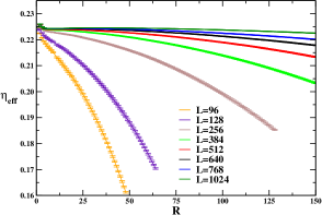
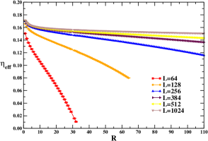
The next step would be to extract other critical indices and check the hyperscaling relations at the two transitions. This calls for the FSS of magnetizations and susceptibilities at the critical couplings $\beta^{(1,2)}_{\rm c}$, which is in progress [6]. We present here only two determinations of the effective $\eta$ index, defined in Ref. [8] as

$$\eta_{\rm eff}(R)\equiv\frac{\log[\Gamma(R)/\Gamma(R_{0})]}{\log[R_{0}/R]}\quad,$$ (11)

where $\Gamma(R)$ is the spin-spin correlation function and $R_{0}$ an arbitrary parameter, chosen here equal to 10. This quantity is constructed in such a way that it exhibits a plateau in $R$ if the correlator obeys the law

$$\Gamma(R)\ \asymp\ \frac{1}{R^{\eta(T)}}\ ,$$ (12)

valid in the BKT phase, $\beta^{(1)}_{\rm c}\leq\beta\leq\beta^{(2)}_{\rm c}$. In Figs. 3 we show the behavior of $\eta_{\rm eff}(R)$ at $\beta=1.0602$, which is slightly above the estimated value for $\beta^{(1)}_{\rm c}$, and at $\beta=1.1083$, which is slightly above the estimated value for $\beta^{(2)}_{\rm c}$. A plateau is visible at small distances when $L$ increases and the extension of this plateau gets larger with $L$, consistently with the fact that finite volume effects are becoming less important. The plateau value of $\eta_{\rm eff}$ is about 0.225 at $\beta$=1.0602, i.e. near the first transition, and about 0.16 near the second transition. These values are not far from the expected ones (1/4 and $4/5^{2}$, respectively). The determination of $\eta_{\rm eff}$ at $\beta^{(1)}_{\rm c}$ and $\beta^{(2)}_{\rm c}$ is in progress [6].

Figure 3: $\eta_{\rm eff}$ versus $R$ at $\beta=1.0602$ (left) on lattices with $L=96,128,256,384,512,640,768,1024$ and at $\beta=1.1083$ (right) on lattices with $L=64,128,256,384,512,1024$.

In conclusion, we have determined the critical couplings of the $2D$ Z(5) vector model and given a rough estimate of the critical index $\eta$ near the transitions. Our findings support the standard scenario of three phases: disordered, massless or BKT and ordered. In a recent work [10] it is claimed that the phase transition at $\beta^{(1)}_{\rm c}$ is not a standard BKT phase transition. We will comment on this point in Ref. [6].

References

- [1] V. Berezinskii, Sov. Phys. JETP 32 (1971) 493; J. Kosterlitz, D. Thouless, J. Phys. C6 (1973) 1181; J. Kosterlitz, J. Phys. C7 (1974) 1046.
- [2] F.Y. Wu, Rev. Mod. Phys. 54 (1982) 235.
- [3] S. Elitzur, R.B. Pearson, J. Shigemitsu, Phys. Rev. D19 (1979) 3698; M.B. Einhorn, R. Savit, A physical picture for the phase transitions in -symmetric models, Preprint UM HE 79-25; C.J. Hamer, J.B. Kogut, Phys. Rev. B22 (1980) 3378; B. Nienhuis, J. Statist. Phys. 34 (1984) 731; L.P. Kadanoff, J. Phys. A11 (1978) 1399.
- [4] J. Fröhlich, T. Spencer, Commun. Math. Phys. 81 (1981) 527.
- [5] Y. Tomita, Y. Okabe, Phys. Rev. B65 (2002) 184405.
- [6] O. Borisenko, G. Cortese, R. Fiore, M. Gravina, A. Papa, in preparation.
- [7] S.K. Baek, P. Minnhagen and B.J. Kim, Phys. Rev. E80 (2009) 060101(R) (2009).
- [8] O. Borisenko, M. Gravina, A. Papa, J. Stat. Mech. 2008 (2008) P08009 [arXiv:0806.2081].
- [9] O. Borisenko, R. Fiore, M. Gravina, A. Papa, J. Stat. Mech. 2010 (2010) P04015 [arXiv:1001.4979].
- [10] S.K. Baek and P. Minnhagen, Phys. Rev. E82 (2010) 031102.